On Euler’s equation and ‘EPDiff’

Abstract.

We study a family of approximations to Euler’s equation depending on two parameters $\varepsilon,\eta\geq 0$. When $\varepsilon=\eta=0$ we have Euler’s equation and when both are positive we have instances of the class of integro-differential equations called EPDiff in imaging science. These are all geodesic equations on either the full diffeomorphism group $\operatorname{Diff}_{H^{\infty}}(\mathbb{R}^{n})$ or, if $\varepsilon=0$, its volume preserving subgroup. They are defined by the right invariant metric induced by the norm on vector fields given by

$$\|v\|_{\varepsilon,\eta}=\int_{\mathbb{R}^{n}}\langle L_{\varepsilon,\eta}v,v\rangle\,dx$$

where $L_{\varepsilon,\eta}=(I-\tfrac{\eta^{2}}{p}\triangle)^{p}\circ(I-\tfrac{1}{\varepsilon^{2}}\nabla\circ\operatorname{div})$. All geodesic equations are locally well-posed, and the $L_{\varepsilon,\eta}$-equation admits solutions for all time if $\eta>0$ and $p\geq(n+3)/2$. We tie together solutions of all these equations by estimates which, however, are only local in time. This approach leads to a new notion of momentum which is transported by the flow and serves as a generalization of vorticity. We also discuss how delta distribution momenta lead to“vortex-solitons”, also called “landmarks” in imaging science, and to new numeric approximations to fluids.

In Arnold’s famous 1966 paper [2], he showed that Euler’s equation in $\mathbb{R}^{n}$ for incompressible, non-viscous flow was identical to the geodesic equation on the group of volume preserving diffeomorphisms for the right invariant $L^{2}$-metric. This raises the question, what are the equations for geodesic flow on the full group of diffeomorphisms in various right invariant metrics? Arnold also gave the general recipe for writing down these equations but, as far as we know, geodesics of this sort were not specifically studied beyond the 1-dimensional case, until Miller and Grenander and co-workers introduced them into medical imaging applications. In 1993 they laid out a program for comparing individual medical scans with standard human body templates [17]. Subsequently they introduced a large class of right-invariant metrics on the group of (suitably smooth) diffeomorphisms using norms on vector fields given by:

$$\|v\|_{L}^{2}=\int_{\mathbb{R}^{n}}\langle Lv,v\rangle dx.$$

Here $L$ is a positive definite self-adjoint differential operator. They proposed to measure the distance from the subject scan to the template by the length of the $L$-geodesic connecting them (see their survey article [18]). The geodesic equation for these metrics are integro-differential equations called EPDiff (or ‘Euler-Arnold’ equations). In this paper we want to study the relationship of Euler’s equation to EPDiff.

To be specific, we shall use in this paper the group $\operatorname{Diff}_{H^{\infty}}(\mathbb{R}^{n})$ of all diffeomorphisms $\varphi$ of the form $\varphi(x)=x+f(x)$ with $f$ in the intersection $H^{\infty}$ of all Sobolev spaces $H^{s}$, $s\geq 0$, and also its normal subgroup $\operatorname{Diff}_{\mathcal{S}}(\mathbb{R}^{n})$ where $f$ is in the space $\mathcal{S}$ of all rapidly decreasing functions. See [16] for Lie group structures on them.

Note that, in the $H^{\infty}$ case, $f$, along with its derivatives, will approach 0 as $\|x\|\rightarrow\infty$, but not necessarily at any fixed rate. The geodesic equation in these metrics is similar in form to fluid flow equations except that it involves a momentum $m(x,t)=Lv(x,t)$, called momentum because it is dual to velocity in the sense that the ‘energy’ can be expressed as $\|v\|^{2}_{L}=\int\langle v,m\rangle dx$.

The geodesic equation EPDiff of interest in this paper is this:

(1) $$\boxed{\partial_{t}m=-(v\cdot\nabla)m-\operatorname{div}(v)m-m\cdot(Dv)^{t}}$$

In coordinates, we can write the right hand side more explicitly as: $-\sum_{j}(v_{j}\partial_{x_{j}}m_{i}+\partial_{x_{j}}v_{j}\cdot m_{i}+m_{j}\partial_{x_{i}}v_{j})$. Note that $v$ can be recovered from $m$ as $v=K\ast m$ where $K$ is the (matrix-valued) Green’s function for the operator $L$, that is, its inverse in the space $\mathcal{S}$.

The rather complicated expression for the rate of change of momentum – that is the force – has a simple meaning. Namely, let the vector field $v$ integrate to a flow $\varphi$ via

$$\partial_{t}\varphi(x,t)=v(\varphi(x,t),t)$$

and describe the momentum by a measure-valued 1-form

$$\widetilde{m}=\sum_{i}m_{i}dx_{i}\otimes(dx_{1}\wedge\cdots\wedge dx_{n})$$

so that $\|v\|_{L}^{2}=\int(v,\widetilde{m})$ makes intrinsic sense. Then it’s not hard to check that equation 1 is equivalent to: $\widetilde{m}$ is invariant under the flow $\varphi$, that is,

$$\widetilde{m}(\cdot,t)=\varphi(\cdot,t)_{*}\widetilde{m}(\cdot,0),$$

whose infinitesimal version is the following, using the Lie derivative (see [13, 3.4]),

(2) $$\partial_{t}\widetilde{m}(\cdot,t)=-\mathcal{L}_{v(\cdot,t)}\widetilde{m}(\cdot,t).$$

Because of this invariance, if a geodesic begins with momentum of compact support, it will always have compact support; and if it begins with momentum which, along with all its derivatives, has ‘rapid’ decay at infinity, that is it is in $O(\|x\|^{-n})$ for every $n$, this too will persist. This comes from the lemma:

Lemma.

[16] If $\varphi\in\operatorname{Diff}_{H^{\infty}}(\mathbb{R}^{n})$ and $T$ is any smooth tensor on $\mathbb{R}^{n}$ with rapid decay at infinity, then $\varphi_{*}(T)$ is again smooth with rapid decay at infinity.

Moreover this invariance gives us a Lagrangian form of EPDiff:

(3) $$\partial_{t}\varphi(x,t)=\int K^{\varphi(\cdot,t)}(x,y)\large(\varphi(y,t)_{*}\widetilde{m}(y,0)\large)=K^{\varphi(\cdot,t)}\ast(\varphi(\cdot,t)_{*}\widetilde{m}(\cdot,0))\\ \text{ where }K^{\varphi}(x,y)=K(\varphi(x),\varphi(y))$$

The main result of this paper is that solutions of Euler’s equation are limits of solutions of equations in the EPDiff class with the operator:

(4) $$L_{\varepsilon,\eta}=(I-\tfrac{\eta^{2}}{p}\triangle)^{p}\circ(I-\tfrac{1}{\varepsilon^{2}}\nabla\circ\operatorname{div}),\qquad\text{for any }\varepsilon>0,\eta\geq 0.$$

We will show that all solutions of Euler’s equation are limits of solutions of these much more regular EPDiff equations and give a bound on their rate of convergence. In fact, so long as $p>n/2+1$, Trouvé and Younes have shown [22] that these EPDiff equations have a well-posed initial value problem with unique solutions for all time. Combining our result with theirs gives a new way of approximating solutions of Euler’s equation by solutions of a more regular equation. Moreover, although $L_{0,\eta}$ does not make sense, the analog of its Green’s function $K_{0,\eta}$ does make sense as do the equations (1), (2). These are, in fact, geodesic equations on the group of volume preserving diffeomorphisms SDiff and become Euler’s equation for $\eta=0$. An important point is that so long as $\eta>0$, the equations have ‘particle’ solutions in which the momentum is a sum of delta functions.

Our approach is closely related to several strands of work reformulating Euler’s equation in a Hamiltonian setting. The first goes back to P. H. Roberts’ 1972 paper [20] on weakly interacting vortex rings in $\mathbb{R}^{3}$ where a finite dimensional Hamiltonian system for a finite set of such rings is introduced (his equations (35) and (36)). In 1988 Oseledets[19] gave a completely general Hamiltonian reformulation of Euler’s equation. He introduced the dual momentum variables $m(x,t)$ described above, called $\gamma(x,t)$ in his paper, that have non-zero divergence in general. With a suitable Hamiltonian, he recovers Euler’s equation as a Hamiltonian system. He notes that when the momenta are sums of delta functions, one recovers Roberts’ system. Subsequently, in a second direction, Alexandre Chorin and his students Thomas Buttke, Ricardo Cortez and Michael Minion developed the discrete approximation by vortex rings as an effective way to solve Euler’s equation numerically in line with the general “Smoothed Particle Hydrodynamics” (SPH) technique (see [4, 7]). Chorin discusses this technique in §1.4 of his book [6] where he calls the momentum variables ‘magnetization’. Finally there is a third strand connected to our work. A key point in EPDiff is the use of operators $L$ of the form $(I-\triangle)^{p}$ which have the effect of smoothing the velocities $v$ that solve the equation. The case $p=1$ arose earlier from the study of the Camassa-Holm equation [5], also called the $\alpha$-Euler equation for incompressible flows in dimension bigger than one. The CH equation is very explicitly related to EPDiff in Holm and Marsden’s 2003 paper [9], which strongly motivated the present paper.

The main point here is that all this work, in both the discrete and continuous cases, fits in logically as special cases of the general EPDiff setup and thus as geodesic equations on the group of diffeomorphisms with Riemannian metrics depending on two auxiliary parameters. Besides these formal connections we give what we believe are new existence theorems for certain cases of EPDiff that, as stated above, lead to explicit bounds on the convergence of the particle methods to solutions of Euler’s equation. In the last section, we show that Roberts’ dynamics of vortex rings is the same as our geodesic dynamics when the momentum is a sum of delta distributions. In this context, it is interesting that this dynamical system generates in many cases higher order singularities in the infinite time limit and we illustrate these.

The authors wish to thank Alexandre Chorin, Constantine Dafermos, Darryl Holm and André Nachbin for very helpful conversations and references.

1. Oseledets’s form of Euler’s equation

Oseledets’ Hamiltonian formulation of Euler’s equation states that for a suitable kernel $K$, Euler’s equation becomes equation (2) above. To describe his result, consider how EPDiff might be related to Euler. First of all, it’s natural to take $K$ to be the identity matrix times a delta function $\delta_{0}(x)$ because then $\|v\|^{2}_{L}$ is just the kinetic energy $\int|v(x)|^{2}dx$ where $|\cdot|$ denotes also the Euclidean norm in $\mathbb{R}^{n}$. Then $v=m$, and EPDiff becomes:

$$\partial_{t}v=-(v\cdot\nabla)v-\operatorname{div}(v)v-\nabla(\tfrac{1}{2}|v|^{2})$$

which looks like Euler’s equation if the divergence of $v$ can be made to be zero for all time and the last term can be interpreted as the gradient of pressure. But how do we keep the divergence of $v$ zero? In fact, the right link between Euler and EPDiff is a little more subtle and requires the ansatz:

$$K_{ij}(x)=\delta_{ij}\delta_{0}(x)+\partial_{x_{i}}\partial_{x_{j}}H$$

with the Hessian of an auxiliary function $H$. With this form of $K$, we get:

$$v_{i}-m_{i}=\sum_{j}(\partial_{x_{i}}\partial_{x_{j}}H)\ast m_{j}=\partial_{x_{i}}\left(H\ast\sum_{j}\partial_{x_{j}}m_{j}\right)$$

or

$$v=m+\nabla(H\ast\operatorname{div}(m)).$$

Substituting this into EPDiff and assuming $\operatorname{div}(v)=0$ we again get Euler’s equation:

$$0 =\partial_{t}m+(v\cdot\nabla)m+\operatorname{div}(v)m+m\cdot(Dv)^{t}$$

$$=\partial_{t}v-\nabla(\partial_{t}(H\ast\operatorname{div}(m)))+(v\cdot\nabla)v-(v\cdot\nabla)(\nabla(H\ast\operatorname{div}(m))+$$

$$\qquad+\nabla(\tfrac{1}{2}|v|^{2})-\nabla(H\ast\operatorname{div}(m))\cdot(Dv)^{t}$$

$$=\partial_{t}v+(v\cdot\nabla)v+\nabla p$$

with the pressure

$$p =-\partial_{t}(H\ast\operatorname{div}(m))+\tfrac{1}{2}|v|^{2}-(v\cdot\nabla)(H\ast\operatorname{div}(m)).$$

But now we can also guarantee that the divergence of $v$ is zero if we choose $H$ correctly. We have:

$$\operatorname{div}(v)=\operatorname{div}(m)+\triangle(H\ast\operatorname{div}(m))=\operatorname{div}\left((\delta_{0}+\triangle H)\ast m\right)$$

so all we need to do is to take $H$ to be the Green’s function of minus the Laplacian and, at least formally, we get Euler’s equation. But $K$ now has a rather substantial pole at the origin. In fact, if $V_{n}$ is the area of an $(n-1)$-sphere, then:

$$H(x) =\left\{\begin{array}[]{ll}\frac{1}{(n-2)V_{n}}(1/|x|^{n-2})&\text{if }n>2,\\ \frac{1}{V_{2}}\log(1/|x|)&\text{if }n=2\end{array}\right.$$

so that, as a function

$$\partial_{x_{i}}\partial_{x_{j}}H(x) =\frac{1}{V_{n}}\cdot\dfrac{nx_{i}x_{j}-\delta_{ij}|x|^{2}}{|x|^{n+2}},\quad\text{if }x\neq 0.$$

Letting $M_{0}$ denote this matrix-valued function, note that convolution with any of its elements $(M_{0})_{ij}$ is still a Calderon-Zygmund singular integral operator defined by the limit as $\varepsilon\rightarrow 0$ of its value outside an $\varepsilon$-ball, so it is reasonably well behaved. As a distribution there is another term; compare with [10, Thms. 3.2.4 and 3.3.2]. It is not hard to check that:

$$\partial_{x_{i}}\partial_{x_{j}}H\stackrel{{\scriptstyle\text{distribution}}}{{=}}(M_{0})_{ij}-\frac{1}{n}\delta_{ij}\delta_{0}$$

Now convolution among distributions is associative and commutative so we have

$$m+\partial^{2}(H)_{\text{distr}}\ast m=m+\nabla H\ast\operatorname{div}(m)$$

which is the identity if $\operatorname{div}(m)=0$ and has values with $\operatorname{div}=0$, i.e., is a projection onto the subspace of divergence-free vector fields. As it is self-adjoint we see that

$$m\mapsto v=\left(m+\partial^{2}(H)_{\text{distr}}\right)=\left(\tfrac{n-1}{n}\cdot m+M_{0}\ast m\right)$$

is the orthogonal projection $P_{\operatorname{div}=0}$ of the space of vector fields $m$ onto the subspace of divergence free vector fields $v$. This is the vector form of the Hodge decomposition of 1-forms and is bounded orthogonal in each Sobolev space. The matrix given by the value of $M_{0}$ at each point $x\in\mathbb{R}^{n}$ has $\mathbb{R}x$ as an eigenspace with eigenvalue $(n-1)/V_{n}|x|^{n}$ and $\mathbb{R}x^{\perp}$ as an eigenspace with eigenvalue $-1/V_{n}|x|^{n}$. So if we let $P_{\mathbb{R}x}$ and $P_{\mathbb{R}x^{\bot}}$ be the orthonormal projections onto the eigenspaces, then we have the useful formula:

$$P_{\operatorname{div}=0}(m)(x)=\\ \tfrac{n-1}{n}\cdot m(x)+\frac{1}{V_{n}}\cdot\lim_{\varepsilon\rightarrow 0}\int_{|y|\geq\varepsilon}\frac{1}{|y|^{n}}\left((n-1)P_{\mathbb{R}y}(m(x-y))-P_{\mathbb{R}y^{\perp}}(m(x-y)\right)dy.$$

With this choice of $K$, EPDiff in the variables $(v,m)$ becomes the Euler equation in $v$ with pressure given by an explicit function of $m$ and $v$. This gives us Oseledets’s form for Euler’s equation:

(5) $$\boxed{\begin{aligned} v&=P_{\operatorname{div}=0}(m)\\ \partial_{t}m&=-(v\cdot\nabla)m-m\cdot(Dv)^{t}\end{aligned}}$$

Let $\widetilde{m}=\sum_{i}m_{i}dx_{i}$ be the 1-form associated to the vector field $m$. Since $v$ is divergence free we can use $\widetilde{m}$ instead of $\sum_{i}m_{i}dx_{i}\otimes dx_{1}\wedge\dots dx_{n}$. In integrated form, we have:

(6) $$\boxed{\begin{aligned} \partial_{t}\varphi&=P_{\operatorname{div}=0}(m)\circ\varphi\\ \widetilde{m}(\cdot,t)&=\varphi(\cdot,t)_{*}\widetilde{m}(\cdot,0)\end{aligned}}$$

This form of Euler’s equation uses the variables $v,m$ instead of the traditional $v,p$ (velocity and pressure) but it has the great advantage that $m$, like vorticity, is constant when suitably transported by the flow. In fact, $m$ determines the vorticity, defined in arbitrary dimensions as the 2-form $\omega=d(\sum_{i}v_{i}dx_{i})$. This is because $v$ and $m$ differ by a gradient, so $\omega=d\widetilde{m}$ also. Thus the fact that vorticity is constant along flows is a consequence of the same fact for the momentum 1-form $\widetilde{m}$. This way of writing the velocity field as a convolution with a momentum field means we write the velocity field as a superposition of the elementary vector fields $P_{\operatorname{div}=0}(m_{0}\delta_{x_{0}})$ for all points $x_{0}$ and vectors $m_{0}$. In dimension 2, $x_{0}=(0,0),m_{0}=(1,0)$, this is the harmonic vector field $v=\left(\tfrac{x^{2}-y^{2}}{|x|^{4}},\tfrac{2xy}{|x|^{4}}\right)$ with a singularity at 0 where it has a dipole as vorticity. In dimension 3, this vector field is an infinitesimal vortex ring which is how Roberts’ paper [20] connects to our paper.

One of the motivations for this formulation of Euler’s equation is that if $v(x,0)$ is any initial condition for velocity, we take any momentum $m(x,0)$ such that $v(\cdot,0)=P_{\operatorname{div}=0}(m(\cdot,0))$. As Chorin has pointed out, in many situations one can start with $m(\cdot,0)$ of compact support and then $m$ will remain of compact support even though $v$ will have heavy tails due to the effects of pressure far from the support of $m$. This seems to be one of the reasons why his numerical vortex dipole/vortex ring technique works so well.

2. Approximating Euler with EPDiff

However, the above equations (5) and (6) are not part of the true EPDiff framework because the operator $K=P_{\operatorname{div}=0}$ is not invertible and there is no corresponding differential operator $L$. In fact, $v$ does not determine $m$ as we have rewritten Euler’s equation using extra non-unique variables $m$, albeit ones which obey a conservation law so they may be viewed simply as extra parameters. The simplest way to perturb this $K$ to make it invertible is to replace the above Green’s function $H$ of the Laplacian by the Green’s function $H_{\varepsilon}$ of the positive definite operator $\varepsilon^{2}I-\triangle$ for some constant $\varepsilon>0$ (whose dimension is $\text{length}^{-1}$). The Green’s function may be given explicitly using the ‘K’ Bessel function via the formula

$$H_{\varepsilon}(x)=c_{n}\varepsilon^{n-2}|\varepsilon x|^{1-n/2}K_{n/2-1}(|\varepsilon x|)$$

for a suitable constant $c_{n}$ independent of $\varepsilon$ (see [1]).

Then we get the modified kernel

$$(K_{\varepsilon})_{ij}=\delta_{ij}\delta_{0}+(\partial_{x_{i}}\partial_{x_{j}}H_{\varepsilon})_{\text{distr}}$$

This has exactly the same highest order pole at the origin as $K$ did and the second derivative is again a Calderon-Zygmund singular integral operator minus the same delta function. The main difference is that this kernel has exponential decay at infinity, not polynomial decay. By weakening the requirement that the velocity be divergence free, the resulting integro-differential equation behaves much more locally, more like a hyperbolic equation rather than a parabolic one.

Note that here $K_{\varepsilon}$ scales as $K_{\varepsilon}(x)=\varepsilon^{n}K_{1}(\varepsilon x)$ and that, as $\varepsilon$ goes to zero, the limit of $K_{\varepsilon}$ (as an operator on $\mathcal{S}$, say) is just our previous kernel $K$. Taking the Fourier transform and inverting, we can find the corresponding operator $L_{\varepsilon}$ in several steps:

$$\widehat{H_{\varepsilon}} =\frac{1}{\varepsilon^{2}+|\xi|^{2}},\quad\text{hence}$$

$$\widehat{\partial_{x_{i}}\partial_{x_{j}}H_{\varepsilon}} =-\frac{\xi_{i}\xi_{j}}{\varepsilon^{2}+|\xi|^{2}},\quad\text{hence}$$

$$\widehat{(K_{\varepsilon})_{ij}} =\frac{(\varepsilon^{2}+|\xi|^{2})\delta_{ij}-\xi_{i}\xi_{j}}{\varepsilon^{2}+|\xi|^{2}}$$

Now the inverse of this as a matrix is the remarkably simple:

$$\left(\frac{(\varepsilon^{2}+|\xi|^{2})\delta_{ij}-\xi_{i}\xi_{j}}{\varepsilon^{2}+|\xi|^{2}}\right)^{-1}=\delta_{ij}+\frac{\xi_{i}\xi_{j}}{\varepsilon^{2}}$$

and this comes from the differential operator:

$$L_{\varepsilon}=I-\tfrac{1}{\varepsilon^{2}}\nabla\circ\,\operatorname{div}$$

Thus we have inverse operators as required by the EPDiff setup:

$$v=K_{\varepsilon}\ast m,\quad m=L_{\varepsilon}(v).$$

Finally this operator $L_{\varepsilon}$ defines the simple metric:

$$\|v\|^{2}_{L_{\varepsilon}}=\int_{\mathbb{R}^{n}}\!\!\big{\langle}v,L_{\varepsilon}(v)\big{\rangle}\>dx_{1}\wedge\cdots\wedge dx_{n}=\int_{\mathbb{R}^{n}}\!\!\left(|v(x)|^{2}+\tfrac{1}{\varepsilon^{2}}\operatorname{div}(v)(x)^{2}\right)dx_{1}\wedge\cdots\wedge dx_{n}.$$

As in Arnold’s original paper, formally at least, solutions of EPDiff for this $K_{\varepsilon},L_{\varepsilon}$ are geodesics in the group of diffeomorphisms for this metric. EPDiff is the geodesic equation with momentum and velocity but in this case it simplifies to a form involving only velocity that closely resembles Euler’s equation. Substituting the formula for $L_{\varepsilon}$, we calculate as follows:

$$\partial_{t}(v_{i}) =(K_{\varepsilon})_{ij}\ast\partial_{t}(m_{j})$$

$$=-(K_{\varepsilon})_{ij}\ast\left((v_{k}m_{j,k}+m_{j}\cdot\operatorname{div}(v)+m_{k}\cdot v_{k,j}\right)$$

$$=-(K_{\varepsilon})_{ij}\ast\big{(}(v_{k}v_{j,k}+v_{j}\operatorname{div}(v)+v_{k}\cdot v_{k,j})$$

$$\qquad\qquad-\tfrac{1}{\varepsilon^{2}}(v_{k}\operatorname{div}(v)_{,jk}+\operatorname{div}(v)_{,j}\operatorname{div}(v)+\operatorname{div}(v)_{,k}v_{k,j})\big{)}$$

$$=-(K_{\varepsilon})_{ij}\!\ast\!\Big{(}v_{k}v_{j,k}+\tfrac{1}{2}\left(|v(x)|^{2}-(\tfrac{\operatorname{div}(v)}{\varepsilon})^{2}\right)_{,j}+v_{j}\operatorname{div}(v)-\tfrac{1}{\varepsilon^{2}}(v_{k}\operatorname{div}(v)_{,k})_{,j}\Big{)}$$

$$=-(K_{\varepsilon})_{ij}\ast\Big{(}v_{k}v_{j,k}+\tfrac{1}{2}\left(|v(x)|^{2}+(\tfrac{\operatorname{div}(v)}{\varepsilon})^{2}\right)_{,j}+(L_{\varepsilon})_{jk}(v_{k}\operatorname{div}(v))\Big{)}$$

$$=-(K_{\varepsilon})_{ij}\ast(v_{k}v_{j,k})-v_{i}\operatorname{div}(v)-\tfrac{1}{2}(K_{\varepsilon})_{ij}\ast\left(|v(x)|^{2}+(\tfrac{\operatorname{div}(v)}{\varepsilon})^{2}\right)_{,j}$$

Here we have written $|v(x)|$ in order to make clear that we are taking the norm of the single vector $v(x)$, not the norm of the whole vector field, so $|v(x)|$ is a function on $\mathbb{R}^{n}$. Now we also have the identity:

$$(K_{\varepsilon}\ast\nabla f)_{i}=f_{,i}+\sum_{j}\partial_{i}\partial_{j}H_{\varepsilon}\ast f_{,j}=f_{,i}+\triangle H_{\varepsilon}\ast f_{,i}=\varepsilon^{2}\partial_{x_{i}}H_{\varepsilon}\ast f$$

so the final geodesic equation is:

(7) $$\boxed{\partial_{t}(v)=-(K_{\varepsilon})\ast((v\cdot\nabla)v)-v\cdot\operatorname{div}(v)-\tfrac{\varepsilon^{2}}{2}\nabla H_{\varepsilon}\ast\left(|v(x)|^{2}+(\tfrac{\operatorname{div}(v)}{\varepsilon})^{2}\right)}$$

This is certainly the simplest choice for a metric which allows non-zero divergence but, as $\varepsilon\rightarrow 0$, seeks to make the divergence smaller and smaller so that, in the limit, the divergence must be identically zero and we have the $L^{2}$ metric on the group of volume preserving diffeomorphisms. At the same time, the above equation approaches Euler’s equation. We will show below that solutions of the above equation must approach solutions of Euler’s equation and, when the momentum has rapid decay at infinity, we will give an explicit bound on the rate of convergence. Curiously though, the parameter $\varepsilon$ can be scaled away. That is, if $v(x,t),m(x,t)$ is a solution of EPDiff for the kernel $K_{1}$, then $v(\varepsilon x,\varepsilon t),m(\varepsilon x,\varepsilon t)$ is a solution of EPDiff for $K_{\varepsilon}$.

The above case of EPDiff still has a singular kernel $K_{\varepsilon}$ for which existence theorems are difficult (see below). The cases of EPDiff which have been analyzed and used in medical imaging applications [18, 22, 23] involve kernels which are $C^{1}$. We can easily make our singular example a limit of better behaved examples. The simplest way is to compose the above operator $L_{\varepsilon}$ with a scaled version of the standard regularizing kernel $(I-\triangle)^{p}$ giving the positive definite self-adjoint differential operator given above (equation (4) of the Introduction):

$$L_{\varepsilon,\eta}=(I-\tfrac{\eta^{2}}{p}\triangle)^{p}\circ(I-\tfrac{1}{\varepsilon^{2}}\nabla\circ\operatorname{div})$$

Here the constant $\eta$ has dimension length and although $\varepsilon$ and $\eta$ could be scaled away by themselves, the composite kernel has a dimensionless parameter $\eta\cdot\varepsilon$. Since $L_{\varepsilon,\eta}$ is a composition, so is its inverse and hence the kernel is now the convolution:

$$K_{\varepsilon,\eta}=G_{\eta}^{(p)}\ast K_{\varepsilon}$$

where $G_{\eta}^{(p)}$ is the Green’s function of $(I-\tfrac{\eta^{2}}{p}\triangle)^{p}$ and is again given explicitly by a ‘K’-Bessel function $d_{p,n}\eta^{-n}|x|^{p-n/2}K_{p-n/2}(|x|/\eta)$. The reason for inserting $p$ in the denominator of the coefficient is that for $p\gg 0$, the kernel converges to a Gaussian with variance depending only on $\eta$, namely $(2\sqrt{\pi}\eta)^{-n}e^{-|x|^{2}/4\eta^{2}}$. This follows because the Fourier transform takes $G_{\eta}^{(p)}$ to $\left(1+\tfrac{\eta^{2}|\xi|^{2}}{p}\right)^{-p}$, whose limit, as $p\rightarrow\infty$, is $e^{-\eta^{2}|\xi|^{2}}$. These approximately Gaussian kernels lie in $C^{q}$ if $q\leq p-(n+1)/2$. So long as the kernel is in $C^{1}$, it is known that EPDiff has solutions for all time [22]. A particularly simple case is when $p=(n+3)/2$. Then the Green’s function is just a constant times the $C^{2}$ function $(1+|x|/\eta)e^{-|x|/\eta}$ as you can verify by taking $n=1$ and checking that that this is the Green’s function of $1-\eta^{2}(d/dx)^{2}$.

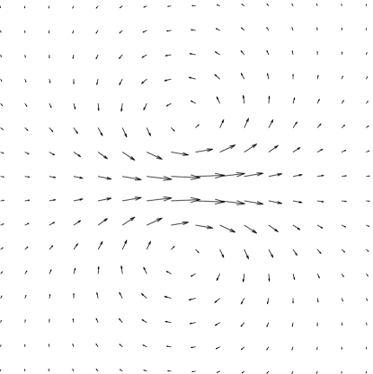
Figure 1. The dipole given by the kernel $K_{0,\eta}$ in dimension 2.

Finally we may also consider the limiting case $\varepsilon=0,\eta>0$. In this case $v=G_{\eta}^{(p)}\ast P_{\operatorname{div}=0}(m)$ so $v$ has divergence zero. There is no $L$ because $v$ determines $m$ only up to a gradient field. However EPDiff in Oseledets’s form form (5) makes perfect sense. Like Euler’s equation it gives geodesics on the group of volume preserving diffeomorphisms. As always, the energy is $E=\int v\cdot m$ and this is conserved on geodesics. Even though we have no $L$, we can rewrite the energy using $(I-\frac{\eta^{2}}{p}\triangle)^{p}v=P_{\operatorname{div}=0}(m)$, giving us:

$$E=\int v\cdot m=\int v\cdot P_{\operatorname{div}=0}(m)=\int v\cdot(I-\tfrac{\eta^{2}}{p}\triangle)^{p}v.$$

Alternatively, we may use the above energy to define a metric on the group of volume preserving diffeomorphisms which differ from the identity by a mapping in $H^{\infty}$ (or $\mathcal{S}$), and our equation is just the geodesic equation on $\operatorname{SDiff}_{H^{\infty}}(\mathbb{R}^{n})$ for this metric. Note that the Lie algebra of $\operatorname{SDiff}_{H^{\infty}}(\mathbb{R}^{n})$ is just the space of vector fields $v$ in $H^{\infty}$ with divergence zero and its dual is the space of 1-forms in $H^{\infty}$ modulo closed 1-forms, which is the same as the space of exact 2-forms in $H^{\infty}$. In the divergence free setting there is no need to consider 1-forms tensored with the standard density $dx$. On $\operatorname{SDiff}_{H^{\infty}}(\mathbb{R}^{n})$, the ‘momentum’ associated to a geodesic, defined as the dual of the tangent to the geodesic, is the classical vorticity of the flow and, in our formulation, we have simply ‘lifted’ this to the dual Lie algebra of $\operatorname{Diff}_{H^{\infty}}(\mathbb{R}^{n})$.

The case $p=1$ has been introduced and studied by Holm and collaborators (see [8], equation (8.29)) who use the letter $\alpha$ for our $\eta$ and call EPDiff the $\alpha$-Euler equation:

$$(1-\alpha^{2}\triangle)(\partial_{t}v) =-(v\cdot\nabla)(1-\alpha^{2}\triangle)v-(1-\alpha^{2}\triangle)v\cdot(Dv)^{t}+\nabla p,$$

$$\operatorname{div}(v) =0.$$

You can also drop incompressibility and when $n=1$ this becomes the Camassa-Holm equation [5].

The $K$ for the $\varepsilon=0,\eta>0$ metric is just the convolution $G^{(p)}_{\eta}\ast P_{\operatorname{div}=0}$. This $K$ can be explicitly calculated using the fact that the Green’s function $H$ is harmonic. We use:

Theorem 1.

Let $F(x)=f(|x|)$ be any integrable $C^{2}$ radial function on $\mathbb{R}^{n}$. Assume $n\geq 3$. Define:

$$H_{F}(x)=\int_{\mathbb{R}^{n}}\!\!\!\!\min\left(\tfrac{1}{|x|^{n-2}},\tfrac{1}{|y|^{n-2}}\right)F(y)dy=\frac{1}{|x|^{n-2}}\int_{|y|\leq|x|}\!\!\!\!F(y)dy+\int_{|y|\geq|x|}\!\!\frac{F(y)}{|y|^{n-2}}dy$$

Then $H_{F}$ is the convolution of $F$ with $\frac{1}{|x|^{n-2}}$, is in $C^{4}$ and:

$$\partial_{i}(H_{F})(x) =-(n-2)\frac{x_{i}}{|x|^{n}}\int_{|y|\leq|x|}\!\!\!\!F(y)dy$$

$$\partial_{i}\partial_{j}(H_{F})(x) =(n-2)\left(\frac{nx_{i}x_{j}-\delta_{ij}|x|^{2}}{|x|^{n+2}}\int_{|y|\leq|x|}\!\!\!\!F(y)dy-V_{n}\frac{x_{i}x_{j}}{|x|^{2}}F(x)\right)$$

If $n=2$, the same holds if you replace $1/|x|^{n-2}$ by $\log(1/|x|)$ and omit the factors $(n-2)$ in the derivatives.

Proof.

The idea is to first check that $H_{F}\in C^{2}$ with the above expressions for its first and second derivatives. This is straightforward when $x\neq 0$. Near $0$, let $F(x)=a+b|x|^{2}+o(|x|^{2})$. Then one checks that:

$$H_{F}(x)=\left(\int\frac{F(y)}{|y|^{n-2}}dy\right)-\frac{(n-2)aV_{n}}{2n}|x|^{2}-\frac{(n-2)bV_{n}}{4(n+2)}|x|^{4}+o(|x|^{4})$$

hence the expressions for the first and second derivatives extend across the origin. Taking the trace of the matrix of second derivatives, one finds that; $\triangle H_{F}=-(n-2)V_{n}F.$ Since the Green’s function of $-\triangle$ is $1/(n-2)V_{n}|x|^{n-2}$, this implies that $H_{F}$ is the convolution $F\ast(1/|x|^{n-2})$. ∎

This applies to $F=G^{(p)}_{\eta}$ for example, or to the limiting case where $F$ is a Gaussian, giving the following expression for the kernel $K_{0,\eta}$ for finite $p$ or the limiting Gaussian case:

(8) $$K_{0,\eta}(x)=\frac{\delta_{ij}|x|^{2}-x_{i}x_{j}}{|x|^{2}}G^{(p)}_{\eta}(x)+\frac{x_{i}x_{j}-\delta_{ij}|x|^{2}/n}{|x|^{2}}\text{Mean}_{B_{|x|}}\left(G^{(p)}_{\eta}\right)$$

where $B_{a}$ is the ball of radius $a$ centered at the origin.

We can summarize all possibilities in a handy table (we have changed notation slightly to use double subscripts $\varepsilon,\eta$ for all cases):

$$\boxed{\begin{array}[]{ll}\text{no }L&K_{0,0}=P_{\operatorname{div}=0}=\delta_{ij}\delta_{0}+(\partial_{i}\partial_{j}H)_{\text{distr}}\\ \text{no }L&K_{0,\eta}=G^{(p)}_{\eta}\ast P_{\operatorname{div}=0}\text{ -- see above}\\ L_{\varepsilon,0}=I-\tfrac{1}{\varepsilon^{2}}\nabla\circ\operatorname{div}&K_{\varepsilon,0}=\delta_{ij}\delta_{0}+\partial_{i}\partial_{j}H_{\varepsilon}\\ L_{\varepsilon,\eta}=\left(I-\tfrac{\eta^{2}}{p}\triangle\right)^{p}\circ\left(I-\tfrac{1}{\varepsilon^{2}}\nabla\circ\operatorname{div}\right)&K_{\varepsilon,\eta}=\delta_{ij}G^{(p)}_{\eta}+\partial_{i}\partial_{j}(G^{(p)}_{\eta}\ast H_{\varepsilon})\end{array}}$$

3. Existence theorems for the $L_{\varepsilon,\eta}$ metric

It is well known that local solutions of Euler’s equation itself, that is $L_{0,0}$, exist, e.g. see [11, 21]. Moreover global solutions of the EPDiff equations $L_{\varepsilon,\eta},\varepsilon,\eta>0,p\geq(n+3)/2$ have been shown to exist by Trouvé and Younes (unpublished but apparently implicit in the results of [22] for geodesics in what they call ‘metamorphosis’). Their result extends easily to the EPDiff equations $L_{0,\eta}$ because the kernel $K_{0,\eta}$ is still $C^{1}$, which holds so long as $p\geq(n+3)/2$. The method here is based on the Lagrangian form (3) of EPDiff. For completeness, we include the proof:

Theorem 2.

Let $\varepsilon\geq 0,\eta>0,p\geq(n+3)/2$ and $K=K_{\varepsilon,\eta}$ be the corresponding kernel. For any vector-valued distribution $m_{0}$ whose components are finite signed measures, consider the Lagrangian equation for a time varying $C^{1}$-diffeomorphism $\varphi(\cdot,t)$ with $\varphi(x,0)\equiv x$:

$$\partial_{t}\varphi(x,t)=\int K(\varphi(x,t)-\varphi(y,t))(D\varphi(y,t))^{-1,\top}m_{0}(y)dy.$$

Here $D\varphi$ is the spatial derivative of $\varphi$. This equation has a unique solution for all time $t$.

Proof.

The Eulerian velocity at $\varphi$ is:

$$V_{\varphi}(x)=\int K(x-\varphi(y))(D\varphi(y))^{-1,\top}m_{0}(y)dy$$

and $W_{\varphi}(x)=V_{\varphi}(\varphi(x))$ is the velocity in ‘material’ coordinates. Note that because of our assumption on $m_{0}$, if $\varphi$ is a $C^{1}$-diffeomorphism, then $V_{\varphi}$ and $W_{\varphi}$ are $C^{1}$ vector fields on $\mathbb{R}^{n}$; in fact, they are as differentiable as $K$ is, for suitably decaying $m$. The equation can be viewed as a the flow equation for the vector field $\varphi\mapsto W_{\varphi}$ on the union of the open sets

$$U_{c}=\big{\{}\varphi\in C^{1}(\mathbb{R}^{n})^{n}:\|\operatorname{Id}-\varphi\|_{C^{1}}<1/c,\;\det(D\varphi)>c\big{\}},$$

where $c>0$. The union of all $U_{c}$ is the group $\operatorname{Diff}_{C^{1}_{b}}(\mathbb{R}^{n})$ of all $C^{1}$-diffeomorphisms which, together with their inverses, differ from the identity by a function in $C^{1}(\mathbb{R}^{n})^{n}$ with bounded $C^{1}$-norm. We claim this vector field is locally Lipschitz on each $U_{c}$:

$$\|W_{\varphi_{1}}-W_{\varphi_{2}}\|_{C^{1}}\leq C.\|\varphi_{1}-\varphi_{2}\|_{C^{1}}$$

where $C$ depends only on $c$. This is easy to verify using the fact that $K$ is uniformly continuous and using $\|D\varphi^{-1}\|\leq\|D\varphi\|^{n-1}/|\det(D\varphi)|$. As a result we can integrate the vector field for short times in $\operatorname{Diff}_{C^{1}_{b}}(\mathbb{R}^{n})$. But since $(D\varphi(y,t))^{-1,\top}m_{0}(y)$ is then again a signed finite $\mathbb{R}^{n}$-valued measure,

$$\int V_{\varphi(\cdot,t)}(x)(D\varphi(y,t))^{-1,\top}m_{0}(y)dx=\|V_{\varphi(\cdot,t)}\|_{L_{\varepsilon,\eta}}$$

is actually finite for each $t$. Using the fact that in EPDiff the $L_{\varepsilon,\eta}$-energy $\|V_{\varphi(\cdot,t)}\|_{L_{\varepsilon,\eta}}$ of the $L_{\varepsilon,\eta}$-geodesic is constant in $t$, we get a bound on the norm $\|V_{\varphi(\cdot,t)}\|_{H^{p}}$, depending of course on $\eta$ but independent of $t$, hence a bound on $\|V_{\varphi(\cdot,t)}\|_{C^{1}}$. Thus $\|\varphi(\cdot,t)\|_{C^{0}}$ grows at most linearly in $t$. But $\partial_{t}D\varphi=DW_{\varphi}=DV_{\varphi}\cdot D\varphi$ which shows us that $D\varphi$ grows at most exponentially in $t$. Hence $\det D\varphi$ can shrink at worst exponentially towards zero, because $\partial_{t}\det(D\varphi)=\operatorname{Tr}(\operatorname{Adj}(D\varphi).\partial_{t}D\varphi)$. Thus for all finite $t$, the solution $\varphi(\cdot,t)$ stays in a bounded subset of our Banach space and the ODE can continue to be solved. ∎

For $L_{\varepsilon,0}$ with $\varepsilon>0$ we proved in a previous paper [14] that the $L_{\varepsilon,0}$-metric defined a well behaved Riemannian metric on the group of diffeomorphisms of $\mathbb{R}^{n}$ in that the infimum of path lengths joining two distinct diffeomorphisms was positive. Here we prove that for all $\varepsilon$ and $\eta$, including $\varepsilon=0$ and/or $\eta=0$, geodesics exist locally – though as in the Euler case, as far as we know, they might become singular in finite time hence not be indefinitely prolongable – and that these local solutions behave continuously in the parameters $\varepsilon,\eta$. In particular, as $\varepsilon,\eta\rightarrow 0$ they approach solutions of Euler’s equation.

Everything depends on proving a Sobolev estimate for the time derivative of certain energies. We need the following straightforward lemma:

Lemma.

If $\eta\geq 0$ and $\varepsilon>0$ are bounded above, then the norm

$$\|v\|_{k,\varepsilon,\eta}^{2}=\sum_{|\alpha|\leq k}\int\langle D^{\alpha}L_{\varepsilon,\eta}v,D^{\alpha}v\rangle dx$$

is bounded above and below by the metric, with constants independent of $\varepsilon$ and $\eta$:

$$\|v\|_{H^{k}}^{2}+\tfrac{1}{\varepsilon^{2}}\|\mathrm{div}(v)\|_{H^{k}}^{2}+\sum_{k+1\leq|\alpha|\leq k+p}\eta^{2(|\alpha|-k)}\int|D^{\alpha}v|^{2}+\tfrac{1}{\varepsilon^{2}}|D^{\alpha}\mathrm{div}(v)|^{2}$$

Here $H^{k}$ is the $k^{th}$ order Sobolev norm for the standard metric, and $D^{\alpha}$ is the partial derivative for the multiindex $\alpha$. We also often omit $dx$ at the end of integrals, and corresponding brackets. The proof of the lemma is obvious by expanding $L_{\varepsilon,\eta}$.

Assuming $k$ is sufficiently large, for instance $k\geq(n+2p+4)$ works, we now prove the main estimate:

$$\boxed{|\partial_{t}\left(\|v\|^{2}_{k,\varepsilon,\eta}\right)|\leq C.\|v\|_{k,\varepsilon,\eta}^{3}}$$

where, so long $\varepsilon$ and $\eta$ are bounded above, the constant $C$ is independent of $\varepsilon$ and $\eta$.

Write $M_{\eta}=(I-\tfrac{\eta^{2}}{p}\triangle)^{p}$, so that $m_{i}=M_{\eta}v_{i}-\tfrac{1}{\varepsilon^{2}}M_{\eta}\operatorname{div}(v)_{,i}$. Using EPDiff and integration by parts, the time derivative is given by:

$$\tfrac{1}{2}\partial_{t}\left(\|v\|^{2}_{k,\varepsilon,\eta}\right) =\sum_{|\alpha|\leq k}\int_{\mathbb{R}^{n}}(\partial_{t}D^{\alpha}m,D^{\alpha}v)$$

$$=\sum_{i,j,|\alpha|\leq k}\int_{\mathbb{R}^{n}}(-1)^{|\alpha|+1}D^{2\alpha}v_{i}.\left(v_{j}.m_{i,j}+m_{i}.v_{j,j}+m_{j}.v_{j,i}\right)$$

Next replace the $m_{i}$ by $M_{\eta}v_{i}-\tfrac{1}{\varepsilon^{2}}M_{\eta}\operatorname{div}(v)_{,i}$. Integrating the third term by parts to move the $i^{th}$ derivative of $v_{j}$ to the other factors and noting that the two terms involving the second derivative of $\operatorname{div}\,v$ cancel, one checks that the estimate can be reduced to 6 terms all of the form $\int D^{2\alpha}f\cdot g\cdot M_{\eta}h$ with one of the triples:

$$(f,g,h)= (v_{i},v_{j},v_{i,j}), (v_{i},v_{j},v_{j,i}), (v_{i},\operatorname{div}\,v,v_{i}),$$

$$(\tfrac{\operatorname{div}\,v}{\varepsilon},v_{j},\tfrac{\operatorname{div}\,v_{,j}}{\varepsilon}), (v_{i},\tfrac{\operatorname{div}\,v}{\varepsilon},\tfrac{\operatorname{div}\,v_{,i}}{\varepsilon}), (\operatorname{div}\,v,v_{j},v_{j}).$$

Next we expand $M_{\eta}$ to $\sum_{|\beta|\leq p}(-1)^{|\beta|}\frac{\eta^{2|\beta|}}{p^{|\beta|}}D^{2\beta}$ (omitting binomial constants) and integrate by parts some more, moving a $D^{\alpha}$ from the first to second or third terms and a $D^{\beta}$ from the third to first or second terms, getting terms

$$\frac{\eta^{2|\beta|}}{p^{|\beta|}}\int D^{\alpha+\beta_{1}}f\cdot D^{\alpha_{2}+\beta_{2}}g\cdot D^{\beta+\alpha_{1}}h$$

where $\alpha=\alpha_{1}+\alpha_{2},\beta=\beta_{1}+\beta_{2}$. Now either $\alpha_{1}$ or $\alpha_{2}$ is less than or equal to $k/2$ so that the corresponding (second or third) term in the integrand has order at most $k/2+p+1$, hence $\leq k-n/2-1$. Thus by the Sobolev inequalities, its sup norm is bounded by its $k^{th}$ Sobolev norm and we have:

$$\frac{\eta^{2|\beta|}}{p^{|\beta|}}\Big{|}\int D^{\alpha+\beta_{1}}f\cdot D^{\alpha_{2}+\beta_{2}}g\cdot D^{\beta+\alpha_{1}}h\Big{|}\leq\\ \leq\frac{1}{p^{|\beta|}}\left\{\begin{array}[]{ll}\|\eta^{|\beta|}D^{\alpha+\beta_{1}}f\|_{L^{2}}\cdot\|g\|_{H^{k}}\cdot\|\eta^{|\beta|}D^{\beta+\alpha_{1}}h\|_{L^{2}},&\text{if }|\alpha_{2}|\leq k/2,\\ \|\eta^{|\beta|}D^{\alpha+\beta_{1}}f\|_{L^{2}}\cdot\|\eta^{|\beta|}D^{\alpha_{2}+\beta_{2}}g\|_{L^{2}}\cdot\|h\|_{H^{k}},&\text{if }|\alpha_{1}|\leq k/2.\end{array}\right.$$

The first term is always bounded by $\|f\|_{k,\varepsilon,\eta}$ and so is the other $D$-term except in the first case with $\alpha_{2}=0,|\alpha|=k,|\beta|=p$ and $h$ is a first derivative $\tilde{h}_{,\ell}$ with $\tilde{h}$ either a component of $v$ or $\operatorname{div}\,v/\varepsilon$. In this last case, the third term has $k+p+1$ derivatives, so the lemma does not apply. But we can still integrate by parts, putting the $\ell^{\text{th}}$ derivative on the other terms. If $|\beta_{2}|>0$ or if $f=v_{\ell}$, this reduces again to terms bounded by the $(k,\varepsilon,\eta)$ norm. The only remaining case is when $f=\tilde{h}$, and then we have:

$$\int D^{\alpha+\beta}f\cdot g\cdot D^{\alpha+\beta}f_{,\ell}=\tfrac{1}{2}\int(D^{\alpha+\beta}f)^{2}_{,\ell}\cdot g=-\tfrac{1}{2}\int(D^{\alpha+\beta}f)^{2}\cdot g_{,\ell}$$

and this finishes the proof of the estimate.

Using this estimate, we can prove:

Theorem 3.

Fix $k,p,n$ with $p>n/2+1,k\geq n+2p+4$ and assume $(\varepsilon,\eta)\in[0,M]^{2}$ for some $M>0$. Then there are constants $t_{0},C$ such that for all initial conditions $v_{0}\in H^{k+p+1}$, there is a unique solution $v_{\varepsilon,\eta}(x,t)$ of the above case of EPDiff (including the limiting case of Euler’s equation) for $t\in[0,t_{0}]$. The solution $v_{\varepsilon,\eta}(\cdot,t)\in H^{k+p+1}$ depends continuously on $\varepsilon,\eta\in[0,M]^{2}$ and satisfies $\|v_{\varepsilon,\eta}(\cdot,t)\|_{k,\varepsilon,\eta}<C$ for all $t\in[0,t_{0}]$.

For $\varepsilon,\eta>0$, existence and uniqueness for all time has been proven in [22]. Their proof has been extended to the case $\varepsilon=0,\eta>0$ in Theorem 2. For $\varepsilon=\eta=0$, this is the well known result for Euler’s equation. What remains is the new case $\varepsilon>0,\eta=0$. We follow a standard approach, used, for example, in [21], Ch. 16 and 17. First consider existence. But by our estimate and Gronwall’s lemma, we have a local upper bound uniformly in $\varepsilon,\eta$ for these solutions:

$$\|v_{\varepsilon,\eta}\|_{k,\varepsilon,\eta}\leq C(t),t\in[0,t_{0}].$$

But, for $k,p$ as above, by the lemma we have $\|v\|_{H^{k}}\leq C_{1}\|v\|_{k,\varepsilon,\eta}$ with $C_{1}$ independent of $\varepsilon,\eta$. Thus the Hilbert space with the norm $\|\cdot\|_{k,\varepsilon,\eta}$ is compactly embedded in $C^{1}(\mathbb{R}^{n})$ in the local sense that any bounded sequence for the former has a subsequence which, for every compact subset $K\subset\mathbb{R}^{n}$, converges in $C^{1}(K)$. Therefore $v_{\varepsilon,\eta}(t)$ lie in a ‘locally’ compact part of the Banach space of $C^{1}$ functions of $(x,t)$. Therefore, as $\varepsilon$ or $\eta$ tend to zero, they have a convergent subsequence whose limit $v$ must be a solution of the corresponding EPDiff, because each equation can be written in terms of the corresponding kernel, and the kernels depend nicely on $\varepsilon$ and $\eta$. So by Gronwall’s lemma again the original estimates gives $H^{k}$ bounds on this solution.

Next we prove that the cluster point for $\varepsilon\to 0$ or $\eta\to 0$ of the solutions $v_{\varepsilon,\eta}$ is unique. Let us temporarily abbreviate $L_{\varepsilon,0}$ by $L$ and let $v$ and $\widetilde{v}$ be two solutions of EPDiff for this $L$. We write $u=v-\widetilde{v}$ for their difference and follow the ideas of the preceding estimate to estimate $\tfrac{d}{dt}\|u\|^{2}_{L}$.

$$\tfrac{d}{dt}\|u\|^{2}_{L} =2\int\langle\tfrac{d}{dt}Lu,u\rangle dx\qquad\text{so using summation of indices:}$$

$$=-2\int u_{i}\cdot\left(v_{j}Lv_{i,j}+Lv_{i}\,\operatorname{div}v+Lv_{j}v_{j,i}-\widetilde{v}_{j}L\widetilde{v}_{i,j}-L\widetilde{v}_{i}\,\operatorname{div}\widetilde{v}-L\widetilde{v}_{j}\widetilde{v}_{j,i}\right)$$

$$=-2\int u_{i}\left(u_{j}Lv_{i,j}+\widetilde{v}_{j}Lu_{i,j}+Lu_{i}\,\operatorname{div}v+L\widetilde{v}_{i}\,\operatorname{div}u+Lv_{j}u_{j,i}+Lu_{j}\widetilde{v}_{j,i}\right)$$

Next replace all expressions of the form $Lu_{k}$ by $u_{k}-\tfrac{1}{\varepsilon^{2}}\partial_{k}\operatorname{div}u$. Then integrate by parts by the “div” part of the last term, that is replace $-u_{i}\cdot\tfrac{1}{\varepsilon^{2}}(\operatorname{div}u)_{,j}\widetilde{v}_{j,i}$ by

$$u_{i}\cdot\tfrac{1}{\varepsilon^{2}}(\operatorname{div}u)_{,ij}\widetilde{v}_{j}+\operatorname{div}u\cdot\tfrac{1}{\varepsilon^{2}}(\operatorname{div}u)_{,j}\widetilde{v}_{j}$$

The term with the second derivative of $\operatorname{div}v$ cancels the term with the second derivative of $\operatorname{div}v$ arising from the second term $\widetilde{v}_{j}Lu_{i,j}$ in the above expression. With this and further integration by parts, we get:

$$\tfrac{d}{dt}\|u\|^{2}_{L} =-2\int u_{i}u_{j}(Lv_{i,j}+\widetilde{v}_{j,i})+u_{i}^{2}\operatorname{div}v+u_{i}u_{i,j}\widetilde{v}_{j}+u_{i}u_{j,i}Lv_{j}+$$

$$\qquad\qquad+u_{i}\,\operatorname{div}u\,L\widetilde{v}_{i}+\tfrac{1}{\varepsilon^{2}}(\operatorname{div}u)_{,i}(\operatorname{div}u\,\widetilde{v}_{i}-u_{i}\operatorname{div}v)$$

$$=-2\int u_{i}u_{j}(Lv_{i,j}-Lv_{j,i}+\widetilde{v}_{j,i})+u_{i}^{2}(\operatorname{div}v-\tfrac{1}{2}\operatorname{div}\widetilde{v})+$$

$$\qquad\qquad+u_{i}\,\operatorname{div}u\,(L\widetilde{v}_{i}-Lv_{i}+\tfrac{1}{\varepsilon^{2}}\operatorname{div}(v)_{,i})+\tfrac{1}{\varepsilon^{2}}(\operatorname{div}u)^{2}(\operatorname{div}v-\tfrac{1}{2}\operatorname{div}\widetilde{v})$$

$$\leq C.\|u\|^{2}_{L}$$

where the constant depends on the strong sup bounds we have for $v$ and $\widetilde{v}$. By Gronwall again, this means that we have a growth estimate on $\|u\|^{2}_{L}$ as a function of $t$. In particular, if $u$ is zero at time 0, it is always zero and this proves uniqueness.

Finally, as $\varepsilon$ goes to zero, we again have the solutions lying in a ‘locally’ compact part of $C^{1}$ (as above) so if there is only possible limit, they must converge to this limit and are continuous in $\eta$. Likewise, as $\varepsilon$ converges to zero, this solution must converge to that of Euler’s equation.

4. Conserved quantities: linear and angular momentum

We would like to derive the conservation laws from Noether’s theorem using the fact that our geodesic equation is invariant with respect to the Euclidean group $SO(n)\ltimes\mathbb{R}^{n}$, as we did in our earlier paper [15]. However, if we take $(X,w)\in\mathfrak{s}\mathfrak{o}(n)\ltimes\mathbb{R}^{n}$ to be the infinitesimal generator for the 1-parameter group $(\exp(tX),tw)$, composition maps a diffeomorphism $\varphi\in\operatorname{Diff}_{\mathcal{S}}(\mathbb{R}^{n})$ to the diffeomorphsm $\exp(tX)\circ\,\varphi+tw$. Unfortunately, the latter diffeomorphism no longer rapidly falls towards $\operatorname{Id}_{\mathbb{R}^{n}}$ so it is not in $\operatorname{Diff}_{\mathcal{S}}(\mathbb{R}^{n})$. The infinitesimal generator for this action is

$$\zeta_{(X,w)}(\varphi)=\partial_{t}|_{0}(\exp(tX)\circ\,\varphi+tw)=X\circ\,\varphi+w.$$

Consider a right invariant Riemannian metric $G$ on $\operatorname{Diff}_{\mathcal{S}}(\mathbb{R}^{n})$ as described for example in [13], so that $G_{\varphi}$ is an inner product on the tangent space at $\varphi$, which is invariant under the motion group. Then for any geodesic $t\mapsto\varphi(\cdot,t)$ the right invariant inner product $G_{\varphi}(\zeta_{(X,w)}(\varphi),\varphi_{t})$ should constant in $t$, according to Noether’s theorem in the form of [3, section 2.6], if the action above was a left action of the motion group on $\operatorname{Diff}_{\mathcal{S}}(\mathbb{R}^{n})$. We could dedure this directly by taking $\operatorname{Diff}_{\mathcal{S}}(\mathbb{R}^{n})$ as the normal subgroup of an extension of the motion group which can be described as a group of diffeomorphisms which fall rapidly to “Euclidean motions near infinity” and extend the metric to a right invariant one. Instead of doing this in detail we directly check that the the above well defined expression is indeed constant in $t$ along each geodesic. Note first that

$$G_{\varphi}(\zeta_{(X,w)}(\varphi),\varphi_{t}) =G_{\varphi}(X\circ\,\varphi,\varphi_{t})+G_{\varphi}(w,\varphi_{t})$$

$$=G_{\operatorname{Id}}(X,\varphi_{t}\circ\,\varphi^{-1})+G_{\operatorname{Id}}(w,\varphi_{t}\circ\,\varphi^{-1})$$

$$=G_{\operatorname{Id}}(X,v)+G_{\operatorname{Id}}(w,v)\quad\text{ where }\varphi_{t}(\cdot,t)=v(\varphi(\cdot,t),t)$$

$$=\int\langle X.x,L(v)(x)\rangle\,dx+\int\langle w,L(v)(x)\rangle\,dx$$

$$=\int(X.x,\widetilde{m}(x))+\int(w,\widetilde{m}(x));$$

the first expression viewed as a linear functional in $X\in\mathfrak{s}\mathfrak{o}(n)$ is the $\mathfrak{s}\mathfrak{o}(n)^{*}$-valued angular momentum mapping. If we identify $\mathfrak{s}\mathfrak{o}(n)^{*}$ with $\mathfrak{s}\mathfrak{o}(n)$ via the Killing form we can write the angular momentum succinctly as $\int x\wedge\widetilde{m}(x)$. Similarly the second expression leads to the linear momentum given by $\int\widetilde{m}(x)$.

Let us finally prove that these momenta are conserved by the geodesic flow. We shall use the geodesic equation in the form $\partial_{t}\widetilde{m}=-\mathcal{L}_{v}\widetilde{m}$. Then we have

$$\partial_{t}\int(X.x,\widetilde{m}(x)) =\int(X.x,\partial_{t}\widetilde{m}(x))=-\int(X,\mathcal{L}_{v}\widetilde{m})$$

$$=\int(\mathcal{L}_{v}X,\widetilde{m})=\int([v,X],\widetilde{m})=\int(-\mathcal{L}_{X}v,\widetilde{m})$$

$$=-\int\langle\mathcal{L}_{X}v,Lv\rangle dx\qquad\text{ now use }\mathcal{L}_{X}(L)=0\text{ and }\mathcal{L}_{X}(dx)=0,$$

$$=-\int\tfrac{1}{2}\mathcal{L}_{X}(\langle v,Lv\rangle dx)=0.$$

For the linear momentum the proof is similar.

5. Explicit bounds on the approximation I

Assume you start with the same initial condition $v(x,0)$ and integrate with both Euler’s equation and EPDiff with $L_{\varepsilon,\eta}$. Exactly how close are they? If you look at the kernels $K_{\varepsilon,\eta}$, you see that the effect of $\varepsilon>0$ is to shrink the tails of $K$ from polynomial to exponential and, correspondingly, to eliminate the pole of its Fourier transform at zero. On the other hand, the effect of $\eta>0$ is to smooth the singularity of $K$ at zero or to suppress the high frequencies in its Fourier transform. These being opposite operations, we need to estimate their effects separately. In this section, we consider the case $\eta=0$ and compare Euler’s equation with that given by $L_{\varepsilon,0}$. Let $v_{0}(x,t)$ be the solution of Euler’s equation and let $v_{\varepsilon}(x,t)$ be the solution of EPDiff with $L_{\varepsilon,0}$ (below abbreviated to $L_{\varepsilon}$). Our goal is to prove the theorem:

Theorem 4.

Take any $k$ and $M$ and any smooth initial velocity $v(\cdot,0)$. Then there are constants $t_{0},C$ such that Euler’s equation and $(\varepsilon,0)$-EPDiff have solutions $v_{0}$ and $v_{\varepsilon}$ respectively for $t\in[0,t_{0}]$ and all $\varepsilon<M$ and these satisfy:

$$\|v_{0}(\cdot,t)-v_{\varepsilon}(\cdot,t)\|_{H^{k}}\leq C\varepsilon.$$

Note that by Theorem 3 we have essentially any bound we need on both $v_{0}$ and $v_{\varepsilon}$. The $t_{0}$ is needed only to guarantee the bounds on the solutions derived in Theorem 3 hold for a big enough $k$ to give us the needed bounds. As above the proof is based on an estimate of the form:

(9) $$\partial_{t}\left(\|v_{0}-v_{\varepsilon}\|^{2}_{H^{k}}\right)\leq C_{1}\|v_{0}-v_{\varepsilon}\|^{2}_{H^{k}}+\varepsilon C_{2}\|v_{0}-v_{\varepsilon}\|_{H^{k}}$$

where $C_{1}$ and $C_{2}$ depend on the initial condition $v(\cdot,0)$ and $k$ but not on $\varepsilon$ at all times $t$ for which Theorem 3 holds for needed norm bounds on $v_{0}$ and $v_{\varepsilon}$.

Let $u=v_{0}-v_{\varepsilon}$ and calculate as follows, using the geodesic equation (7) for $L_{\varepsilon}$:

$$\tfrac{1}{2}\partial_{t} (\|u\|_{H^{k}}^{2})=\sum_{|\alpha|\leq k}\int D^{\alpha}u\cdot(D^{\alpha}(\partial_{t}v_{0}-\partial_{t}v_{\varepsilon}))$$

$$=\sum_{|\alpha|\leq k}\int D^{\alpha}u\cdot D^{\alpha}\Big{\{}-K_{0}\ast(v_{0}\cdot\nabla)v_{0}$$

$$\quad+K_{\varepsilon}\ast(v_{\varepsilon}\cdot\nabla)v_{\varepsilon}+v_{\varepsilon}\cdot\operatorname{div}(v_{\varepsilon})+\tfrac{\varepsilon^{2}}{2}(\nabla H_{\varepsilon})\ast|v_{\varepsilon}(x)|^{2}+\tfrac{1}{2}(\nabla H_{\varepsilon})\ast(\operatorname{div}v_{\varepsilon})^{2}\Big{\}}$$

$$\leq\sum_{|\alpha|\leq k}\|D^{\alpha}u\|_{L^{2}}\cdot\Big{\{}\|D^{\alpha}(K_{\varepsilon}-K_{0})\ast(v_{\varepsilon}\cdot\nabla)v_{\varepsilon}\|_{L^{2}}+\|D^{\alpha}(v_{\varepsilon}\cdot\operatorname{div}(v_{\varepsilon}))\|_{L^{2}}$$

$$\quad+\|D^{\alpha}(\tfrac{\varepsilon^{2}}{2}(\nabla H_{\varepsilon})\ast|v_{\varepsilon}|^{2})\|_{L^{2}}+\|D^{\alpha}(\tfrac{1}{2}(\nabla H_{\varepsilon})\ast(\operatorname{div}v_{\varepsilon})^{2})\|_{L^{2}}$$

$$\quad+\|K_{0}\ast D^{\alpha}((u\cdot\nabla)v_{\varepsilon})\|_{L^{2}}\Big{\}}-\sum_{|\alpha|\leq k}\int D^{\alpha}u\cdot K_{0}\ast D^{\alpha}((v_{0}\cdot\nabla)u)$$

$$\leq\|u\|_{H^{k}}\cdot\Big{\{}\|(K_{0}-K_{\varepsilon})\ast(v_{\varepsilon}\cdot\nabla)v_{\varepsilon}\|_{H^{k}}+\|v_{\varepsilon}\cdot\operatorname{div}(v_{\varepsilon})\|_{H^{k}}$$

$$\quad+\|\tfrac{\varepsilon^{2}}{2}\nabla H_{\varepsilon}\ast|v_{\varepsilon}|^{2}\|_{H^{k}}+\|\tfrac{1}{2}\nabla H_{\varepsilon}\ast(\operatorname{div}v_{\varepsilon})^{2}\|_{H^{k}}$$

(10) $$\quad+\|((v_{0}-v_{\varepsilon})\cdot\nabla)v_{\varepsilon}\|_{H^{k}}\Big{\}}-\sum_{|\alpha|\leq k}\int D^{\alpha}(v_{0}-K_{0}\ast v_{\varepsilon})\ast D^{\alpha}((v_{0}\cdot\nabla)u)$$

Here, in the last line, we used the fact that $K_{0}$, being an orthogonal projection, has norm 1 and is self-adjoint. Likewise $K_{\varepsilon}$, after Fourier transform, at frequency $\xi$, is multiplication by a diagonal matrix with eigenvalues 1 and $\varepsilon^{2}/(\varepsilon^{2}+|\xi|^{2})$; hence is also a bounded self-adjoint operator with norm 1.

For the first term, if we abbreviate $v_{\varepsilon}$ to $v$, first write:

$$\left((K_{0}-K_{\varepsilon})\ast(v\cdot\nabla)v\right) =F-(K_{0}-K_{\varepsilon})\ast v\cdot\operatorname{div}(v)$$

$$\text{where }F_{i} =\sum_{j,k}(K_{0}-K_{\varepsilon})_{ij}\ast(v_{j}v_{k})_{,k}=\sum_{j,k}\partial_{k}(K_{0}-K_{\varepsilon})_{ij}\ast v_{j}v_{k}$$

The Fourier transform of the derivative of the difference of the $K$’s is:

$$\left(\partial_{k}(K_{0}-K_{\varepsilon})_{ij}\right)\!\!\widehat{\vphantom{\big{)}}\hskip 10.84006pt}=\sqrt{-1}\xi_{i}\xi_{j}\xi_{k}\frac{\varepsilon^{2}}{|\xi|^{2}(\varepsilon^{2}+|\xi|^{2})}$$

Thus

$$\|F\|^{2}_{H^{k}} =\int(1+|\xi|^{2})^{k}\sum_{i}\left|\sum_{j,k}\tfrac{\varepsilon^{2}\xi_{i}\xi_{j}\xi_{k}}{|\xi|^{2}(\varepsilon^{2}+|\xi|^{2}}\widehat{v_{k}v_{j}}\right|^{2}$$

$$\leq\int(1+|\xi|^{2})^{k}\tfrac{\varepsilon^{4}}{|\xi|^{2}(\varepsilon^{2}+|\xi|^{2})^{2}}\sum_{j,k}(\xi_{j}\xi_{k})^{2}\cdot\sum_{j,k}|\widehat{v_{j}v_{k}}|^{2}|$$

$$\leq\int(1+|\xi|^{2})^{k}\tfrac{\varepsilon^{2}}{4}\sum_{j,k}|\widehat{v_{j}v_{k}}|^{2}=\tfrac{\varepsilon^{2}}{4}\sum_{j,k}\|v_{j}v_{k}\|^{2}_{H^{k}}$$

Repeating this for $v.\operatorname{div}(v)$ also, we find:

$$\|(K_{0}-K_{\varepsilon})\ast(v\cdot\nabla)v)\|_{H^{k}}\leq\tfrac{\varepsilon}{2}\sum_{j,k}\|v_{j}v_{k}\|_{H^{k}}+\|v\cdot\operatorname{div}(v)\|_{H^{k}})<C\varepsilon\|v\|_{k+m,\varepsilon,0}^{2}$$

for some universal constant $C$ coming from the product rule for Sobolev spaces and $m=\lceil n/4\rceil$. Along the way we also derived a similar bound for the second term in the expression (10).

To treat the third and fourth terms we need the bound on the norm of convolution with $\nabla H_{\varepsilon}$:

$$|\varepsilon\cdot\widehat{(H_{\varepsilon})_{,i}}|=\tfrac{\varepsilon|\xi_{i}|}{\varepsilon^{2}+|\xi|^{2}}\leq\tfrac{|\xi_{i}|}{2|\xi|},$$

hence $\|\varepsilon\nabla H_{\varepsilon}\ast f\|_{H^{k}}\leq\tfrac{1}{2}\|f\|_{H^{k}}$ for any function $f$ and in particular:

$$\|(\tfrac{\varepsilon^{2}}{2}\nabla H_{\varepsilon})\ast|v_{\varepsilon}(x)|^{2}\|_{H^{k}} \leq\tfrac{\varepsilon}{2}\||v_{\varepsilon}|^{2}\|_{H^{k}}\leq C\varepsilon\|v_{\varepsilon}\|_{k+m,\varepsilon,0}^{2}$$

$$\|(\tfrac{1}{2}\nabla H_{\varepsilon})\ast(\operatorname{div}v_{\varepsilon})^{2}\|_{H^{k}} \leq\tfrac{\varepsilon}{2}\|\left(\tfrac{\operatorname{div}v_{\varepsilon}}{\varepsilon}\right)^{2}\|_{H^{k}}\leq C\varepsilon\|v_{\varepsilon}\|_{k+m,\varepsilon,0}^{2}$$

For the fifth term in expression (10) we use sup bounds on $k+1$ derivatives of $v_{\varepsilon}$ and the Sobolev inequality to obtain:

$$\|(u\cdot\nabla)v_{\varepsilon}\|_{H^{k}}\leq C\|u\|_{H^{k}}\cdot\|v_{\varepsilon}\|_{H^{\ell}},\quad\text{with }\ell=k+1+\lceil\tfrac{n+1}{2}\rceil$$

We come to the last term in (10). Up to constants, we write it as:

(11) $$\sum_{0\leq\beta\leq\alpha,|\alpha|\leq k}\int D^{\alpha}u\cdot(D^{\beta}v_{0}\cdot\nabla)D^{\alpha-\beta}u+\int D^{\alpha}(v_{\varepsilon}-K_{0}\ast v_{\varepsilon})\cdot D^{\alpha}(v_{0}\cdot\nabla)u$$

In the first term of (11), the summand with $\beta=0$ vanishes because it equals $\int v_{0}\cdot\nabla(\tfrac{|D^{\alpha}u|^{2}}{2})$ and $v_{0}$ has zero divergence. Using a sup norm on $D^{\beta}v_{0}$, the remaining summands are bounded by $\|v_{0}-v_{\varepsilon}\|_{H^{k}}^{2}$ times this sup norm. This sup norm is bounded by a universal constant times $\|v_{0}\|_{H^{\ell}}$ with $\ell=k+\lceil\tfrac{n+1}{2}\rceil$. To bound the second term in (11), using the expression for $K_{0}$ we find $v_{\varepsilon}-K_{0}\ast v_{\varepsilon}=\nabla H_{0}\ast\operatorname{div}(v_{\varepsilon})$. Now calculate:

$$\int D^{\alpha}(v_{\varepsilon}-K_{0}\ast v_{\varepsilon})\cdot D^{\alpha}((v_{0}\cdot\nabla)u)=-\sum_{i,j}\int D^{\alpha}(\partial_{i}\partial_{j}H_{0}\ast\operatorname{div}(v_{\varepsilon}))\cdot D^{\alpha}((v_{0})_{i}u_{j})$$

But $\partial_{i}\partial_{j}H_{0}$ has Fourier transform $(\xi_{i}\xi_{j})/|\xi|^{2}$, a matrix with eigenvalues 0 and 1, so the $L^{2}$ norm of the first factor is bounded by $\varepsilon\|v_{\varepsilon}\|_{k,\varepsilon,0}$. Then, as above, we get a bound of the form:

$$C\varepsilon\|v_{\varepsilon}\|_{k,\varepsilon,0}\cdot\|v_{0}\|_{H^{\ell}}\cdot\|u\|_{H^{k}}$$

with $\ell=k+\lceil\tfrac{n+1}{2}\rceil$. Now using Theorem 3, we see that we can bound all needed norms of $v_{0}$ and $v_{\varepsilon}$ on this time interval by norms of the initial condition $v(\cdot,0)$. Putting everything together, we get the asserted bound (9).

To complete the proof of the Theorem, rewrite (9) in the form

$$\partial_{t}\|u\|_{H^{k}} \leq\frac{C_{2}}{2}\varepsilon+\frac{C_{1}}{2}\|u\|_{H^{k}}\quad\text{ or}$$

$$\|u(t)\|_{H^{k}} \leq\frac{C_{2}}{2}\varepsilon t+\int_{0}^{t}\frac{C_{1}}{2}\|u(s)\|_{H^{k}}ds$$

and apply Gronwall’s lemma to obtain $\|v_{0}(t)-v_{\varepsilon}(t)\|_{H^{k}}=\|u(t)\|_{H^{k}}\leq\varepsilon^{2}C_{3}e^{C_{1}t/2}=O(\varepsilon)$ as required.

In comparing Euler’s equation with EPDiff for $(\varepsilon,0)$, a key point is that $K_{0}=P_{\operatorname{div}=0}$ and $K_{\varepsilon}=K_{\varepsilon,0}$ have identical singularities at the origin, but their difference is much better behaved. In fact convolution with $K_{0}-K_{\varepsilon}$ equals

$$\nabla\circ(\text{convolution with }J_{\varepsilon})\circ\operatorname{div}$$

where $J_{\varepsilon}$ has Fourier transform $1/|\xi|^{2}(\varepsilon^{2}+|\xi|^{2})$. Near the origin, this looks like $e^{-|x|}$ in $\mathbb{R}^{3}$, has a log pole in $\mathbb{R}^{4}$ and is like $1/|x|^{n-4}$ in higher spaces. Considering Euler’s equation and EPDiff for $(\varepsilon,0)$ in Lagrangian form (3), they differ only by changing the convolution on the right hand side by this term. This makes it seems reasonable to conjecture that if solutions of $(\varepsilon,0)$-EPDiff do not blow up, i.e. exist for all time, then neither do the solutions to Euler’s equation. Or conversely, if Euler’s solutions do blow up, so do solutions of this EPDiff.

6. Explicit bounds on the approximation II

Now we want to compare solutions of EPDiff for $\varepsilon>0,\eta=0$ with solutions for $\varepsilon>0,\eta>0$. The difference here is a convolution with the Gaussian $G_{\eta}$, so solutions with $\eta>0$ are essentially just smoothed or low-pass version of those with $\eta=0$. We will prove:

Theorem 5.

Let $\varepsilon>0$. Take any $k$ and $M$ and any smooth initial velocity $v(\cdot,0)$. Then there are constants $t_{0},C$ such that $(\varepsilon,0)$-EPDiff and $(\varepsilon,\eta)$-EPDiff have solutions $v_{0}$ and $v_{\eta}$ respectively for $t\in[0,t_{0}]$ and all $\varepsilon,\eta<M$ and these satisfy:

$$\|v_{0}(\cdot,t)-v_{\eta}(\cdot,t)\|_{H^{k}}\leq C\eta^{2}.$$

A basic tool is the simple estimate:

(12) $$\|f-G_{\eta}^{(p)}\ast f\|_{L^{2}}\leq\eta^{2}\|\triangle f\|_{L^{2}}$$

To prove this, just take Fourier transforms and use the elementary inequality:

$$\left(1-(1+\tfrac{\eta^{2}}{p}|\xi|^{2})^{-p}\right)\leq\eta^{2}|\xi|^{2}.$$

Working as in the setup of Theorem 4, let $m_{0}$ and $m_{\eta}$ be the momenta corresponding to $v_{0}$ and $v_{\eta}$. Write $u=v_{0}-v_{\eta}$ and calculate the time derivative of:

$$\|u\|^{2}_{k,\varepsilon,0}=\sum_{|\alpha|\leq k}\int\langle D^{\alpha}u,D^{\alpha}L_{\varepsilon}u\rangle=\|u\|^{2}_{H^{k}}+\|\tfrac{\operatorname{div}(u)}{\varepsilon}\|^{2}_{H^{k}}.$$

We get a lot of terms:

$$\tfrac{1}{2}\partial_{t}\|u\|^{2}_{k,\varepsilon,0} =\sum_{|\alpha|\leq k}\int D^{\alpha}u\cdot D^{\alpha}\left((\partial_{t}m_{0}-G_{\eta}^{(p)}\ast\partial_{t}m_{\eta}\right)$$

(13) $$=\sum_{\alpha}\int D^{\alpha}u\cdot D^{\alpha}\left\{(v_{0}\cdot\nabla)m_{0}-(v_{\eta}\cdot\nabla)m_{\eta}+(I-G_{\eta}^{(p)})\ast(v_{\eta}\cdot\nabla)(m_{\eta})\right.$$

$$\qquad\qquad\qquad+\operatorname{div}(v_{0})m_{0}-\operatorname{div}(v_{\eta})m_{\eta}+(I-G_{\eta}^{(p)})\ast(\operatorname{div}(v_{\eta})m_{\eta})$$

$$\qquad\qquad\qquad\left.+m_{0}\cdot(Dv_{0})^{t}-m_{\eta}\cdot(Dv_{\eta})^{t}+(I-G_{\eta}^{(p)})\ast m_{\eta}\cdot(Dv_{\eta})^{t}\right\}$$

By the bound (12), the three terms with $I-G_{\eta}^{(p)}$ are bounded by $\|u\|_{H^{k}}$ times $\eta^{2}\|(v_{\eta}\cdot\nabla)m_{\eta}\|_{H^{k+2}}$ and $\eta^{2}\|m_{\eta}\cdot\operatorname{div}(v_{\eta})\|_{H^{k+2}}$ and $\eta^{2}\|m_{\eta}\cdot(Dv_{\eta})^{t}\|_{H^{k+2}}$. Hence if $\ell=1+\max(k+2,\lceil\tfrac{n}{2}\rceil)$, then, by the product rule for Sobolev norms, all three terms are bounded by $C\eta^{2}\cdot\|v_{\eta}\|_{H^{\ell}}\cdot\|m_{\eta}\|_{H^{\ell}}$ for some constant $C$ depending only on $k$ and $n$. Using Theorem 3, this is bounded by $C^{\prime}\eta^{2}$, where $C^{\prime}$ is another constant now depending on the initial data as well as $k$ and $n$.

If $\widetilde{u}=m_{0}-m_{\eta}$, we can write the remaining terms in (13) as:

$$(u\cdot\nabla)m_{\eta},\quad(v_{0}\cdot\nabla)\widetilde{u},\quad m_{\eta}\operatorname{div}(u),\quad\widetilde{u}\operatorname{div}(v_{0}),\quad m_{\eta}\cdot(Du)^{t},\quad\widetilde{u}\cdot(Dv_{0})^{t}$$

Next use the calculation:

$$\widetilde{u} =m_{0}-G_{\eta}^{(p)}\ast m_{\eta}-(I-G_{\eta}^{(p)})\ast m_{\eta}$$

$$=L_{\varepsilon}(v_{0}-v_{\eta})+\text{term bnded by }\eta^{2}\triangle(m_{\eta})\text{ in }H^{k+2}$$

$$=u-\tfrac{1}{\varepsilon^{2}}\nabla(\operatorname{div}(u))+\text{term bnded by }\eta^{2}\triangle(m_{\eta})\text{ in }H^{k+2}$$

The $\eta^{2}\triangle(m_{\eta})$ terms are bounded like the previous ones. We finish the proof by applying the same tricks we have seen above to the remaining terms. Letting $C$ denote suitable constants depending on bounds for $v_{0}$ and $v_{\eta}$, the terms with $u$, not $\widetilde{u}$, are easy:

$$\sum_{\alpha}\int D^{\alpha}u\cdot D^{\alpha}((u\cdot\nabla)m_{\eta})\leq C\|u\|^{2}_{H^{k}}$$

$$\sum_{\alpha}\int D^{\alpha}u\cdot D^{\alpha}(\operatorname{div}u\cdot m_{\eta})\leq C\|u\|_{H^{k}}\|\operatorname{div}u\|_{H^{k}}\leq C\|u\|^{2}_{k,\varepsilon,0}$$

$$\sum_{\alpha}\int D^{\alpha}u\!\cdot\!D^{\alpha}(m_{\eta}\!\cdot\!(Du)^{t})=-\sum_{\alpha}\int D^{\alpha}\operatorname{div}(u)\!\cdot\!D^{\alpha}(u\!\cdot\!m_{\eta})+D^{\alpha}u\!\cdot\!D^{\alpha}(u\!\cdot\!(Dm_{\eta})^{t})$$

$$\qquad\qquad\qquad\qquad\qquad\qquad\leq C\|u\|^{2}_{H^{k}}+C\|u\|_{H^{k}}\|\operatorname{div}u\|_{H^{k}}\leq C\|u\|^{2}_{k,\varepsilon,0}$$

Finally, the $\widetilde{u}$ terms have two more pieces, one where it is replaced by $u$ and the other with $\tfrac{1}{\varepsilon^{2}}\nabla\operatorname{div}(u)$. If it is replaced by $u$, everything is bounded as above by $C\|u\|^{2}_{H^{k}}$ but where the usual trick is needed:

$$\int D^{\alpha}u\cdot D^{\alpha}((v_{0}\cdot\nabla)u)=\int D^{\alpha}u\cdot(v_{0}\cdot\nabla)D^{\alpha}u)+\text{terms with }\nabla D^{\beta}u,\beta<\alpha,$$

the latter being bounded by $\|u\|^{2}_{H^{k}}$ and the former being equal to

$$\tfrac{1}{2}\int(v_{0}\cdot\nabla)|D^{\alpha}u|^{2}=-\tfrac{1}{2}\int\operatorname{div}(v_{0})\cdot|D^{\alpha}u|^{2}.$$

The div terms have the $1/\varepsilon^{2}$ factor but also a cancellation and reduce to:

$$\int D^{\alpha}\tfrac{\operatorname{div}(u)}{\varepsilon}\cdot D^{\alpha}((v_{0}\cdot\nabla)\tfrac{\operatorname{div}(u)}{\varepsilon})=\\ -\tfrac{1}{2}\int\operatorname{div}(v_{0})|D^{\alpha}\tfrac{\operatorname{div}(u)}{\varepsilon}|^{2}+\text{terms with }\nabla D^{\beta}\tfrac{\operatorname{div}(u)}{\varepsilon},\beta<\alpha.$$

and

$$-\int D^{\alpha}u_{i}\cdot D^{\alpha}\left(\tfrac{\operatorname{div}(v_{0})}{\varepsilon}\tfrac{\operatorname{div}(u)_{,i}}{\varepsilon}\right)=\\ \int D^{\alpha}\operatorname{div}(u)\cdot D^{\alpha}\left(\tfrac{\operatorname{div}(v_{0})}{\varepsilon}\tfrac{\operatorname{div}(u)}{\varepsilon}\right)+\int D^{\alpha}u_{i}D^{\alpha}\left(\tfrac{\operatorname{div}(v_{0})_{,i}}{\varepsilon}\tfrac{\operatorname{div}(u)}{\varepsilon}\right)$$

which have the needed bounds. Thus we have the estimate

$$\tfrac{1}{2}\partial_{t}\|u\|^{2}_{k,\varepsilon,0}\leq C_{1}\|u\|_{k,\varepsilon,0}^{2}+\eta^{2}C_{2}\|u\|_{k,\varepsilon,0},$$

and we can use Gronwall’s lemma as in the end of the proof of Theorem 4, to finish the proof.

7. Approximating Euler solutions via landmark theory

The great advantage of having a $C^{1}$ kernel is that we can now consider solutions in which the momentum $m$ is supported in a finite set $\{P_{1},\cdots,P_{N}\}$, so that the components of the momentum field are given by $m^{i}(x)=\sum_{a}m_{ai}\delta(x-P_{a})$. The support is called the set of landmark points $\{P_{1},\cdots,P_{N}\}$ and in this case, EPDiff reduces to a set of Hamiltonian ODE’s based on the kernel $K=K_{\varepsilon,\eta},\varepsilon\geq 0,\eta>0$:

$$\boxed{\begin{aligned} \text{Energy }E&=\sum_{a,b}m_{ai}K_{ij}(P_{a}-P_{b})m_{jb}\\ \frac{dP_{ai}}{dt}&=\sum_{b,j}K_{ij}(P_{a}-P_{b})m_{bj}\\ \frac{dm_{ai}}{dt}&=-\sum_{b,j,k}\partial_{x_{i}}K_{jk}(P_{a}-P_{b})m_{aj}m_{bk}\\ \end{aligned}}$$

where $a,b$ enumerate the points and $i,j,k$ the dimensions in $\mathbb{R}^{n}$. These are essentially Roberts’ equations from [20]. His paper takes $n=3$ so that the landmark points are the center of ‘circular vortex rings’. He assumes they do not get too close to each other and takes $K(x)$ at all $x\neq 0$ to be the Euler kernel $P_{\operatorname{div}=0}$, our $K_{0,0}$. He sets $K(0)=\delta_{ij}\kappa$ for a constant $\kappa$ which comes out of the specific model used for each finite (non-infinitesimal) vortex ring. What using our kernel $K_{0,\eta}$ does is just smoothly interpolate between the kernel $P_{\operatorname{div}=0}$ at points $x$ far from $0$ – but which is singular at $0$ – and a $C^{1}$ function near $0$ with $K(0)=\delta_{ij}.\kappa$.

For some other PDEs (like the KdV or Camassa-Holm equations) solutions whose momenta are sums of delta distribution are called solitons. In analogy to this we can call vortex-solitons or vortons the solutions with momenta supported in finite sets.

For every landmark tangent vector $\sum_{a}X_{a}\delta(x-P_{a})$ there exist a divergence free vector field $v$ with compact support with $v(P_{a})=X_{a}$. Thus the space of soliton-like momenta $m(x)=\sum_{a}m_{a}\delta(x-P_{a})$ is injectively embedded in the dual of the space of divergence free vector fields (with compact support, of in $\mathcal{S}$, or in $H^{\infty}$). This means, that landmark theory as explained below is already adapted to the subgroup $\operatorname{SDiff}_{H^{\infty}}(\mathbb{R}^{n})$.

All of our kernels have the form $K_{ij}(x)=G_{1}(|x|)\delta_{ij}+\partial_{x_{i}}\partial_{x_{j}}G_{2}(|x|)$ hence at every point $x$ have eigenspaces $\mathbb{R}x$ and $(\mathbb{R}x)^{\perp}$. For any vector $x$, let $x=\rho_{x}\cdot u_{x}$, where $\rho_{x}=|x|$ and $u_{x}$ is a unit vector; and let $P_{u_{x}}$ be the projection to the subspace $\mathbb{R}\cdot u_{x}$ and $P_{u_{x}^{\perp}}$ be the projection onto the perpendicular subspace $(\mathbb{R}\cdot u_{x})^{\perp}$. Then the matrix $K_{ij}(x)$ can be written in terms of two scalar functions $K_{1}$ and $K_{2}$ as

$$K(x)=K_{1}(\rho_{x})P_{u_{x}}+K_{2}(\rho_{x})P_{u_{x}^{\perp}},\text{ if }x\neq 0$$

and as $\kappa\cdot I$ at the origin. If $K_{1}=K_{2}$, then $K_{ij}$ would be a multiple of the identity and we would have the case studied in our previous paper [12]. But this never happens for our metrics. For example, in the $K_{0,\eta}$ case, using formula (8) and the fact that $G^{(p)}_{\eta}$ is a monotone decreasing function of $|x|$, we get:

$$K_{1}(x)=\tfrac{2}{3}\text{Mean}_{B_{|x|}}(G^{(p)}_{\eta})(x)$$

$$K_{2}(x)=G^{(p)}_{\eta}(x)-\tfrac{1}{3}\text{Mean}_{B_{|x|}}(G^{(p)}_{\eta})(x)$$

$$(K_{1}-K_{2})(x)=\text{Mean}_{B_{|x|}}(G^{(p)}_{\eta})(x)-G^{(p)}_{\eta}(x)\geq 0,$$

$$\kappa=\tfrac{2}{3}G^{(p)}_{\eta}(0)>K_{1}(x)>K_{2}(x)\text{ if }x\neq 0$$

If we differentiate the formula for $K$, we get the following formula for its derivative:

$$D_{v}K(x)=K_{1}^{\prime}(|x|)\langle v,u_{x}\rangle P_{u_{x}}+K_{2}^{\prime}(|x|)\langle v,u_{x}\rangle P_{u_{x}^{\perp}}\\ +\frac{K_{1}(|x|)-K_{2}(|x|)}{|x|}\langle v,u_{x}^{\perp}\rangle\left(u_{x}\otimes u_{x}^{\perp}+u_{x}^{\perp}\otimes u_{x}\right).$$

Using this we can rewrite the geodesic equations in a geometric form:

$$E =\sum_{a}\kappa\cdot|m_{a}|^{2}+\sum_{a\neq b}K_{1}(\rho_{ab})\langle P_{u_{ab}}m_{a},P_{u_{ab}}m_{b}\rangle+K_{2}(\rho_{ab})\langle P_{u_{ab}^{\perp}}m_{a},P_{u_{ab}^{\perp}}m_{b}\rangle$$

$$\frac{dP_{a}}{dt} =\kappa\cdot m_{a}+\sum_{b\neq a}K_{1}(\rho_{ab})P_{u_{ab}}m_{b}+K_{2}(\rho_{ab})P_{u_{ab}^{\perp}}m_{b}$$

$$\frac{dm_{a}}{dt} =-\sum_{b\neq a}\left(K_{1}^{\prime}(\rho_{ab})\langle P_{u_{ab}}m_{a},P_{u_{ab}}m_{b}\rangle+K_{2}^{\prime}(\rho_{ab})\langle P_{u_{ab}^{\perp}}m_{a},P_{u_{ab}^{\perp}}m_{b}\rangle\right)u_{ab}$$

$$\qquad-\sum_{a\neq b}\frac{K_{1}(\rho_{ab})-K_{2}(\rho_{ab})}{\rho_{ab}}\left(\langle m_{a},u_{ab}\rangle P_{u_{ab}^{\perp}}m_{b}+\langle m_{b},u_{ab}\rangle P_{u_{ab}^{\perp}}m_{a}\right)$$

One of the characteristics of these landmark space EPDiff geodesics as that when two landmarks near each other, they can either repel or attract. If their energy is low compared to their angular momentum, they repel and vice versa. When they attract, they typically spiral in towards each other with the momentum of each landmark point growing infinitely while their sum remains bounded. They do not collide in finite time. Whether this characteristic reflects developing singularity behavior in Euler’s equation is not clear because, as soon as landmarks approach closer than $\eta$, solutions of EPDiff are no longer close to those of Euler. This attraction is clear with only two landmark points but, at least in the case of the Weil-Peterson metric on cosets of $\operatorname{Diff}(S^{1})$, following a geodesic typically produces a hierarchical clustering of many landmarks (unpublished work of Sergey Kushnarev and Matt Feizsli).

We want to look at the simplest cases of one or two landmark points. One landmark point is very simple: its momentum must be constant hence so is its velocity. Therefore it moves uniformly in a straight line $\ell$ from $-\infty$ to $+\infty$. As a geodesic in $\operatorname{Diff}(\mathbb{R}^{n})$, it will push everything in front of it, compressing points ahead of it on $\ell$ while pushing out points near $\ell$ to maintain incompressibility. Behind the landmark, they will be sucked back towards $\ell$ to compensate for the rarification left by its passage. By rotational symmetry around $\ell$ and time-reversal symmetry, the motion, from $t=-\infty$ to $t=+\infty$ c an only be a shear in which points are dragged forward parallel to $\ell$ by a distance which goes to zero as you go further from $\ell$ and goes to $\infty$ as you approach $\ell$.

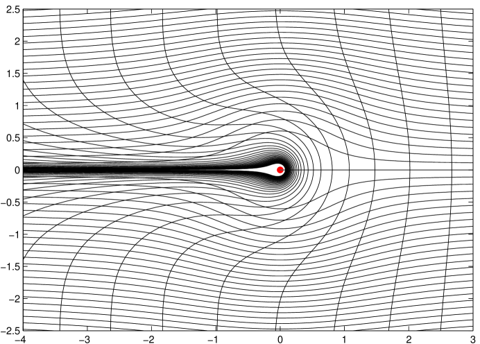
Figure 2. The result of the incompressible flow from $t=-\infty$ to $t=0$ with $n=2$, momentum concentrated at one point and $K=K_{0,\eta}$, $\eta=1$.

Now consider the case of two landmark points $P_{1},P_{2}$ with momenta $m_{1},m_{2}$. By conservation of total momentum, $m_{1}+m_{2}$ is a constant. We can reduce this Hamiltonian system by fixing the total momentum $\overline{m}$ and dividing by translations. We get a new system in the variables $\delta P=P_{2}-P_{1}$ and $\delta m=m_{2}-m_{1}$ with equations of motion:

$$E =\kappa\cdot\left(|\delta m|^{2}+|\overline{m}|^{2}\right)+\sum_{ij}K_{ij}(\delta P)\cdot\left(\overline{m}_{i}\overline{m}_{j}-\delta m_{i}\delta m_{j}\right)$$

$$\frac{d(\delta P_{i})}{dt} =\kappa\cdot\delta m_{i}-\sum_{j}K_{ij}(\delta P)\cdot\delta m_{j}$$

$$\frac{d(\delta m_{i})}{dt} =-\sum_{jk}\partial_{x_{i}}K_{jk}(\delta P)\cdot(\overline{m}_{j}\overline{m}_{k}-\delta m_{j}\delta m_{k})$$

or, letting $\delta P=\rho\cdot u$ for a unit vector $u$, in geometric form:

$$E =\kappa\cdot\left(|\delta m|^{2}+|\overline{m}|^{2}\right)+K_{1}(\rho)\left(|P_{u}\overline{m}|^{2}-|P_{u}\delta m|^{2}\right)$$

$$\qquad+K_{2}(\rho)\left(|P_{u^{\perp}}\overline{m}|^{2}-|P_{u^{\perp}}\delta m|^{2}\right)$$

$$\frac{d(\delta P)}{dt} =\kappa\cdot\delta m-K_{1}(\rho)\cdot P_{u}\delta m-K_{2}(\rho)\cdot P_{u^{\perp}}\delta m$$

$$\frac{d(\delta m)}{dt} =-\left(K_{1}^{\prime}(\rho)(|P_{u}\overline{m}|^{2}-|P_{u}\delta m|^{2})+K_{2}^{\prime}(\rho)(|P_{u^{\perp}}\overline{m}|^{2}-|P_{u^{\perp}}\delta m|^{2}\right)u$$

$$\qquad-\frac{K_{1}(\rho)-K_{2}(\rho)}{\rho}\left(\langle\overline{m},u\rangle P_{u^{\perp}}\overline{m}-\langle\delta m,u\rangle P_{u^{\perp}}\delta m\right)$$

Note that the derivatives of $\delta p$ and $\delta m$ lie in the span of $\delta P,\delta m$ and $\overline{m}$. Thus this three dimensional space is constant in time so we can assume $\delta P,\delta m,\overline{m}\in\mathbb{R}^{3}$. The total angular momentum is:

$$\omega=P_{1}\wedge m_{1}+P_{2}\wedge m_{2}=\tfrac{P_{1}+P_{2}}{2}\wedge\overline{m}+\tfrac{1}{2}\delta P\wedge\delta m.$$

If $\overline{m}=0$, then the two vectors $\delta p,\delta m$ always lie in a fixed two dimensional space and their cross product is constant, equal to $2\omega$. We can then make a further symplectic reduction and compute what happens in terms of the three scalar variables $\rho,\langle\delta P,\delta m\rangle,|\delta m|$ which moreover must lie on one sheet of a hyperboloid:

$$4|\omega|^{2}+\langle\delta P,\delta m\rangle^{2}=\rho^{2}\cdot|\delta m|^{2},\quad\rho\cdot|\delta m|\geq 2|\omega|.$$

The energy then simplifies to

$$E =(\kappa-K_{2}(\rho))|\delta m|^{2}-\tfrac{K_{1}(\rho)-K_{2}(\rho)}{\rho^{2}}\langle\delta P,\delta m\rangle^{2}$$

$$=\tfrac{\kappa-K_{1}(\rho)}{\rho^{2}}\langle\delta P,\delta m\rangle^{2}+4\tfrac{\kappa-K_{2}(\rho)}{\rho^{2}}|\omega|^{2}.$$

Its level curves on the hyperboloid must then be the geodesics. Note that as long as the kernel is $C^{2}$, $(\kappa-K_{1}(\rho))/\rho^{2}$ and $(K_{1}(\rho)-K_{2}(\rho))/\rho^{2}$ are finite at the origin hence bounded.

We can illustrate this in the simple case of 3-space with kernel $K_{0,1},p=3$. As stated above, then the smoothing kernel is $C^{2}$ and has the elementary expression

$$G^{(3)}_{1}(x)=(1+|x|)e^{-|x|}=1-\tfrac{|x|^{2}}{2}+\cdots.$$

It’s easy to calculate the mean of this function over a ball and we get:

$$\text{Mean}_{B_{|x|}}\left(G^{(3)}_{1}\right)(x) =24|x|^{-3}\left(1-e^{-|x|}\left(1+|x|+\tfrac{|x|^{2}}{2}+\tfrac{|x|^{3}}{8}\right)\right)$$

$$=e^{-|x|}\left(1+\sum_{n=4}^{\infty}\tfrac{4}{n!}|x|^{n-3}\right)$$

$$=1-\tfrac{3|x|^{2}}{10}+\cdots$$

hence

$$\kappa=\tfrac{2}{3},\quad K_{1}=\tfrac{2}{3}-\tfrac{1}{5}x^{2}+\cdots,\quad K_{2}=\tfrac{2}{3}-\tfrac{2}{5}x^{2}+\cdots.$$

A typical plot of the contours of $E$ in the $(\rho,|\delta m|)$-plane is shown in Figure 3.

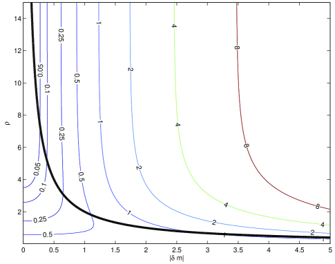
Figure 3. Level sets of energy for the collision of two vortons with $\overline{m}=0$, $\eta=1$, $\omega=1$. The coordinates are $\rho=|\delta P|$ and $|\delta m|$, and the state space is the double cover of the area above and right of the heavy black line, the two sheets being distinguished by the sign of $\langle\delta m,\delta P\rangle$. The heavy black line which is the curve $\rho\cdot|\delta m|=\omega$ where $\langle\delta m,\delta P\rangle=0$. Each level set is a geodesic. If they hit the black line, they flip to the other sheet and retrace their path. Otherwise $\rho$ goes to zero at one end of the geodesic.

In the figure, if an orbit hits the heavy black line defined by $\rho\cdot|\delta m|=\omega$, then $\langle\delta P,\delta m\rangle$ is instantaneously zero and, along its orbit, changes sign. On the two-sheeted cover given by including this sign, this is a smooth orbit in which $\rho$ decreases to a minimum where $\langle\delta P,\delta m\rangle=0$ and then increases. One sees that there are two types of orbits: scattering orbits where the vortons separate infinitely at both $t=\pm\infty$ and $\rho$ has a minimum at some point in time; and capturing orbits which either start or end at infinity but spiral indefinitely, getting closer and closer, at the other limit. Which happens depends on the relative size of the angular momentum and the energy exactly as in the simpler case studied in [12]. Here if $E\geq(8/5)|\omega|^{2}$, the points attract while if $E<(8/5)|\omega|^{2}$, they scatter.

When the landmark points attract, this simple system forms higher order singularities. If we take coordinates so that $\delta P$ is on the $x_{1}$-axis and $\delta m$ in the $(x_{1},x_{2})$-plane, then for $\rho$ very small, we have:

$$P_{1}=(\rho/2,0,0),\quad P_{2}=(-\rho/2,0,0),\quad m_{1}=\frac{1}{\rho}(C,\omega,0),\quad m_{2}=-\frac{1}{\rho}(C,\omega,0)$$

where $2C=\langle\delta P,\delta m\rangle$, hence (using the limiting values of the $k$-terms in the formula for energy) we get $C^{2}\approx\tfrac{5}{4}E-2\omega^{2}>0$. Then, as these points approach each other, the corresponding global vector field in $\mathbb{R}^{3}$ approaches:

$$v_{i}(x) =-\frac{(K_{0,1})_{i\cdot}(x+(\rho/2,0,0))-(K_{0,1})_{i\cdot}(x-(\rho/2,0,0))}{\rho}\cdot\left(\begin{array}[]{cc}C\\ \omega\end{array}\right)$$

$$\approx-\partial_{x_{1}}\left((K_{0,1})_{i1}\cdot C+(K_{0,1})_{i2}\cdot\omega\right)$$

This vector field for $\omega=2C$ is illustrated in Figure 4. Whereas for any column vector $A$, $K_{01}\cdot A$ is a vortex ring with maximum norm at the origin and maximum vorticity along a ring centered at the origin and lying in a plane perpendicular to $A$, its derivative $v$ is now zero at the origin and it has maximum vorticity there. In our case, computing the derivatives $Dv(0)$, we find that near the origin, the flowlines of $v$ spiral in along the $(x_{1},x_{2})$-plane and shoot out along the $x_{3}$-axis.

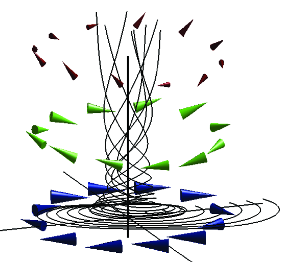
Figure 4. Streamlines and MatLab’s ‘coneplot’ to visualize the vector field given by the $x_{1}$-derivative of the kernel $K_{0,1}$ times the vector $(1,2,0)$. See text.

Another case which is easy to explore is when $\overline{m}$ lies in the plane spanned by $\delta P$ and $\delta m$. The angular momentum no longer descends to a function on the $\delta P,\delta m$ space but we may numerically integrate the geodesic equations. Figure 5 shows geodesics all starting with the same $\delta P$ and $\delta m$ but with varying $\overline{m}$ fixed along the $y$-axis.

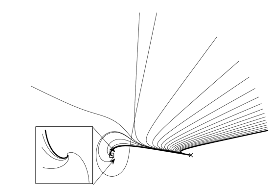
Figure 5. Geodesics in the $\delta P$ plane all starting at the point marked by an X but with $\overline{m}$ along the $y$-axis varying from 0 to 10. Here $\eta=1$, the initial point is $(5,0)$ and the initial momentum is $(-3,.5)$. Note how the two vortons repel each other on some geodesics and attract on others. A blow up shows the spiraling behavior as they collapse towards each other.

It is extremely easy to compute landmark geodesics numerically even in much more complex situations and we hope that, letting $\eta\rightarrow 0$, this may be a useful tool to exploring the instabilities of Euler’s equation itself.

References

[1]Handbook of mathematical functions with formulas, graphs, and mathematical tables.Edited by Milton Abramowitz and Irene A. Stegun.
Reprint of the 1972 edition. Dover Publications, Inc., New York, 1992
[2]V.I. Arnold.
Sur la géometrie différentielle des groupes de Lie de
dimension infinie et ses applications à l’hydrodynamique des
fluides parfaits.
Ann. Inst. Fourier 16 (1966), 319–361.
[3]M. Bauer, P. Harms, and P. W. Michor.
Almost local metrics on shape space of hypersurfaces in n-space,
SIAM J. Imaging Sci. 5 (2012), 244-310.
[4]Thomas Buttke.
The fast adaptive vortex method.
J. Comput. Phys. 93 (1991), 485.
[5]Roberto Camassa and Darryl Holm.
An Integrable shallow water equation with peaked solutions.
Physical Review Letters, 71 (1993), 1661-1664.
[6]Alexandre Chorin.
Vorticity and Turbulence.Springer-Verlag, (1994).
[7]Ricardo Cortez.
On the accuracy of impulse methods for fluid flow.
SIAM J. Sci. Comput. 19 (1998), 1290 1302
[8]Darryl Holm, Jerry Marsden and Tudor Ratiu.
The Euler-Poincarè equations and Semidirect Products with Applications to Continuum Theories.
Advances in Math., 137 (1998), 1-81.
[9]Darryl Holm and Jerry Marsden.
Momentum maps and measure-valued solutions for the EPDiff equation.
in The Breadth of Symplectic and Poisson geometry, A festschrift for Alan Weinstein,
Progress in Mathematics, 232 (2004), 203-235.
[10]Lars Hörmander,
The analysis of linear partial differential operators. I,
Springer-Verlag, Berlin, 1983,
[11]Tosio Kato.
Quasi-linear equations of evolution, with applications to partial differential equations,
in Springer Lecture Notes in Math, 448 (1975), 27-50.
[12]Mario Micheli, Peter Michor, David Mumford.
Sectional curvature in terms of the cometric, with applications to the Riemannian manifolds of landmarks.
SIAM Journal on Imaging Sciences. 5 (2012), 394-433.
arXiv:1009.2637
[13]Mario Micheli, Peter W. Michor, David Mumford.
Sobolev Metrics on Diffeomorphism Groups and the Derived Geometry of Spaces of Submanifolds.
Izvestiya: Mathematics 77:3 (2013), 541-570.
arXiv:1202.3677
[14]Peter Michor, David Mumford.
Vanishing geodesic distance on spaces of submanifolds and diffeomorphisms.
Documenta Mathematica, 10 (2005), 217–245.
[15]Peter W. Michor and David Mumford.
An overview of the Riemannian metrics on spaces of curves using the Hamiltonian approach.
Applied and Computational Harmonic Analysis 23 (2007), 74-113.
arXiv:math.DG/0605009
[16]Peter W. Michor and David Mumford.
A zoo of diffeomorphism groups on .
Annals of Global Ananlysis and Geometry, (2013).
doi:10.1007/s10455-013-9380-2.
[17]Michael I. Miller , Gary E. Christensen , Yali Amit and Ulf Grenander.
Mathematical Textbook Of Deformable Neuroanatomies
Proceedings National Academy of Science 90 (1993), 11944-11948.
[18]Michael Miller, Alain Trouvé and Laurent Younes.
On the Metrics and Euler-Lagrange equations of Computational Anatomy.
Annual Review of Biomedical Engineering (2002), 375-405.
[19]V. I. Oseledets.
On a new way of writing the Navier-Stokes equations: The Hamiltonian formalism.
Communications of the Moscow Mathematical Society (1988).
Translation in Russian Mathematics Surveys, 44 (1989), 210-211.
[20]P. H. Roberts.
A Hamiltonian theory for weakly interacting vortices.
Mathematika 19 (1972), 169-179.