RB Drift Momentum Spectrometer
Abstract
We propose a new type of momentum spectrometer, which uses the RB drift effect to disperse the charged particles in a uniformly curved magnetic field. This kind of RB spectrometer is designed for the momentum analyses of the decay electrons and protons in the PERC (Proton and Electron Radiation Channel) beam station, which provides a strong magnetic field to guide the charged particles in the instrument. Instead of eliminating the guiding field, the RB spectrometer evolves the field gradually to the analysing field, and the charged particles can be adiabatically transported during the dispersion and detection. The drifts of the particles have similar properties as their dispersion in the normal magnetic spectrometer. Besides, the RB spectrometer is especially ideal for the measurements of particles with low momenta and relative large incident angles. We present a design of the RB spectrometer, which can be used in PERC. The resolution of the momentum spectra can reach 14.4 keV/c, if the particle position measurements have a resolution of 1 mm.
keywords:
momentum spectrometer , RB drift effect , PERC , magnetic field , adiabatic transport , neutron decay1 Introduction
The beam station PERC (Proton and Electron Radiation Channel) [1], for the experiments of free neutron decay, is under development [2]. The motivation of PERC is to supply an intense beam of well defined electrons and protons () from free neutron decay. With the general-purpose -beam, various quantities related to the physics in and beyond the Standard Model can be measured [3, 4, 5, 6, 7].
PERC provides in the instrument a neutron decay volume, where the free neutrons are imported and decay into charged electrons, protons, and neutral electron anti-neutrinos. With a series of coils, a specified static magnetic field is applied in the instrument. The charged decay spiral along the magnetic field lines, and are guided from the decay to the detection area. Fig. 1 sketches the principle of PERC.
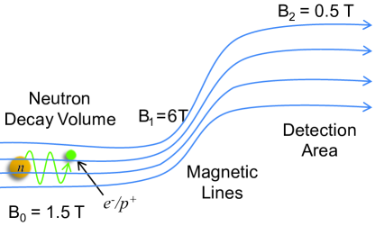
The neutron decay volume has a magnetic field of = 1.5 T. After the decay volume, a magnetic field barrier = 6 T is applied. The particles propagate adiabatically in PERC, hence the pitch angles of them, i.e., the angles between the particle momentum and the magnetic field , fulfil
| (1) |
Therefore, only the with pitch angles at smaller than the critical angle can pass through the field barrier
| (2) |
After the barrier, the guiding field is gradually decreased to = 0.5 T at the detection area, where the particles can be processed and measured.
As for the measurements of the particles, the loss free energy spectroscopy for electrons has been demonstrated in [8, 9]. While in the experiments with PERC, a spectrometer for the momentum measurements besides the energy sensitive detector is desired. The principle of a normal magnetic spectrometer after PERC is sketched in Fig. 2.
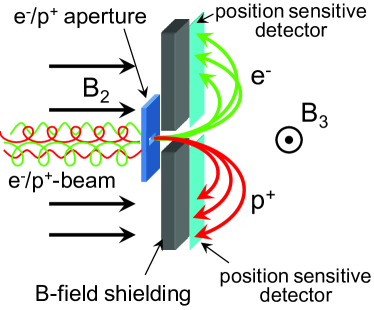
At the end of PERC, the magnetic spectrometer must firstly shield the guiding field , and apply a vertical analysing magnetic field . The incident from PERC pass through a small aperture, then disperse in the field. The position sensitive detectors for electrons and protons are placed on both sides of the incident window. The dispersion distance of a particle in the spectrometer is then
| (3) |
where and are the momentum and charge of the particle, is its incident angle according to the normal of the detector plane.
Compared with the energy resolving detectors, the magnetic spectrometer is versatile, that it can realize various measurements in PERC [1], also detect the electrons and protons at the same time. Technically, the position sensitive detectors highly suppress the backscattering problem of and the background. The momentum spectrum of the decay electrons has higher resolution in the low energy scale, thus is especially needed for the estimation of the Fierz interference term in neutron decay [3].
However, because of the strong magnetic guiding field of PERC, we found difficulties in the design of the magnetic spectrometer. The spectrometer has to drastically decrease the guiding field to zero at the incident window, whereas the magnetic lines do not vanish, but spread in vertical directions. When the pass the vertical field, the pitch angles of them are highly distorted either in adiabatic or in non-adiabatic transports, as shown in Fig. 3.
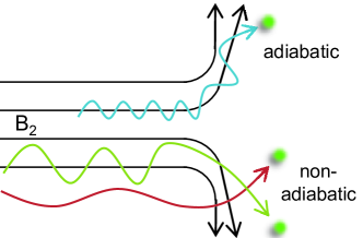
The distortion of the pitch angles strongly depends on the field distribution and the momenta, thus are not predictable nor controllable [10]. Therefore, the distribution of the particles in the spectrometer can hardly represent their momenta.
In this case, we propose a method of RB drift momentum spectrometer, which can realize the momentum analyses of the without eliminating the guiding field of PERC.
2 Principle of the RB drift momentum spectrometer
When a charged particle propagates in a curved magnetic field, it has the drift effect perpendicular to the magnetic field and the field curvature , so called as the RB drift. The drift velocity of the first order can be expressed as [11]
| (4) |
where is the mass of the particle, and are the velocity components parallel and vertical to the magnetic field line. In a static magnetic field, the velocity components can be expressed with the absolute velocity and the pitch angle
| (5) |
Suppose that we apply a uniformly curved magnetic field, with the curvature and the field strength as constants, then the curved magnetic field lines are distributed parallelly and coaxially, as shown in Fig. 4.
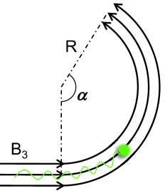
According to Eq. 4, the drift velocity is a constant in the uniformly curved magnetic field, and the higher order contributions induced by are zero [12, 13, 14]. During a propagating time of , the drift distance of a particle is
| (6) |
where is the bending angle of the route of the particle gyration center during the time
| (7) |
as marked in Fig. 4. is a factor related to the particle pitch angle
| (8) |
Compare Eq. 6 with Eq. 3, the behaviour of the RB drift is similar as that of the particle dispersion in the magnetic spectrometer. The drifts or the dispersion distances in both cases are proportional to the particle momentum, and inversely proportional to the analysing magnetic field and the particle charge.
With this principle, we propose a design of the RB drift momentum spectrometer, as shown in Fig. 5.
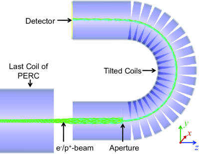
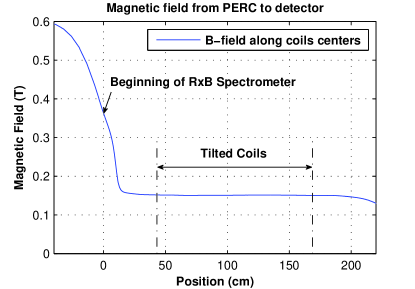
At the beginning of the RB spectrometer, we apply several connected coils to gradually decrease the guiding field of PERC from 0.5 T to 0.15 T, with the field gradient satisfies the adiabatic condition of transports. After that, a series of tilted coils generates a 180∘ bended magnetic field. Along the central line of the tilted coils, the curvature of magnetic field line is = 40 cm, and the field strength is kept as = 0.15 T. Fig. 6 plots the magnetic field from the end of PERC to the RB spectrometer detector.
At the beginning of the tilted coils, we apply an aperture of 11 cm2 to define the size of the incident -beam. The particles through the aperture follow the curved magnetic lines, and turn 180∘ then reach the detector on top. During the propagation, they drift along the -axis according to their charges and momenta.
Hence the RB drift spectrometer, instead of eliminating the guiding field of PERC, evolves the field smoothly and gradually to the analysing magnetic field. The particles can be transported adiabatically during the processes, and their angular information can be kept and measured.
Table 1 lists the parameters of the standard configuration of the RB spectrometer design.
| Parameter | Comment | Value |
|---|---|---|
| Analysing field | 0.15 T | |
| Field line curvature | 40 cm | |
| Aperture width | 1 cm | |
| Aperture height | 1 cm | |
| Bending angle | ||
| Max. pitch angle | 9.1∘ | |
| Max. gyration radius | 0.42 cm | |
| Max. drift | 8.29 cm |
and in Table 1 are the width and height of the aperture along the - and -axes. and are the maximum pitch angle and gyration radius of the decay in the field
| (9) |
where = 1.19 MeV/c is the maximum momentum of from the free neutron decay [15].
With the standard configuration, the maximum drift for is 8.29 cm.
3 Corrections on RB drift spectrometer
In the RB spectrometer, the particle distribution on the detector is influenced by the properties of the particles and the instrument.
3.1 pitch angle
Compare Eq. 8 with Eq. 3, the influence of the correction factor induced by the incident angle of particles in the RB spectrometer is much smaller than that in the magnetic spectrometer. In Fig. 7, the magnitudes of both correction factors are plotted.
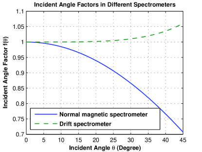
For 10∘, the in the RB drift is negligible as less than 10-4 deviated from 1, while the deviation in the magnetic spectrometer is 1.510-2. Hence the RB spectrometer has large acceptance of incident angles, which is a significant advantage.
3.2 Gyration radius and aperture width
In the RB spectrometer, the gyration radii of the particles remain during the drifts and the detection. For a given momentum, the maximum gyration radius of the particles is
| (10) |
Through the aperture, the size of the -beam on the detector will be
| (11) |
as sketched in Fig. 8 (a). Therefore, the maximum deviation induced by the gyration radius relative to the drift is
| (12) |
3.3 Beam height and curvature
In the curved magnetic field, the field strength has a gradient along
| (13) |
and are the field strength and the curvature along the central line of the tilted coils. The particles at different positions along will experience deviated magnetic fields, thus have the drift
| (14) |
where is the vertical position of the particle on the detector relative to the beam center. The maximum deviation of the drift is
| (15) |
Hence the -beam height relative to the field curvature tilts the particle distribution on the detector, as sketched in Fig. 8 (b). For a detector only sensitive to the -position, the measured particle distribution is widened.
3.4 Particle distribution on detector
The dispersion of the particles in the drift spectrometer is mainly influenced by the systematics of , , and . Fig. 8 shows the sketchy distribution of electrons on the detector affected by these factors.
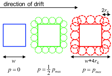
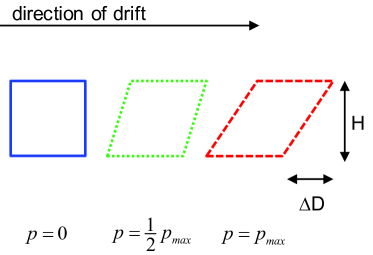
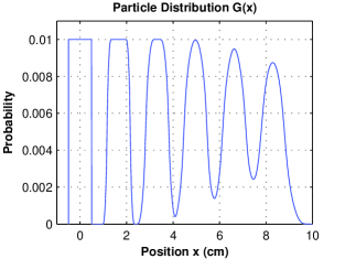
Fig. 9 shows the simulated distributions of electrons on the detector, with discrete momenta from 0 to 1.19 MeV/c.
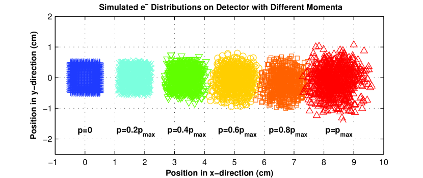
The deviation of the drift caused by is a constant, while that induced by and are proportional to the drift distance. Hence at the low momentum range, the RB spectrometer has better performance.
Furthermore, in normal magnetic spectrometer, the particles with cannot be totally measured if their dispersion distances are smaller than the aperture width . While as shown in Fig. 9, the RB spectrometer can measure the full range of the momentum.
4 Transfer function
The motions of the particles in the RB spectrometer are clearly defined during the drift processes. The transfer function, i.e., the relation between the momentum spectrum and the particle distribution on the detector , can be calculated and used in the data analyses. In this section, we discuss the transfer function including the corrections of , , and . The incident angle correction and the higher order contributions, e.g., the deviation induced by , the deviation induced by the gradient along , are not considered here.
4.1 Particle distribution from point source
We assume the from the decay volume of PERC are homogeneously distributed in the open window of the aperture. If the aperture is sufficiently thin, it does not distort the angular distribution of the particles. In addition, the size of the -beam in front of the aperture is much larger than that of the aperture. Therefore, the particles that pass through the aperture, can be treated as emitted from the aperture’s open window.
For the particles emitted from a point source at position with given momentum and pitch angle, their distribution along the -axis is given as [16]
| (16) |
where denotes the complete elliptical integral of the first kind.
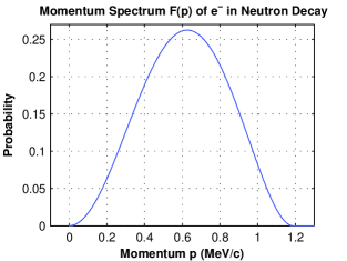
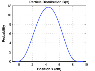
4.2 Angular distribution of particles in field
If we apply unpolarized neutrons in PERC experiments, the are isotropically emitted in the decay volume [3]. Their angular distribution in the field is
| (17) |
With Eq. 1, when the particles propagate from to , their angular distribution is
| (18) |
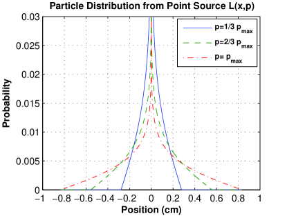
We integrate Eq. 16 over , the particle distribution along the -axis from a point source is then
| (19) |
Fig. 10 plots the distribution of particles in the field with different momenta.
4.3 Transmission function of aperture
Since the distance from the aperture to the detector is much longer than the helical pitches of the particles, we assume the particle distribution on the detector from any point in the aperture follows Eq. 19.
Define the transmission function of the aperture along the -axis as
| (20) |
On the detector, the particles from the open window of the aperture then have a distribution of
| (21) |
which is the convolution of the aperture function and the distribution of point source.
4.4 Correction of
For the correction of beam height , we consider the particle distribution along the -axis. For simplicity, we use the condition = , so the distribution along the -axis is the same as Eq. 21, i.e., . Since the factor tilts the particle distribution on detector, is projected on the -axis. According to Eq. 14, the projection can be written as
| (22) |
4.5 Transfer function
All together, we take the corrections related to , , , as well as the drift into account. The total transfer function is then the convolution of the distributions in Eq. 21 and Eq. 22
| (23) |
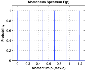
For a given momentum spectrum , the particle distribution on the detector can be derived
| (24) |
In experiments, can be measured by position sensitive detectors. To evaluate from Eq. 24, which is the Fredholm integral equation of first type, a numerical method is to convert the integral into the quadrature calculation, the and into arrays, thus convert the kernel function into a square matrix [17, 18]. The transfer function then can be written as
| (25) |
and the momentum spectrum can be evaluated
| (26) |
In this case, the and have the same number of rows, thus the same resolution. In the standard configuration, if has a resolution of 1 mm, the momentum spectrum can reach a resolution of 14.4 keV/c.
5 Conclusion
The RB drift spectrometer offers the opportunity of momentum measurements of charged particles in the instrument with guiding fields, in which case the normal magnetic spectrometers cannot work well. In this proposed drift spectrometer, the guiding field is not eliminated, but gradually evolved to the analysing field. The drifts of the particles in the uniformly curved magnetic field have similar behaviours as in the normal magnetic spectrometer.
As a conclusion, the RB spectrometer has the advantages:
-
1.
Adiabatic transports of particles. As shown in Fig. 6, from the guiding field to the detector of the RB spectrometer, the charged particles can be adiabatically transported. The angular distribution of the particles can be kept and measured.
-
2.
Low momentum measurements. As shown in Fig. 9, the particles with very small momentum can be measured in the RB spectrometer, while they cannot be measured in normal magnetic spectrometer if their dispersion .
-
3.
Large acceptance of incident angle. As shown in Fig. 7, the direct correction induced by the incident angle is very small as less than 10-4 when 10∘.
As a conceptual design of RB spectrometer, the particle drifts are considerably influenced by the systematics related to both the instrument and the particle properties. Table 2 lists the maximum sizes of the corrections in the standard configuration.
| Correction | Comment | Max. Size |
|---|---|---|
| 4 | Gyration Radius | 2.010-1 |
| Aperture Width | 1.210-1 | |
| Aperture Height | 6.710-2 | |
| Field Homogeneity | 810-3 | |
| Incident Angle | 810-5 |
However, the motions of the particles are clearly defined during the drifts, thus the transfer function of the particles can be well known. Experimentally, one is able to fit the momentum spectrum to the measured particle distribution , or numerically evaluate from . In the standard configuration, if the position detector has a resolution of 1 mm, the momentum spectra can reach a resolution of 14.4 keV/c. Additionally, by performing detector calibration with defined particle sources, the systematic errors can be controlled at low level.
Besides, there is also room for improvement of the RB spectrometer design. For further development, we can decrease the corrections, e.g., by optimizing the bending angle , the curvature , and the analysing magnetic field . The transfer function in this article only considers the motions of the particles to the first order. The higher order contributions, e.g., the acceleration , the deviation of curvature induced by the drift , are more complicated [13, 14]. To obtain the transfer function with high accuracies, we can apply fine simulations of trajectories in the RB spectrometer.
6 Acknowledgement
We would like to thank MSc. Z. Lee (Electron Microscopy Group of Materials Science, Ulm University) for helpful discussions about the transfer function. This work is supported by the German Research Foundation as part of the Priority Program 1491, and the Austrian Science Fund under contracts No. I 528-N20 and I 534-N20.
References
- Dubbers et al. [2008] D. Dubbers, H. Abele, S. Baeßler, B. Märkisch, M. Schumann, T. Soldner, O. Zimmer, Nucl. Instr. and Meth. A 596 (2008) 238–247.
- Konrad et al. [2012] G. Konrad, H. Abele, M. Beck, C. Drescher, D. Dubbers, J. Erhart, H. Fillunger, C. Gösselsberger, W. Heil, M. Horvath, E. Jericha, C. Klauser, J. Klenke, B. Märkisch, R. K. Maix, H. Mest, S. Nowak, N. Rebrova, C. Roick, C. Sauerzopf, U. Schmidt, T. Soldner, X. Wang, O. Zimmer, T. P. collaboration, Journal of Physics: Conference Series 340 (2012) 012048.
- Jackson et al. [1957] J. D. Jackson, S. B. Treiman, H. W. Wyld, Phys. Rev. 106 (1957) 517–521.
- Herczeg [2001] P. Herczeg, Prog. Part. Nucl. Phys. 46 (2001) 413–457.
- Severijns et al. [2006] N. Severijns, M. Beck, O. Naviliat-Cuncic, Rev. Mod. Phys. 78 (2006) 991–1040.
- Abele [2008] H. Abele, Prog. Part. Nucl. Phys. 60 (2008) 1–81.
- Dubbers and Schmidt [2011] D. Dubbers, M. G. Schmidt, Rev. Mod. Phys. 83 (2011) 1111–1171.
- Bopp et al. [1986] P. Bopp, D. Dubbers, L. Hornig, E. Klemt, J. Last, H. Schütze, S. J. Freedman, O. Schärpf, Phys. Rev. Lett. 56 (1986) 919–922.
- Abele et al. [1993] H. Abele, G. Helm, U. Kania, C. Schmidt, J. Last, D. Dubbers, Physics Letters B 316 (1993) 26 – 31.
- Varma [1971] R. K. Varma, Phys. Rev. Lett. 26 (1971) 417–420.
- Dinklage [2005] A. Dinklage, Plasma Physics: Confinement, Transport And Collective Effects, Lecture Notes in Physics, Springer, 2005.
- Eržen et al. [2009] D. Eržen, J. P. Verboncoeur, J. Duhovnik, N. Jelić, Eur. Phys. J. D 54 (2009) 409–415.
- Kruskal [1962] M. Kruskal, Journal of Mathematical Physics 3 (1962) 806–828.
- Littlejohn [1983] R. G. Littlejohn, Journal of Plasma Physics 29 (1983) 111–125.
- Nakamura, K. et al. (2010) [Particle Data Group] Nakamura, K. et al. (Particle Data Group), J. Phys. G: Nucl. Part. Phys. 37.7A (2010) 075021.
- Dubbers et al. [2008] D. Dubbers, B. Maerkisch, F. Friedl, H. Abele (2008).
- Delves and Mohamed [1988] L. Delves, J. Mohamed, Computational Methods for Integral Equations, Cambridge University Press, 1988.
- Press [2007] W. Press, Numerical Recipes: The Art of Scientific Computing, Cambridge University Press, 2007.