Theory of spin-orbit enhanced electric-field control of magnetism in multiferroic BiFeO₃

Abstract

We present a microscopic theory that shows the importance of spin-orbit coupling in perovskite compounds with heavy ions. In BiFeO₃ (BFO) the spin-orbit coupling at the bismuth ion sites results in a special kind of magnetic anisotropy that is linear in the applied $E$-field. This interaction can convert the cycloid ground state into a homogeneous antiferromagnet, with a weak ferromagnetic moment whose orientation can be controlled by the $E$-field direction. Remarkably, the $E$-field control of magnetism occurs without poling the ferroelectric moment, providing a pathway for reduced energy dissipation in spin-based devices made of insulators.

The ability to control magnetism using electric fields is of great fundamental and practical interest. It may allow the development of ideal magnetic memories with electric write and magnetic read capabilities scott07 . The traditional mechanism of $E$-field control of magnetism is based on the dependence of magnetic anisotropy on the filling of $d$-orbitals. This allows $E$-field control of magnetism in metallic materials such as magnetic semiconductors chiba08 and ferromagnetic thin films shiota12 , but not in insulators. A method to influence magnetism using $E$-fields in insulators is desirable because it would not generate electric currents, potentially allowing the design of spin-based devices with much lower energy dissipation rovillain10 .

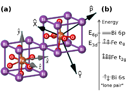
Figure 1: (color online) (a) Conventional unit cell for BFO. The simple cubic axes $\bm{\hat{x}}$, $\bm{\hat{y}}$, $\bm{\hat{z}}$ are denoted by grey vectors. The ferroelectric polarization $\bm{P}$ is shown pointing along [111], arising mostly from the displacement of Bi ions with respect to the oxygens. The directions $\bm{\hat{X}}$ and $\bm{\hat{Y}}$ denoted by black vectors describe the plane perpendicular to $\bm{P}$ noteaxes . (b) Energy level diagram for Fe${}^{3+}=[{\rm Ar}]3d^{5}$ and Bi${}^{3+}=[{\rm Pt}]6s^{2}$ orbitals in BFO; the Fermi level lies between $E_{3d}$ and $E_{6p}$.

In insulators, the interactions that couple spin to electric degrees of freedom, the so called magnetoelectric interactions, are usually too weak to induce qualitative changes to magnetic states. A remarkable exception occurs in the presence of the linear magnetoelectric effect (LME), an interaction that couples spin and charge linearly in either the external electric field $\bm{E}$ or the internal electric polarization $\bm{P}$ of the material. Multiferroic insulators with coexisting magnetic and ferroelectric phases have emerged as the natural physical system to search for LME and enhanced cross correlation between electricity and magnetism spaldin10 . In a large class of multiferroic materials, the dominant form of LME was found to be due to the spin-current effect (a type of Dzyaloshinskii-Moriya interaction katsura05 ), that couples localized spins according to ${\cal H}_{{\rm SC}}=\sum_{i<j}J_{{\rm SC}}(\bm{P}\times\bm{R}_{ij})\cdot(\bm{S}_{i}\times\bm{S}_{j})$, with $\bm{R}_{ij}$ the vector linking the atomic location of spin $\bm{S}_{i}$ to the atomic location of spin $\bm{S}_{j}$. In manganese-based multiferroics, the spin-current interaction leads to magnetic induced ferroelectricity and thus allows magnetic field control of ferroelectricity kimura03 .

For $E$-field control of magnetism, research has been centered instead on iron-based multiferroics, with bismuth ferrite [BiFeO₃ or BFO] being the most notable example catalan09 . At temperatures below $1143$ K, BFO develops a strong electric polarization $P=100$ $\mu$C/cm² that points along one of the eight cube diagonals of its unit cell [Fig. 1(a)]. It becomes an antiferromagnet below $643$ K with Fe spins forming a spiral of the cycloid type, described by antiferromagnetic Néel vector $\bm{\hat{L}}=\sin{(\bm{q}\cdot\bm{r})}\bm{\hat{q}}+\cos{(\bm{q}\cdot\bm{r})}\bm{\hat{P}}$. The microscopic origin of the cycloid can also be understood as arising from the spin-current interaction rahmedov12 . Plugging the cycloid $\bm{L}$ into ${\cal H}_{{\rm SC}}$, one finds that the lowest energy state is always achieved when the cycloid wavevector $\bm{q}$ is perpendicular to $\bm{P}$. Hence the spins are pinned to the plane formed by $\bm{P}$ and $\bm{q}$. This fact has been central to all demonstrations of $E$-field control of magnetism in multiferroics published to date; the application of an $E$-field poles $\bm{P}$ from one cube diagonal to another, forcing the spin cycloidal arrangement to move into a different plane lebeugle08 ; heron11 .

In addition, BFO is known to have a weak magnetization $\bm{M}\propto\bm{\hat{Z}}\times\bm{L}$ that is generated by an additional Dzyaloshinskii-Moriya interaction ederer05 ; desousa09 (with $\hat{\bm{Z}}\parallel\hat{\bm{P}}$). When $\bm{L}$ is in a cycloidal state, $\bm{M}$ is sinusoidal and averages out to zero over distances larger than the cycloid wavelength. The amplitude of the oscillatory $|M|=0.06\mu_{B}/{\rm Fe}$ was measured recently ramazanoglu11b . Therefore, a method to convert the cycloid into a homogeneous state would preclude $\bm{M}$ from averaging out to zero, with potential applications to electrically-written magnetic memories.

A recent experiment rovillain10 suggested that the spin-current interaction is not the only LME present in BFO. The application of an external $E$-field to bulk BFO was shown to result in a giant shift of magnon frequencies that was linear in $\bm{E}$ and $10^{5}$ times larger than any other known $E$-field effect on magnon spectra.

In this letter, we present a microscopic theory of $E$-field induced magnetic anisotropy, and argue that it can provide an effective source of LME in insulators with large spin-orbit coupling. Our predicted LME explains the origin of the $E$-field effect on magnon spectra measured in bulk BFO rovillain10 . Moreover, we show that this effect is capable of switching the cycloidal spin state of BFO into a homogeneous magnetic state with its orientation tunable by the direction of the applied $E$-field.

Model and microscopic calculation of LME.—Our microscopic Hamiltonian for coupling between spin and electric-field has three contributions, ${\cal H}={\cal H}_{{\rm latt}}+{\cal H}_{{\rm elec}}+{\cal H}_{{\rm SO}}$. The first term is due to the lattice, ${\cal H}_{{\rm latt}}=-\hbar^{2}\nabla^{2}/(2m_{e})+V_{{\rm crystal}}(\bm{r})$, with $m_{e}$ and $\bm{r}$ the free electron mass and its coordinate, respectively. The second term is called “electronic”, ${\cal H}_{{\rm elec}}=-e\bm{r}\cdot\bm{E}$, with $e<0$ the electron’s charge. The last and most important term is the spin-orbit interaction, ${\cal H}_{{\rm SO}}=\zeta\bm{\ell}\cdot\bm{\sigma}$, with $\bm{\ell}=-i\bm{r}\times\bm{\nabla}$ the electron’s orbital angular momentum and $\bm{\sigma}/2$ its spin operator. We take the spin-orbit interaction to be dominated by the heaviest ion of the lattice, and take bismuth in BFO as a prototypical example.

Single ion anisotropy is known to arise as a correction to the total spin energy that is second order in the spin-orbit interaction abragam70 . In our case the largest contribution arises in the fourth order of our total Hamiltonian, i.e., second order in ${\cal H}_{{\rm SO}}$ and second order in ${\cal H}_{{\rm latt}}$ or ${\cal H}_{{\rm elec}}$. An explicit calculation yields

$${\cal H}_{SIA}=-\frac{1}{(2S)^{2}}\bm{S}\cdot\left[\sum_{m,n}\frac{\bm{V}_{mn}\otimes\bm{V}_{nm}}{E_{6p}-E_{3d_{m}}}\right]\cdot\bm{S},$$ (1)

where the spin operator $\bm{S}=\sum_{i=1}^{5}\bm{\sigma}_{i}/2$ represents all five electron spins in the Fe³⁺ $d$-shell. The numerator of Eq. (1) is an outer product between vectors

$$\bm{V}_{mn}=-\sum_{n^{\prime},\bm{R}_{{\rm Bi}}}\frac{\langle 3d_{m}\mid{\cal H_{{\rm latt,~{}elec}}}\mid 6p_{n^{\prime}}\rangle\langle 6p_{n^{\prime}}\mid\zeta\bm{\ell}\mid 6p_{n}\rangle}{E_{6p}-E_{3d_{m}}},$$ (2)

involving 6p and 3d localized orbitals at Bi and Fe, respectively, with a sum over all vectors $\bm{R}_{{\rm Bi}}$ linking the central Fe to each of its eight neighboring Bi. We evaluate Eq. (2) by taking as Bi orbitals the states $|6p_{x}\rangle$, $|6p_{y}\rangle$, $|6p_{z}\rangle$, and as Fe orbitals the $e_{g}$ states $|3d_{3z^{2}-r^{2}}\rangle$ and $|3d_{x^{2}-y^{2}}\rangle$, written with respect to the cubic axes $\bm{\hat{x}},\bm{\hat{y}},\bm{\hat{z}}$ of BFO’s parent perovskite lattice. The Fe $t_{2g}$ states are not considered here because they are about $2$ eV lower in energy abragam70 , and thus only give a small correction to Eq. (1).

We now turn to an explicit evaluation of the matrix elements appearing in Eq. (2). The spin-orbit matrix element is given by

$$\langle 6p_{n^{\prime}}|\zeta\bm{\ell}|6p_{n}\rangle=-i\eta\;\bm{\hat{n}^{\prime}}\times\bm{\hat{n}},$$ (3)

with $\eta=0.86$ eV chosen to match the spin-orbit splitting measured in isolated Bi ions noteeta . Using symmetry, all lattice matrix elements $\langle 3d_{m}\mid{\cal H_{{\rm latt}}}\mid 6p_{n^{\prime}}\rangle$ can be expressed in terms of the direction cosines of $\bm{R}_{{\rm Bi}}$ plus only two parameters: $V_{pd\sigma}=\langle 3d_{3z^{\prime 2}-r^{2}}|{\cal H}_{{\rm latt}}|6p_{z^{\prime}}\rangle$ and $V_{pd\pi}=\langle 3d_{x^{\prime}z^{\prime}}|{\cal H}_{{\rm latt}}|6p_{x^{\prime}}\rangle$, with $z^{\prime}$ pointing along $\bm{R}_{{\rm Bi}}$. A similar procedure can be applied to the electronic matrix elements $\langle 3d_{m}\mid{\cal H_{{\rm elec}}}\mid 6p_{n^{\prime}}\rangle$, reducing them to expressions that depend on the direction cosines of $\bm{R}_{{\rm Bi}}$ plus matrix elements like $\langle 3d_{x^{\prime}z^{\prime}}|z^{\prime}|6p_{x^{\prime}}\rangle$, etc.

In order to compute the vectors in Eq. (2), we need to sum over all Bi neighbors forming a distorted cube around each Fe. We do this by converting the sum into an angular integral,

$$\sum_{\bm{R}_{{\rm Bi}}}\langle 3d_{m}\mid{\cal H_{{\rm latt,~{}elec}}} \mid 6p_{n^{\prime}}\rangle\approx\frac{8}{4\pi}\int d\Omega_{R}\left[1+\delta\bm{R}\cdot\bm{\nabla_{R}}\right]$$ (4)

$$\times\langle 3d_{m}\mid{\cal H_{{\rm latt,~{}elec}}}\mid 6p_{n^{\prime}}\rangle,$$

with $\delta\bm{R}=\left(R_{\parallel}\bm{\hat{P}}+u_{\perp}\bm{E}_{\perp}\right)$ denoting the deviation of the Bi ions from the perfect cube. This includes Bi displacement along $\bm{\hat{P}}$ causing ferroelectricity; the displacement is given by $R_{\parallel}=0.116R_{{\rm Bi}}$ with $R_{{\rm Bi}}=4.88$ Å kubel90 . The component of $\bm{E}$ along $\bm{\hat{P}}$ can be neglected (it can not compete with the internal field generated by ferroelectricity), so we write the external $E$-field as $\bm{E}_{\perp}=E_{\perp}[\cos{(\psi)\bm{\hat{X}}}+\sin{(\psi)}\bm{\hat{Y}}]$, with the rhombohedral axes $\bm{\hat{X}}$ and $\bm{\hat{Y}}$ defined in noteaxes and shown in Fig. 1(a). This perpendicular component induces additional lattice displacement $u_{\perp}E_{\perp}$; an estimate based on infrared spectroscopy lobo07 yields $u_{\perp}E_{\perp}/R_{{\rm Bi}}=2.4\times 10^{-4}E_{\perp}/(10^{5}{\rm V/cm})$.

After computing the averages over all matrix elements Eq. (1) yields

$${\cal H}_{2}=-\frac{a}{2}\left(\bm{S}\cdot\bm{\hat{P}}\right)^{2},$$ (5)

$${\cal H}_{E} = \frac{(\xi E_{\perp})}{2}\left[\cos{\left(\psi\right)}S^{2}_{x}+\cos{\left(\psi-\frac{2\pi}{3}\right)}S^{2}_{y}\right.$$ (6)

$$\left.+\cos{\left(\psi-\frac{4\pi}{3}\right)}S^{2}_{z}\right].$$

Equation (6) depends linearly on $E_{\perp}$, i.e., it gives rise to the LME.

Even in the absence of an external $E$-field, we find a magnetic anisotropy,

$$a=\frac{1792\eta^{2}}{9(2S)^{2}}\frac{V^{2}_{\parallel}}{\left(E_{6p}-E_{3d}\right)^{3}},$$ (7)

with a coupling energy related to the lack of inversion symmetry along $\bm{P}$: $V_{\parallel}=(R_{\parallel}/R_{{\rm Bi}})(V_{pd\sigma}+V_{pd\pi}/\sqrt{3})$.

Taking $(E_{6p}-E_{3d})$ to be equal to BFO’s band gap of $2.8$ eV kumar08 , and using the tabulated values for the Fe-Bi bond $V_{pd\sigma}=-71$ meV and $V_{pd\pi}=-41$ meV harrison04 , we get $V_{\parallel}=-11$ meV and $a=32$ $\mu$eV$\doteq 0.4$ K.

The effect of the external $E$-field is to introduce magnetoelectric coupling with reduced symmetry; from Eq. (2) we separate electronic and lattice contributions. The electronic LME is given by

$$\xi_{{\rm elec}} = \frac{8}{35}\left(\frac{a}{V_{\parallel}}\right)e\Bigl{(}\langle 3d_{3z^{\prime 2}-r^{2}}|z^{\prime}|6p_{z^{\prime}}\rangle+\sqrt{3}\langle 3d_{x^{\prime}z^{\prime}}|z^{\prime}|6p_{x^{\prime}}\rangle+3\sqrt{3}\langle 3d_{y^{\prime}z^{\prime}}|y^{\prime}|6p_{z^{\prime}}\rangle+\frac{5}{\sqrt{3}}\langle 3d_{x^{\prime}y^{\prime}}|y^{\prime}|6p_{x^{\prime}}\rangle$$ (8)

$$-\langle 3d_{3z^{\prime 2}-r^{2}}|x^{\prime}|6p_{x^{\prime}}\rangle+\frac{1}{\sqrt{3}}\langle 3d_{x^{\prime 2}-y^{\prime 2}}|x^{\prime}|6p_{x^{\prime}}\rangle\Bigl{)},$$

while the lattice LME is

$$\xi_{{\rm latt}}=-\frac{4\sqrt{2}}{7}\left(\frac{a}{V_{\parallel}}\right)\left(V_{pd\sigma}+\frac{V_{pd\pi}}{\sqrt{3}}\right)\left(\frac{u_{\perp}}{R_{{\rm Bi}}}\right).$$ (9)

Note how these are physically distinct mechanisms: The lattice mechanism is proportional to $u_{\perp}E_{\perp}$, i.e., it arises from $E$-field induced lattice displacement contained in ${\cal H}_{{\rm latt}}$. Plugging the tabulated values for $V_{pd\sigma}$ and $V_{pd\pi}$ we get $\xi_{{\rm latt}}=-5\times 10^{-2}\;\mu{\rm eV}/(10^{5}{\rm V/cm})$. The electronic mechanism is instead related to $E$-field induced atomic orbital admixture, and its matrix elements are not tabulated. Assuming $\langle 3d|x^{\prime}_{i}|6p\rangle\sim R_{{\rm Bi}}$ we get an order of magnitude estimate of $\xi_{{\rm elec}}\sim+30\;\mu{\rm eV}/(10^{5}{\rm V/cm})$.

Comparison to experiments.—The experiment in Ref. rovillain10 discovered a strong dependence of magnon frequencies on the external $E$-field, and used group theory to fit two kinds of $E$-field induced anisotropy: $F_{1}=-(\xi/4)(\bm{E}_{\perp}\cdot\bm{S})(\bm{S}\cdot\bm{\hat{P}})$, and $F_{2}=-(\xi/4)\bm{E}_{\perp}\cdot[(S^{2}_{Y}-S^{2}_{X})\bm{\hat{X}}+(2S_{X}S_{Y})\bm{\hat{Y}}]$. It was shown that only $F_{2}$ would give rise to the observed linear in $E_{\perp}$ magnon shift, and a fit of $\xi_{{\rm exp}}=+55\;\mu{\rm eV}/(10^{5}{\rm V/cm})$ with $a=0$ was established at $T=300$ K. To compare this result to our theory, we write our Eq. (6) in the rhombohedral basis and get that it is equal to $F_{2}+2\sqrt{2}F_{1}$. Thus our Eq. (6) can be expressed as a function of the two anisotropy terms of Ref. rovillain10 and explains the origin of the interaction leading to electrical control of magnons in BFO.

Our calculations are also supported by the good agreement between our calculated zero-field anisotropy energy $a=32$ $\mu$eV and the value of $a\sim 10$ $\mu$eV extracted from neutron diffraction experiments ramazanoglu11 .

We find that Eq. (6) will dominate over other known magnetoelectric couplings in BFO for $E$-fields in the practical range ($E_{\perp}<10^{7}$ V/cm); this is shown in the supplemental material section suppnote .

Electric-field control of magnetism.—To find out whether our effect can be used to control magnetism using an external $E$-field, we incorporate Eq. (6) into the usual continuum free energy model for BFO sparavigna94 ; sosnowska95 ; desousa08 ,

$${\cal F} = \int d^{3}x\left\{-\frac{m^{\prime}}{2}L^{2}+\frac{c^{\prime}}{2}\sum_{\gamma=x,y,z}\left|\nabla L_{\gamma}\right|^{2}\right.$$ (10)

$$-\alpha^{\prime}\bm{P}\cdot\left[\bm{L}\left(\nabla\cdot\bm{L}\right)+\bm{L}\times\left(\nabla\times\bm{L}\right)\right]$$

$$+\frac{(\xi^{\prime}E_{\perp})}{2}\left[\cos{\left(\psi\right)}L^{2}_{x}+\cos{\left(\psi-\frac{2\pi}{3}\right)}L^{2}_{y}\right.$$

$$\left.\left.+\cos{\left(\psi-\frac{4\pi}{3}\right)}L^{2}_{z}\right]\right\}.$$

Here $\bm{L}$ is the Néel vector, and the first and second terms inside the brackets of Eq. (10) arise from the exchange interaction between spins; the third term arises from the continuum limit of the spin-current coupling, leading to $\alpha^{\prime}=J_{{\rm SC}}(\Omega_{0}/2)^{5/3}/(2S\mu_{B})^{2}$, with $\Omega_{0}=124.32$ Å³ the unit cell volume in BFO. This term explains the origin of the cycloid in BFO when $c^{\prime}q^{2}\approx 1$ rahmedov12 ; sparavigna94 ; sosnowska95 . The fourth term is the continuum limit of Eq. (6), with $2\xi^{\prime}=(\Omega_{0}\xi)/(2S\mu_{B})^{2}$.

The minimum free energy state $\bm{L}(\bm{r})$ can be found using functional derivatives in the same way as done in Refs. sparavigna94 ; desousa08 . The result is summarized in Fig. 2. At low $E_{\perp}$, the energy is minimized by a cycloid with wavevector $\bm{q}=(\alpha^{\prime}P/c^{\prime})[\sin{(\psi/2)}\bm{\hat{X}}+\cos{(\psi/2)}\bm{\hat{Y}}]$, lifting the cycloid direction degeneracy of bulk BFO noteq . As the electric field is increased, the anisotropy energy favors an anharmonic cycloid ground state with $\bm{L}$ forming a square wave along one of the three cubic directions $\bm{\hat{x}}$, $\bm{\hat{y}}$, or $\bm{\hat{z}}$, depending on the direction of $\bm{E}_{\perp}$. When $E_{\perp}$ becomes larger than a certain critical value, we get a phase transition to a homogeneous $\bm{L}$, effectively destroying the cycloid state. The origin of this phase transition is the competition between $E$-field induced anisotropy and the spin-current interaction. The free energy of the cycloid state is ${\cal F}_{{\rm cycloid}}\approx-(\xi^{\prime}E_{\perp}/2)\langle\cos^{2}{(\bm{q}\cdot\bm{r})}\rangle-c^{\prime}q^{2}/2=-\xi^{\prime}E_{\perp}/4-c^{\prime}q^{2}/2$. Compare this to the free energy of the homogeneous state, ${\cal F}_{{\rm Hom}}\approx-\xi^{\prime}E_{\perp}/2$; as $E_{\perp}$ increases, eventually we will have $\xi^{\prime}E_{\perp}>2c^{\prime}q^{2}$ and ${\cal F}_{{\rm Hom}}<{\cal F}_{{\rm cycloid}}$, inducing a transition to the homogeneous state. Remarkably, the critical field is infinite when $\bm{E}$ points antiparallel to one of the cubic directions. This is also easy to understand from the symmetry of Eq. (6): for example, when $\bm{E}_{\perp}$ points along the projection of $-\bm{\hat{x}}$ in the $X-Y$ plane ($\psi=0^{\circ}$), the electric-field anisotropy energy is the same for $\bm{L}$ along $\bm{\hat{y}}$ or $\bm{\hat{z}}$; thus when $\bm{L}$ is a cycloid in the $y-z$ plane, it is able to simultaneously minimize both the $E$-field anisotropy and the spin-current energies; in this situation it is energetically favorable for $\bm{L}$ to remain a cycloid. A similar situation applies for $\bm{E}\parallel-\bm{\hat{y}}$ and $\bm{E}\parallel-\bm{\hat{z}}$.

Figure 2: Electric-field induced magnetic phase diagram for BFO. Here $E_{X}$ and $E_{Y}$ are projections of the external $E$-field in the plane perpendicular to $\bm{P}$, and $\xi^{\prime}=1/(4\times 10^{4}{\rm~{}V/cm})$. The axes $\bm{\hat{X}}$, $\bm{\hat{Y}}$ are shown in Fig. 1(a) noteaxes . A transition from cycloid to homogeneous magnetism is predicted for certain directions in the $X-Y$ plane. In this case the Néel vector $\bm{L}$ will point along one of the conventional cubic directions $\bm{\hat{n}}=\bm{\hat{x}},\bm{\hat{y}},\bm{\hat{z}}$, and due to the Dzyaloshinskii-Moriya coupling the magnetization $\bm{M}$ will point along $\bm{\hat{Z}}\times\bm{L}$. Thus an external $E$-field is able to control the direction of the two magnetic order parameters $\bm{M}$ and $\bm{L}$.

An important point is that $\bm{P}$ can be poled by the external $E$-field, changing the effective direction of $E_{\perp}$ in Fig. 2 (note that Fig. 2 assumes $\bm{P}\parallel[111]$ at all magnitudes of $\bm{E}_{\perp}$). To avoid poling, one can apply the $E$-field with the largest cube diagonal component along the [111] direction. For example, using $\bm{E}=E[\cos{(30^{\circ})}\bm{\hat{Z}}-\sin{(30^{\circ})}\bm{\hat{X}}]$ allows control of magnetism without changing $\bm{P}$, at the expense of having $E_{\perp}=E/2$. Using $\xi_{{\rm exp}}=55$ $\mu$eV$/(10^{5}{\rm V/cm})$ we get that a minimum $E=1.3\times 10^{5}$ V/cm is required to induce the homogeneous state, a value well into the practical range. To confirm our theory we propose the application of the $E$-field to bulk BFO along this specific direction. The homogeneous state has as its optical signature the presence of only two magnon Raman modes desousa08b (the signature of a canted antiferromagnet) instead of five or more cyclonic magnons cazayous08 . We note that the usual largest side of BFO single crystals grown by the flux technique corresponds to the cubic $(010)$ plane. Thicker samples have to be grown and cut in order to select the appropriate direction.

Some experiments seem to indicate the presence of homogeneous spin order in thin film samples of BFO bai05 ; bea07 . Using a phenomenological theory, Bai et al. bai05 showed that the strain in films can destroy the cycloid state. Our theory establishes a microscopic mechanism for destroying the cycloid in films that is unrelated to strain. In our model, the heterostructure inversion asymmetry leads to an internal $E$-field. A sufficiently large value of this field will induce homogeneous magnetic order.

The ability to switch from cycloidal to homogeneous spin order without poling $\bm{P}$ is a pathway for $E$-field control of magnetism that avoids charge displacement and energy dissipation associated to the relaxation of $\bm{P}$ into another direction ashraf12 . In BFO, the weak magnetization $\bm{M}\propto\bm{\hat{Z}}\times\bm{L}$ is tied to $\bm{L}$. Thus our mechanism allows the electrical switching of $\bm{M}$ from a sinusoidal state with zero spatial average to a homogeneous state with non-zero $\langle\bm{M}\rangle$. This effect converts an $E$-field pulse into a magnetic pulse. By combining BFO with another magnetic material (as done in heron11 ), one can envision the writing of data in a magnetic memory element using an $E$-field pulse in an insulator instead of the usual current pulse in a metal.

Conclusions.—We presented a microscopic theory of $E$-field induced magnetic anisotropy, and showed how it gives rise to an additional linear magnetoelectric effect (LME) in insulators. The origin of this special kind of LME is based on the combination of two factors: The presence of a non-magnetic ion with large spin-orbit coupling, and a significant amount of inversion asymmetry (induced e.g. by ferroelectricity). For BFO, the presence of this additional LME implies that its magnetic cycloid can be converted into a homogeneous state under the application of a practical external $E$-field without the need for poling $\bm{P}$; and that the additional ferromagnetic degree of freedom $\bm{M}$ will be fully controllable by $\bm{E}$ and will not average out to zero over large length scales. Thus, it shows that $E$-field control of magnetism at room temperature can happen even without poling the ferroelectric polarization $\bm{P}$ into another direction, and can be done with much less energy dissipation than what has been demonstrated so far.

Our research was supported by the NSERC Discovery program. The authors would like to thank D. Colson, I. Souza, and I. Žutić for helpful discussions.

References

- (1) J.F. Scott, Nature Mater. 6, 256 (2007).
- (2) D. Chiba et al., Nature 455, 515 (2008).
- (3) Y. Shiota et al., Nature Mater. 11, 39 (2012).
- (4) P. Rovillain et al., Nature Mater. 9, 975 (2010).
- (5) See e.g. N.A. Spaldin, S.-W. Cheong, and R. Ramesh, Phys. Today 63, 38 (2010); S.-W. Chong and M. Mostovoy, Nature Mater. 6, 13 (2007).
- (6) H. Katsura, N. Nagaosa, and A.V. Balatsky, Phys. Rev. Lett. 95, 057205 (2005).
- (7) T. Kimura et al., Nature 426, 55 (2003).
- (8) G. Catalan and J.F. Scott, Adv. Mater. 21, 2463, (2009); A.M. Kadomtseva, A.K. Zvezdin, Yu.F. Popov, A.P. Pyatakov, and G.P. Vorob’ev, JETP Lett. 79, 571 (2004).
- (9) D. Rahmedov, D. Wang, J. Íñiguez, and L. Bellaiche, Phys. Rev. Lett. 109, 037207 (2012).
- (10) D. Lebeugle et al., Phys. Rev. Lett. 100, 227602 (2008); T. Zhao et al., Nature Mater. 5, 823 (2006).
- (11) J.T. Heron et al., Phys. Rev. Lett. 107, 217202 (2011); M. Fiebig, Physics 4, 95 (2011).
- (12) C. Ederer and N.A. Spaldin, Phys. Rev. B71, 060401(R) (2005).
- (13) R. de Sousa and J.E. Moore, Phys. Rev. Lett. 102, 249701 (2009).
- (14) M. Ramazanoglu et al., Phys. Rev. Lett. 107, 207206 (2011).
- (15) See A. Abragam and B. Bleaney, Electron paramagnetic resonance of transition metal ions (Clarendon Press, Oxford, U.K., 1970), Chapters 7 and 19.
- (16) The spin-orbit interacton splits the 6p manifold into and levels, with splitting given by . Spectroscopy measurements yield eV. See the first excited state of Bi III in the NIST atomic spectra database, http://physics.nist.gov/asd.
- (17) F. Kubel and H. Schmid, Acta Crystallogr. Sect. B: Struct. Sci 46, 698 (1990).
- (18) We used the definition and as new rhombohedral axes perpendicular to .
- (19) R.P.S.M. Lobo, R.L. Moreira, D. Lebeugle, and D. Colson, Phys. Rev. B76, 172105 (2007).
- (20) A. Kumar et al., Appl. Phys. Lett. 92, 121915 (2008).
- (21) W.A. Harrison, Elementary electronic structure (World Scientific, Singapore, 2004). The method to calculate matrix elements between localized atomic orbitals is described in p. 546, with tabulated values shown at the end of the book “solid-state table”.
- (22) M. Ramazanoglu et al., Phys. Rev. B83, 174434 (2011); M. Matsuda et al., Phys. Rev. Lett. 109, 067205 (2012).
-
(23)
See Supplemental Material at
http://link.aps.org/
supplemental/10.1103/PhysRevLett.000.000000 for a comparison of our predicted LME [Eq. (6)] to other known magnetoelectric couplings. - (24) A. Sparavigna, A. Strigazzi, and A. Zvezdin, Phys. Rev. B50, 2953 (1994).
- (25) R. de Sousa and J.E. Moore, Phys. Rev. B77, 012406 (2008).
- (26) I. Sosnowska and A.L. Zvezdin, J. Magn. Magn. Mater. 140-144, 167 (1995).
- (27) The -field necessary to flip the cycloid out of one of its three degenerate states ( and cyclic permutations) is V/cm.
- (28) R. de Sousa and J.E. Moore, Appl. Phys. Lett. 92, 022514 (2008).
- (29) M. Cazayous et al., Phys. Rev. Lett. 101, 037601 (2008).
- (30) F. Bai et al., Appl. Phys. Lett. 86, 032511 (2005).
- (31) H. Béa et al., Philos. Mag. Lett. 87, 165 (2007).
- (32) K. Ashraf, S. Smith, and S. Salahuddin, Proceedings of the Electron Devices Meeting (IEDM), 2012 IEEE International, p. 26.5.1 (2012).