Survival of the Scarcer

Abstract

We investigate extinction dynamics in the paradigmatic model of two competing species $A$ and $B$ that reproduce ($A\to 2A$, $B\to 2B$), self-regulate by annihilation ($2A\to 0$, $2B\to 0$), and compete ($A+B\to A$, $A+B\to B$). For a finite system that is in the well-mixed limit, a quasi-stationary state arises which describes coexistence of the two species. Because of discrete noise, both species eventually become extinct in time that is exponentially long in the quasi-stationary population size. For a sizable range of asymmetries in the growth and competition rates, the paradoxical situation arises in which the numerically disadvantaged species according to the deterministic rate equations survives much longer.

In the paradigmatic two-species competition model, a population is comprised of distinct species $A$ and $B$, each of which reproduce and self regulate by intraspecies competitive reactions. In addition, interspecies competitive reactions occur, which are deleterious to both species M . For large, well-mixed populations, the dynamics can be accurately described by deterministic rate equations. For finite systems, however, fluctuations in the numbers of individuals ultimately lead to extinction, in stark contrast to the rate equation predictions.

In this work, we investigate how asymmetric interspecies competition influences the extinction probability of each species. In a finite ecosystem, extinction arises naturally when multiple species compete for the same resources. In such an environment, one species often dominates, while the others become extinct H60 ; F88 ; B89 ; NF11 ; G11 , a feature that embodies the competitive exclusion principle. A related paradigm appears in the context of competing parasite strains that exploit the same host population, or in the fixation of a new mutant allele in a haploid population whose size is not fixed Parsons .

With asymmetric interspecies competition, we uncover the surprising feature that deterministic and stochastic effects, which originate from the same elemental reactions, act oppositely. For sizable asymmetry ranges in the growth and competition rates, the situation arises where the combined effects of the elemental reactions leads to one species being numerically disadvantaged at the mean-field level, despite its interspecies competitive advantage, but this competitive advantage dominates the other reaction processes at the level of large deviations. Thus the outcompeted and less abundant species has a higher long-term survival probability: “survival of the scarcer”.

Model: Asymmetric competition of two species A and B is defined by the reactions:

$$~{}~{}~{}A\stackrel{{\scriptstyle 1}}{{\longrightarrow}}A+A\qquad\qquad B\stackrel{{\scriptstyle g}}{{\longrightarrow}}B+B\,,$$

$$~{}~{}~{}A+A\stackrel{{\scriptstyle 1/K}}{{\longrightarrow}}0\qquad\qquad B+B\stackrel{{\scriptstyle 1/K}}{{\longrightarrow}}0\,,$$

$$~{}~{}~{}A+B\stackrel{{\scriptstyle\epsilon/K}}{{\longrightarrow}}B\qquad\qquad A+B\stackrel{{\scriptstyle\alpha\epsilon/K}}{{\longrightarrow}}A.$$

The first line accounts for reproduction, the second for intraspecies competition, and the last for interspecies competition. Here $K$ is the environmental carrying capacity, which sets the size of the overall population, $\epsilon$ quantifies the severity of the competition, while $g$ and $\alpha$ quantify the asymmetries in the growth and interspecies competition rates, respectively. In our presentation, we focus on the limit $K\gg 1$. While a general model should also contain asymmetry in the intraspecies competition rate, no new phenomena arise by this generalization; for simplicity, we study the model defined by Eqs. (Survival of the Scarcer).

To probe extinction in two-species competition, we focus on $P_{m,n}(t)$, the probability that the population consists of $m\geq 0$ As and $n\geq 0$ Bs at time $t$. In the limit of a perfectly-mixed population, the stochastic reaction processes in (Survival of the Scarcer) lead to $P_{m,n}(t)$ evolving by the master equation

$$\dot{P}_{m,n}(t) =\hat{H}P_{m,n}=\big{[}\!\left(\mathbb{E}^{-1}\!-\!1\right)m+g\left(\mathbb{F}^{-1}\!-\!1\right)n\big{]}P_{m,n}$$

$$+\Big{[}\!\left(\mathbb{E}^{2}\!-\!1\right)\frac{m(m\!-\!1)}{2K}+\left(\mathbb{F}^{2}\!-\!1\right)\frac{n(n\!-\!1)}{2K}\Big{]}P_{m,n}$$

$$+\left[\frac{\epsilon}{K}\left(\mathbb{E}-1\right)+\frac{\alpha\epsilon}{K}\left(\mathbb{F}-1\right)\right]mnP_{m,n}~{}.$$ (2)

Here $\mathbb{E}$ and $\mathbb{F}$ are the raising and lowering operators V01 for species A and B, respectively; viz. $\mathbb{E}^{i}P_{m,n}=P_{m+i,n}$ and $\mathbb{F}^{j}P_{m,n}=P_{m,n+j}$.

Deterministic Rate Equations: First we focus on the average population sizes $\langle m\rangle=\sum_{m,n}mP_{m,n}$ and $\langle n\rangle=\sum_{m,n}nP_{m,n}$. From (Survival of the Scarcer), the evolution of these quantities is given by

$$\begin{split}\dot{\langle m\rangle}&=\langle m\rangle\left(1-\frac{\langle m\rangle}{K}-\epsilon\frac{\langle n\rangle}{K}\right)\,,\\ \dot{\langle n\rangle}&=\langle n\rangle\left(g-\frac{\langle n\rangle}{K}-\alpha\epsilon\frac{\langle m\rangle}{K}\right)\,.\end{split}$$ (3)

Here we neglect correction terms of the order of $1/K$ and, more importantly, neglect correlations by assuming that $\langle m^{2}\rangle=\langle m\rangle^{2}$, $\langle n^{2}\rangle=\langle n\rangle^{2}$, and $\langle mn\rangle=\langle m\rangle\langle n\rangle$. We restrict ourselves to the parameter range $\alpha\epsilon<g<1/\epsilon$, which guarantees that the fixed point corresponding to coexistence of both species is stable. The four fixed points of the rate equations (3) are then:

$$(m^{*},n^{*}) =(0,0)\quad\qquad\qquad\qquad\mathrm{unstable\ node},$$

$$=(K,0)\,,(0,Kg)~{}~{}~{}\qquad\mathrm{saddles},$$ (4)

$$=\left(K\tfrac{1\!-\!g\epsilon}{1\!-\!\alpha\epsilon^{2}},K\tfrac{g\!-\!\alpha\epsilon}{1\!-\!\alpha\epsilon^{2}}\right)~{}\quad\mathrm{stable\ node}.$$

If the initial populations of both species are non-zero, they are quickly driven to the stable node (Fig. 1) that describes the steady-state populations in the mean-field limit. The relaxation time toward the stable node, $\tau_{r}$, is independent of $K$. These steady-state populations of the two species are equal when

$$g^{*}=\frac{1+\alpha\epsilon}{1+\epsilon}.$$ (5)

For $g<g^{*}$, the $B$-population is scarcer. Naively, the scarcer population should be more likely become extinct first. However, as we shall show, a proper account of the fluctuations that stem from the underlying elemental reactions themselves leads to a radically different outcome.

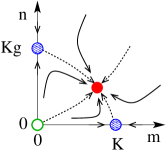
Figure 1: Schematic flow diagram in asymmetric two-species competition for weak competition in the mean field. The unstable node, the saddles, and the stable node are shown as open, hatched, and solid, respectively.

Extinction: The mean-field picture is incomplete because fluctuations of the population sizes about their fixed-point values are ignored. For large populations (corresponding to carrying capacity $K\gg 1$), these fluctuations are typically small. Thus the populations achieve a quasi-stationary state where the two species coexist. This state is stable in the mean-field description (heavy dot in Fig. 1). However, an unlikely sequence of deleterious events eventually occurs that ultimately leads one population, and then the other, to extinction. After the first extinction, the remaining population settles into another quasi-stationary state around one of the single-species fixed points $(m^{*},n^{*})=(K,0)$ or $(0,Kg)$. Eventually a large fluctuation drives the remaining species to extinction. This second extinction time is typically much longer [by a factor that scales as $\exp(\text{const.}\times K$)] than the first time, because the remaining species does not suffer interspecies competition. Once a species is extinct, there is no possibility of recovery since there is no replenishment mechanism.

The question that we address is: which species typically goes extinct first? The answer is encoded in the dynamics of the two-species probability $P_{m,n}(t)$. During the initial relaxation stage, a quasi-stationary probability distribution is quickly reached (Fig. 2). The probability distribution is sharply peaked at the stable fixed point of the mean-field theory. This probability slowly “leaks” into localized regions near each of the single-species fixed points $(m^{*},n^{*})=(K,0)$ and $(0,Kg)$. Thus two sharply-peaked single-species distributions start to form. If the $(K,0)$ peak grows faster then the B species is more likely to go extinct first. Similarly, a faster growing $(0,Kg)$ peak means A extinction is more likely. Eventually, the probability distribution that is localized at one of the two single-species fixed points slowly leaks toward the fixed point $(0,0)$ that corresponds to complete extinction movie .

To determine extinction rates, it is helpful to define $\mathcal{P}_{A}$, $\mathcal{P}_{B}$, and $\mathcal{P}_{\phi}$ as the respective probabilities that species A is extinct, species B is extinct, or neither is extinct at time $t$ GM12 . (Being interested in times much shorter than the expected extinction time of both species, we can neglect the probability of the latter process.) By definition, these extinction probabilities are

$$\mathcal{P}_{A}\!=\!\sum_{n>0}\!P_{0,n},\quad\mathcal{P}_{B}\!=\!\sum_{m>0}\!\!P_{m,0},\quad\mathcal{P}_{\phi}\!=\!\!\!\sum_{m,n>0}\!\!\!P_{m,n};$$ (6)

these satisfy $\mathcal{P}_{A}+\mathcal{P}_{B}+\mathcal{P}_{\phi}=1$, up to an exponentially small correction that stems from the process where both species become extinct simultaneously. In the limit $K\gg 1$ and for times much greater than the relaxation time scale $\tau_{r}$, the sums in Eqs. (6) are dominated by contributions from values of $m$ and $n$ that are close to the single-species and coexistence fixed points. Moreover, these extinction probabilities evolve according to a set of effective coupled equations

$$\begin{split}\dot{\mathcal{P}}_{A}&=R_{A}\mathcal{P}_{\phi}\,,\\ \dot{\mathcal{P}}_{B}&=R_{B}\mathcal{P}_{\phi}\,,\\ \dot{\mathcal{P}}_{\phi}&=-(R_{A}+R_{B})\mathcal{P}_{\phi}\,,\end{split}$$ (7)

that define $R_{A}$ and $R_{B}$ as the respective extinction rates for species A and species B. Solving these equations yields the time dependence of the extinction probabilities

$$\mathcal{P}_{A}(t)=\frac{R_{A}}{\mathcal{R}}\big{(}1\!-\!e^{-\mathcal{R}t}\big{)}\,,\quad\mathcal{P}_{B}(t)=\frac{R_{B}}{\mathcal{R}}\big{(}1\!-\!e^{-\mathcal{R}t}\big{)}\,,$$ (8)

with $\mathcal{R}=R_{A}+R_{B}$. To determine $R_{A}$ and $R_{B}$, we follow the evolution of the eigenstate of the master equation (Survival of the Scarcer) that determines the leakage of probability from the vicinity of the coexistence point:

$$P_{m,n}(t)=\Pi_{m,n}\,e^{-\mathcal{R}t},\qquad m,n>0,$$ (9)

where

$$\hat{H}\,\Pi_{m,n}=-\mathcal{R}\,\Pi_{m,n},\qquad m,n>0,$$ (10)

and $\mathcal{R}$ is the third-lowest positive non-trivial eigenvalue of the operator $\hat{H}$. The two still-smaller positive non-trivial eigenvalues correspond to the much slower decay of quasi-stationary single-species states and play no role in the dynamics of the first extinction event. There is also a trivial eigenvalue that corresponds to the final state of complete extinction.

Combining Eq. (Survival of the Scarcer) with (6)–(9), we obtain the following expression for the extinction rate of the A species:

$$R_{A}=\frac{1}{K}\sum_{n>0}\big{(}\epsilon\,n\,\Pi_{1,n}+\Pi_{2,n}\big{)}\,.$$ (11a)

As expected, the extinction rate for As involves two processes: (i) elimination of the last remaining A via competition with Bs and (ii) annihilation of the last remaining pair of As. Similarly,

$$R_{B}=\frac{1}{K}\sum_{m>0}\big{(}\alpha\epsilon\,m\,\Pi_{m,1}+\Pi_{m,2}\big{)}\,.$$ (11b)

To calculate $R_{A}$ and $R_{B}$, we therefore need to evaluate the small-population-size tails of $\Pi_{m,n}$. This task can be achieved by applying a variant of Wentzel-Kramers-Brillouin (WKB) approximation, that was pioneered in Refs. Kubo ; Hu ; Peters ; DykmanPRE100 , and was applied more recently to population extinction, in particular, for stochastic two-population systems DykmanPRL101 ; MeersonPRE77 ; MS09 ; KhasinPRL103 ; MeersonPRE81 ; LM2011 ; BM11 ; GM12 ; KMKS . The WKB ansatz for $\Pi_{m,n}$ has the form

$$\Pi_{m,n}=e^{-KS(x,y)},$$ (12)

where $x=m/K$ and $y=n/K$ are treated as continuous variables. Substituting Eq. (12) into (11a) and assuming $K\gg 1$, gives, to lowest order in $1/K$

$$R_{A}\sim e^{-KS_{A}}\,,\qquad\qquad R_{B}\sim e^{-KS_{B}}\,,$$ (13)

where $S_{A}=S(0,g)$ and $S_{B}=S(1,0)$, (see Refs. DykmanPRL101 ; MeersonPRE77 ; MS09 ; GM12 ). Thus as $K\gg 1$, the eventual extinction probabilities in (8) simply become (up to pre-exponential factors that depend on $K$), as

$$\mathcal{P}_{A}(t\!=\!\infty)=1\!-\!\mathcal{P}_{B}(t\!=\!\infty)\simeq\frac{e^{-KS_{A}}}{e^{-KS_{A}}\!+\!e^{-KS_{B}}}~{}.$$ (14)

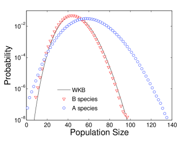
Figure 2: Quasi-stationary probability distributions for species A, $P_{m}=\sum_{n}P_{m,n}$, and species B, $P_{n}=\sum_{m}P_{m,n}$. Parameters are $K=100$, $\epsilon=0.9$, $g=0.45$, and $\alpha=0$. Symbols are simulation results, while the solid curve is WKB approximation for the B species distribution.

To determine the extinction probabilities explicitly, we therefore need $S_{A}$ and $S_{B}$. To this end, we substitute the WKB ansatz (12) in Eq. (10) and Taylor expand $S(x,y)$ to lowest order in $1/K$. After some algebra, we obtain an effective Hamilton-Jacobi equation $H(x,y,\partial_{x}S,\partial_{y}S)=-\mathcal{R}$, with the Hamiltonian

$$\begin{split}H(x,y,p_{x},p_{y})&=x(e^{p_{x}}\!-\!1)+gy(e^{p_{y}}\!-\!1)\\ &+\!\frac{x^{2}}{2}(e^{-2p_{x}}\!-\!1)\!+\!\frac{y^{2}}{2}(e^{-2p_{y}}\!-\!1)\\ &+\epsilon xy(e^{-p_{x}}\!-\!1)\!+\!\alpha\epsilon xy(e^{-p_{y}}\!-\!1)\,.\end{split}$$ (15)

Here $p_{x}=\partial_{x}S$ and $p_{y}=\partial_{y}S$ are the canonical momenta that are conjugate to the “coordinates” $x$ and $y$. Correspondingly, $S(x,y)$ is the classical action of the system.

Since we expect that $-\mathcal{R}$ (which now has the meaning of energy in this Hamiltonian system) is expected to be exponentially small, we set it to zero. The Hamiltonian equations of motion $\dot{x}=\partial H/\partial p_{x}$, $\dot{p}_{x}=-\partial H/\partial x$, etc., have six finite zero-energy fixed points, and three more fixed points where one or both momenta are at minus infinity. Only three of the fixed points, however, turn out to be relevant for answering our question about which species typically goes extinct first. These are:

$$\begin{split}F_{\phi}&=\left(\frac{1-g\epsilon}{1-\alpha\epsilon^{2}},\frac{g-\alpha\epsilon}{1-\alpha\epsilon^{2}},0,0\right)\,,\\ F_{A}&=\left(0,g,\ln(g\epsilon),0\right)\,,\\ F_{B}&=\left(1,0,0,\ln(\alpha\epsilon/g)\right)\,.\end{split}$$ (16)

A straightforward way to determine $S_{A}$ and $S_{B}$ is by calculating the action along the activation trajectories. These are zero-energy, but non-zero-momentum trajectories of the Hamiltonian system (15) that go from $F_{\phi}$ to $F_{A}$, and from $F_{\phi}$ to $F_{B}$, respectively. These actions are

$$S_{A}=\int_{F_{\phi}}^{F_{A}}(p_{x}dx+p_{y}dy)\,,$$ (17)

and similarly for $S_{B}$. In general, these activation trajectories—separatrices, or instantons—cannot be calculated analytically because of the lack of an integral of motion that is independent of the energy. However, for $\epsilon\ll 1$ a perturbative solution for these trajectories is possible.

As a preliminary, we outline how to calculate the action for the special case $\epsilon=0$, which corresponds to two uncoupled species. Here the zero-energy activation trajectories can be easily found. For the $F_{\phi}\rightarrow F_{A}$ separatrix, the B species is unaffected by A extinction so $(y,p_{y})$, which correspond to the coordinates of the Bs, remains constant throughout the evolution. As a result, a parametric form of the $F_{\phi}\rightarrow F_{A}$ separatrix is

$$x=\frac{2e^{2p_{x}}}{e^{p_{x}}\!+\!1},$$ (18a)

with $$y=g p_{y}=0 F_{\phi}\rightarrow F_{B}$$ and throughout. Similarly, for the separatrix one obtains

$$y=\frac{2ge^{2p_{y}}}{e^{p_{y}}\!+\!1},$$ (18b)

with $x=1$ and $p_{x}=0$ throughout. Substituting the trajectories given in (18) into (17) and performing the integration by parts gives $S_{A}=2(1-\ln 2)$ and $S_{B}=2g(1-\ln 2)$ EK ; KS07 .

For weak interspecies competition ($\epsilon\ll 1$), we can calculate the corrections to the actions to first order in $\epsilon$. For this purpose, we split the Hamiltonian (15) into unperturbed and perturbed parts, $H=H_{0}+\epsilon H_{1}$, and similarly expand the action as $S=S_{0}+\epsilon S_{1}+\dots$. Following DykmanPRL101 ; AKM08 ; KhasinPRL103 , the correction to the action is $S_{1}=\int_{-\infty}^{\infty}H_{1}[x(t),y(t),p_{x}(t),p_{y}(t)]dt$, where the integral is evaluated along the unperturbed trajectories given by Eqs. (18). Performing this integral for $S_{1}$ yields the corrected actions

$$\begin{split}S_{A}&=2(1-\ln 2)-\epsilon(2g\ln 2)\,,\\ S_{B}&=2g(1-\ln 2)-\epsilon(2\alpha\ln 2)\,.\end{split}$$ (19)

Equations (13) and (19) give the analytic expression for the extinction probabilities of each species for weak interspecies competition. Using Eq. (19) and imposing the condition $S_{A}=S_{B}$ from Eq. (14), we obtain the following condition for equal extinction probability for both species:

$$g=\frac{1+\alpha\,c\,\epsilon}{1+c\,\epsilon}~{},$$ (20)

where $c=\big{[}(\ln 2)^{-1}\!-\!1\big{]}^{-1}$. The predictions of Eqs. (14) and (19) are in good agreement with our simulation results (Fig. 3).

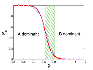
Figure 3: Probability that species B first becomes extinct as a function of growth rate asymmetry $g$ for $\alpha=0$, $\epsilon=0.1$, $K=40$. The curve is the prediction of Eq. (14), with actions given by (19), while circles are simulation results. In the hatched region, the quasi-stationary population of B is less than that of A, but Bs are less likely to become extinct first.

Phase Diagram: Comparing Eqs. (5) and (20), one sees that there is a sizable region in the $\alpha$-$g$ parameter space where one species has a smaller quasi-stationary population and yet an (exponentially) smaller probability to first become extinct. As an illustration, Fig. 3 shows the probability for B to become extinct first for fixed $\alpha$ and $\epsilon$. We also produced analogous curves as Fig. 3 at many values of $\alpha$. From the value of $g$ at which the extinction probabilities are equal, we infer the phase diagram shown in Fig. 4. Simulations at larger values of $\epsilon$ yield the same qualitative phase diagram.

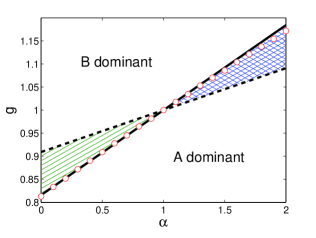
Figure 4: Phase diagram for $\epsilon=0.1$ showing loci of equal quasi-stationary population sizes (dashed) and equal extinction probabilities from Eq. (20) (solid). Circles indicate simulation results. In the hatched region, As are more numerous in the quasi-stationary state but are more likely to become extinct first. In the cross-hatched region Bs are more numerous but are more likely to become extinct first.

Conclusion: In two-species competition, interspecies competitive asymmetry leads to the unexpected phenomenon of “survival of the scarcer”. The very same elemental reactions that lead to a disadvantage in the quasi-stationary population size of one species within a deterministic mean-field theory, may also give this species a great advantage in its long-term survival when fluctuation effects are properly accounted for.

AG and SR gratefully acknowledge NSF grant DMR-0906504 and DMR-1205797 for partial financial support. BM was partially supported by the Israel Science Foundation (Grant No. 408/08), by the US-Israel Binational Science Foundation (Grant No. 2008075), and by the Condensed Matter Theory Visitors Program in the Boston University Physics Department.

References

- (1) J. D. Murray, Mathematical Biology I: An Introduction, 3rd ed. (Springer, New York, 2001).
- (2) G. Hardin, Science, 131, 1292 (1960).
- (3) J. C. Flores, J. Theor. Biol. 191, 295 (1988).
- (4) J. Bengtsson, Nature 340, 713 (1989).
- (5) A. E. Noble and W. F. Fagan, arXiv:1102.0052v1.
- (6) D. Gravel, F. Guichard, and M. E. Hochberg, Ecol. Lett. 14, 828 (2011).
- (7) T. L. Parsons and C. Quince, Theor. Popul. Biol. 72, 121 (2007).
- (8) N. G. Van Kampen, Stochastic Processes in Physics and Chemistry, ed. (North-Holland, Amsterdam, 2001).
- (9) See Supplemental Material at http://physics.bu.edu/~redner/pubs/pdf/weaker-sm.pdf, which contains a movie that shows the time evolution of .
- (10) O. Gottesman and B. Meerson, Phys. Rev. E, 85, 021140 (2012).
- (11) R. Kubo, K. Matsuo, and K. Kitahara, J. Stat. Phys. 9, 51 (1973).
- (12) G. Hu, Phys. Rev. A 36, 5782 (1987).
- (13) C. S. Peters, M. Mangel, and R. F. Costantino, Bull. Math. Biol. 51, 625 (1989).
- (14) M. I. Dykman, E. Mori, J. Ross, and P. M. Hunt, J. Chem. Phys. 100, 5735 (1994).
- (15) M. I. Dykman, I. B. Schwartz, and A. S. Landsman, Phys. Rev. Lett. 101, 078101 (2008).
- (16) A. Kamenev and B. Meerson, Phys. Rev. E 77, 061107 (2008).
- (17) B. Meerson and P. V. Sasorov, Phys. Rev. E 80, 041130 (2009).
- (18) M. Khasin and M. I. Dykman, Phys. Rev. Lett. 103, 068101 (2009).
- (19) M. Khasin, M. I. Dykman, and B. Meerson, Phys. Rev. E 81, 051925 (2010).
- (20) I. Lohmar and B. Meerson, Phys. Rev. E 84, 051901 (2011).
- (21) A. J. Black and A. J. McKane, J. Stat. Phys. P12006 (2011).
- (22) M. Khasin, B. Meerson, E. Khain, and L. M. Sander, Phys. Rev. Lett. 109, 138104 (2012).
- (23) V. Elgart and A. Kamenev, Phys. Rev. E 70, 041106 (2004).
- (24) D. A. Kessler and N. M. Shnerb, J. Stat. Phys. 127, 5 (2007).
- (25) M. Assaf, A. Kamenev, and B. Meerson, Phys. Rev. E, 78, 041123 (2008).