Spin modulation instabilities and phase separation dynamics in trapped two-component Bose condensates

Abstract

In the study of trapped two-component Bose gases, a widely used dynamical protocol is to start from the ground state of a one-component condensate and then switch half the atoms into another hyperfine state. The slightly different intra-component and inter-component interactions can then lead to highly nontrivial dynamics. We study and classify the possible subsequent dynamics, over a wide variety of parameters spanned by the trap strength and by the inter- to intra-component interaction ratio. A stability analysis suited to the trapped situation provides us with a framework to explain the various types of dynamics in different regimes.

I Introduction

Two-component Bose-Einstein condensates (BECs) are increasingly appreciated as a rich and versatile source of intricate non-equilibrium pattern dynamics phenomena. In addition to experimental observations MatthewsWiemanCornell_PRL98 ; HallWiemanCornell_PRL98 ; MiesnerStamper-KurnStenger_PRL99 ; ModugnoRiboliRoatiInguscio_PRL02 ; LewadowskiCornell_PRL02 ; MertesKevrekidisHall_PRL07 ; PappWieman_PRL08 ; vanDruten_expt ; HamnerEngelsHoefer_PRL11 ; Treutlein_NatPhys09 ; AndersonTicknorSidorovHall_PRA09 ; EgorovDrummondSidorov_PRA11 ; MyattCornellWieman_PRL97 , pattern dynamics in two-component BECs has attracted significant theoretical interest (see, e.g., HoShenoy_PRL96 ; LawPuBigelowEberly_PRL97 ; BuschCiracGarciaZoller_PRA97 ; PuBigelow_PRL98 ; Timmermans_PRL98 ; GrahamWalls_PRA98 ; SinatraFedichevCastinDalibardShlyapnikov_PRL99 ; KasamatsuTsubota_PRL04 ; KasamatsuTsubota_PRA06 ; Ronen_PRA08 ; NavarroKevrekidis_PRA09 ; WenLiuCaiZhangHu_PRA12 ; ZurekDavis_PRL11 ; LiTreutleinSinatra_EPJB09 ; BalazNicolin_PRA12 and citations in NavarroKevrekidis_PRA09 ).

In a number of two-component BEC experiments reported over more than a decade, a standard technique has been to start from the equilibrium state of a single-component BEC, e.g., populating a single hyperfine state of ⁸⁷Rb, and then using a $\pi/2$ pulse to switch half the atoms to a different hyperfine state HallWiemanCornell_PRL98 ; MatthewsWiemanCornell_PRL98 ; MiesnerStamper-KurnStenger_PRL99 ; LewadowskiCornell_PRL02 ; MertesKevrekidisHall_PRL07 ; vanDruten_expt ; EgorovDrummondSidorov_PRA11 ; AndersonTicknorSidorovHall_PRA09 ; Treutlein_NatPhys09 . This results in a binary condensate where the two intra-species interactions ($g_{11}$ and $g_{22}$) and one inter-species interaction ($g_{12}$) are all slightly different from each other, but the starting state is the ground state determined by $g_{11}$ alone. Since it has been realized several times in several different laboratory setups, this is a paradigm non-equilibrium initial state for binary condensate dynamics. A thorough and general analysis of the dynamics subsequent to such a $\pi/2$ pulse is thus clearly important. In this article we present such an analysis, clarifying the combined role of the inter-species interaction ($g_{12}$) and the strength $\lambda$ of the trapping potential. We provide a stability analysis mapping out regions of the $\lambda$–$g_{12}$ parameter space hosting different types of dynamics. Since it is now routine to monitor real-time dynamics in such experiments (e.g. vanDruten_expt ), we also directly analyze the real-time evolution after a $\pi/2$ pulse.

It is widely known that the ground state of a uniform two-species BEC is phase separated or miscible depending on whether or not the inter-species repulsion dominates over the self-repulsions of the two species, i.e., if

$$g_{11}g_{22}~{}<~{}\left(g_{12}\right)^{2}$$ (1)

then the ground state is phase separated HoShenoy_PRL96 . This criterion is also a key ingredient in understanding dynamical features such as pattern dynamics in the density difference between the two species — such “spin patterns” emerge when the phase separation condition is satisfied. This can be understood as the onset of a modulation instability Timmermans_PRL98 ; KasamatsuTsubota_PRL04 ; KasamatsuTsubota_PRA06 , identified by the appearance of an unstable mode in the excitation spectrum around a reference stationary state. For a homogeneous situation, linear stability analysis shows that modulation instability sets in when the condition of Eq. (1) is satisfied Timmermans_PRL98 ; KasamatsuTsubota_PRL04 ; KasamatsuTsubota_PRA06 .

The situation is different in the presence of a trapping potential. Phase separation in the ground state, as well as the appearance of modulation instability when starting from a mixed state, now requires larger inter-species repulsion NavarroKevrekidis_PRA09 ; WenLiuCaiZhangHu_PRA12 . This suggests that the region of parameter space where pattern dynamics occurs also depends on the trap. A trap is almost always present in cold-atom experiments, and it is easy to imagine experiments where the trapping potential is not extremely shallow but varies between tight and shallow limits. It is thus necessary to examine the relevance of Eq. (1) for trapped binary BECs. To this end, we explore different trap strengths spanning several orders of magnitude, and identify the appropriate extensions of Eq. (1) for the type of spin dynamics resulting from the $\pi/2$ protocol described above.

We focus on the effects of two parameters. First, we study effects of changing cross-species interaction $g_{12}$, thus generalizing Eq. (1) for trapped situations. Second, we explore the role of the relative strength of the trap with respect to the interactions. Our analysis, performed for a one-dimensional (1D) geometry, sheds light on the situation where $g_{11}$ and $g_{22}$ are close but unequal: (a) the stability analysis is performed for $g_{11}=g_{22}$ and their difference serves only to select appropriate instability modes; (b) the simulations are performed with $g_{22}/g_{11}=1.01$.

In Section II, we introduce the formalism and geometry. In Section III, we show results from a linear stability analysis for a sequence of trap strengths, and identify and analyze relevant modulation instabilities. Through an analysis of unstable modes, we present a classification of the parameter space into dynamically distinct regions, in relation to the prototypical initial state explained above. This may be regarded as a dynamical “phase diagram”. A remarkable aspect is that the “phase transition” line most relevant to spin pattern dynamics does not arise from the first modulation instability (studied in Ref. NavarroKevrekidis_PRA09 ). This first instability mode is antisymmetric in space, and as a result is not naturally excited in a symmetric trap with symmetric initial conditions. Complex dynamics (not due to collective modes but rather due to modulation instability) is generated only when the first spatially symmetric mode becomes unstable, which occurs at a higher value of $g_{12}$.

In Section IV we provide a relatively detailed account of the time evolution. For each trap strength $\lambda$, for values of $g_{12}$ not much larger than $g_{11}$, we observe simple collective modes. Above a threshold value of $g_{12}$, the oscillation amplitude becomes sharply stronger, and at the same time the motion becomes notably aperiodic, signaling that the dynamics is more complex than a combination of a few modes. Dynamical spin patterns start appearing at this stage and become more pronounced as $g_{12}$ is increased further. The threshold value at which the dynamics changes sharply corresponds to the second modulation instability line rather than the first, as we demonstrate through careful choice of parameters in each region of the phase diagram derived from stability analysis.

Some further connections between the stability analysis and dynamical features, relating to the length scale of generated patterns, appear in Section V. In the concluding Section VI we place our results in context and point out open questions.

II Geometry and formalism

The relevant time-resolved experiments have been performed in both quasi-1D geometries (highly elongated traps with strong radial trapping) vanDruten_expt and in a 3D BEC of cylindrical symmetry with the radial variable playing analogous role as the 1D coordinate HallWiemanCornell_PRL98 ; MertesKevrekidisHall_PRL07 . Since the basic phenomena are very similar, we expect the same theoretical framework to describe the essential features of each case. For definiteness, in this work we show results for 1D geometry. We expect the general picture emerging from this work to be qualitatively true also for other geometries exhibiting the same type of spin dynamics.

We describe the dynamics in the mean field framework at zero temperature, i.e., by two coupled Gross-Pitaevskii equations pitaevskii-jetp13 ; gross-nc20 ; SalasnichParolaReatto_PRA02 :

$$i\partial_{t}\psi_{1} = \bigg{(}-\tfrac{1}{2}\partial^{2}_{x}+\tfrac{1}{2}\lambda^{2}x^{2}+g_{11}|\psi_{1}|^{2}+g_{12}|\psi_{2}|^{2}\bigg{)}\psi_{1}\,,$$ (2)

$$i\partial_{t}\psi_{2} = \bigg{(}-\tfrac{1}{2}\partial^{2}_{x}+\tfrac{1}{2}\lambda^{2}x^{2}+g_{12}|\psi_{1}|^{2}+g_{22}|\psi_{2}|^{2}\bigg{)}\psi_{2}\,.$$ (3)

Condensate wave functions $\psi_{1}(x,t)$ and $\psi_{2}(x,t)$ are normalized to unity, and $\lambda$ is the strength of the harmonic trap. Factors of particle number and radial trapping frequency are absorbed as appropriate into the effective 1D interaction parameters $g_{ij}$ Olshanii_PRL98 ; SalasnichParolaReatto_PRA02 ; vanDruten_expt . We consider purely non-dissipative dynamics, i.e., we do not attempt to model experimental loss rates with a phenomenological dissipative term as done in, e.g., Refs. MertesKevrekidisHall_PRL07 ; vanDruten_expt ; AndersonTicknorSidorovHall_PRA09 .

The equations above are in dimensionless form because we measure lengths in units of trap oscillator length and time in units of inverse trapping frequency, for a hypothetical trap of unit strength ($\lambda=1$). The scale for trap strengths is itself fixed by imposing $g_{11}=1$. With this convention, small values of $\lambda$ correspond to a BEC in the Thomas-Fermi limit. For comparison, we note that the parameters of the experiment of Ref. vanDruten_expt corresponds to $\lambda$ of order $10^{-5}$ in these units. Of course one can switch between different units via the transformation: $x\rightarrow x/l$, $t\rightarrow t/l^{2}$, $\lambda\rightarrow\lambda l^{2}$, $g\rightarrow gl$, and $\psi\rightarrow\psi\sqrt{l}$, where $l$ is an appropriately chosen scale.

The initial state after a $\pi/2$ pulse involves both components occupying the ground state of a single-component system of interaction $2g_{11}$, because the atoms were all in the first hyperfine state before the pulse. We model this initial situation as a two-component BEC with $g_{11}=g_{22}=g_{12}$. The $\pi/2$ pulse may then be regarded as a sudden change (a quantum quench PolkovnikovSengupta_RMP11 ) of the interaction parameters $g_{22}$ and $g_{12}$.

We use $g_{11}=g_{22}$ for the stability analysis of Section III. For the explicit time evolution reported in Section IV, we use $g_{11}$ and $g_{22}$ values close but unequal: $g_{11}=1$, $g_{22}=1.01$. This choice of close values is convenient for illustrating the structure of the phase diagram, especially for shallow traps. In rubidium experiments the difference between $g_{11}$ and $g_{22}$ is somewhat larger (in the common case using ⁸⁷Rb hyperfine states $\left|{1}\right.\rangle=\left|{F=1,m_{F}=-1}\right.\rangle$ and $\left|{2}\right.\rangle=\left|{F=2,m_{F}=1}\right.\rangle$); however our insights should be relevant to a broad regime of possible experiments. A full exploration of the regime of arbitrary differences ($g_{11}-g_{22}$) remains an open task, beyond the scope of the present manuscript.

Numerical simulations presented in Section IV were performed using a semi-implicit Crank-Nicolson method sicn ; IvanaAntun_2012 .

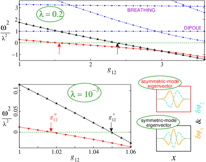
Figure 1: (Color online.) Results from stability analysis. Squared eigenvalues $\omega^{2}$ of the stability matrix $\mathcal{M}$ are plotted against $g_{12}$, for a tight trap (top) and for a shallow trap (bottom left). The arrows show the values of $g_{12}$ for onset of the two instabilities, namely $g_{12}^{a}$ (onset of spatially antisymmetric modulation instability) and $g_{12}^{s}$ (onset of spatially symmetric instability). Typical eigenvectors corresponding to these two modes are shown in the panels on lower right.

III Stability analysis and dynamical “phase diagram”

We provide in this section a stability analysis for $g_{11}=g_{22}$ that maps out the regions of $\lambda$-$g_{12}$ parameter space which support pattern formation instabilities.

Ideally, one might like to perform a stability analysis around the initial state. However, in contrast to the homogeneous case Timmermans_PRL98 , we are faced with the situation that the initial state is not a stationary state of the final Hamiltonian. The choice of reference state is therefore a somewhat subtle aspect of the present analysis.

We use as reference state $\psi_{0}(x)$ the lowest-energy spatially symmetric stationary state of the case $g_{11}=g_{22}$, with parameter $g_{12}$ set to its final value. (For large $g_{12}$, this is not the ground state for these parameters, which is phase-separated.) This reference state has the advantage of looking relatively similar to our actual initial state (two components totally overlapping in space), and of being a stationary state of the Hamiltonian for which we analyze linear stability. Our reference state can be regarded as placing both components in the single-component ground state for interaction $g_{11}+g_{12}$. We are not aware of a suitable stationary state even more similar to the actual initial state. We will see that our stability analysis around this reference state will predict remarkably well the main observed time-evolution features described in Section IV.

Note that it is not natural to use $g_{11}\neq g_{22}$, because stationary states for such a case typically do not overlap completely in space. Instead, in our approach the difference between $g_{11}$ and $g_{22}$ will play the important role of selecting certain instability modes over others. For this reason, inferences from the present analysis apply only to small relative differences between $g_{11}$ and $g_{22}$.

We linearize Eqs. (2) and (3) around the reference stationary state $\psi_{0}(x)$:

$$\psi_{1}(x,t)=\left[\psi_{0}(x)+\delta\psi_{1}(x,t)\right]\exp(-i\mu t),$$

$$\psi_{2}(x,t)=\left[\psi_{0}(x)+\delta\psi_{2}(x,t)\right]\exp(-i\mu t),$$ (4)

where $\mu$ is the chemical potential corresponding to the reference state. By keeping only terms of the first order in $\delta\psi_{1}(x,t)$ and $\delta\psi_{2}(x,t)$, we obtain a system of linear equations which can be cast in the form:

$$\partial_{t}^{2}\begin{pmatrix}\delta\psi_{1}+\delta\psi_{1}^{*}\\ \delta\psi_{2}+\delta\psi_{2}^{*}\end{pmatrix}+\mathcal{M}\begin{pmatrix}\delta\psi_{1}+\delta\psi_{1}^{*}\\ \delta\psi_{2}+\delta\psi_{2}^{*}\end{pmatrix}~{}=~{}0.$$ (5)

Here $\mathcal{M}$ is a matrix differential operator which, upon discretization or upon expansion in a set of orthogonal functions, becomes the so-called stability matrix (e.g., PuBigelow_PRL98 ; LawPuBigelowEberly_PRL97 ). We analyze below the eigenmodes of the stability matrix, which we have obtained by numerically calculating the reference stationary state $\psi_{0}(x)$ and expanding in the basis of harmonic trap (non-interacting) eigenstates.

Since we use $g_{11}=g_{22}$ for the stability analysis, eigenmodes will have well-defined “species parity”, i.e. will all be either even [$\delta\psi_{1}(x,t)=\delta\psi_{2}(x,t)$] or odd [$\delta\psi_{1}(x,t)=-\delta\psi_{2}(x,t)$] with respect to the interchange of species. Even modes describe in-phase motion of the two components and simply correspond to the excitation spectrum of a single-component BEC with interaction constant $g_{11}+g_{12}$. Odd modes are more interesting — they describe out-of-phase motion of two components and are therefore reflected in the spin dynamics. Additionally, due to the spatial inversion symmetry $x\rightarrow-x$, the solutions will also have well-defined spatial parity, and we can distinguish spatially symmetric and antisymmetric modes.

Typical eigenspectra are presented in Fig. 1. In the case of a tight trap $\lambda=0.2$, we notice two modes whose frequencies are nearly constant. These are even modes encoding single-component or in-phase physics. The lower one is the dipole (Kohn) mode with frequency equal to the trap frequency $\lambda$. The second nearly-constant mode is the breathing mode, which for elongated traps takes value close to $\omega^{2}=3\lambda^{2}$. The breathing mode (oscillations of cloud size) is visible in the plots of Fig. 3 (Section IV) as a fast oscillation of the total condensate widths.

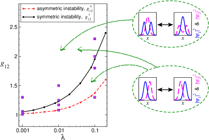
Figure 2: (Color online.) The dynamical “phase diagram” showing the critical values of $g_{12}$ for the onset of the two types of modulation instability versus the trap strength $\lambda$. The instability lines are shown as straight lines joining numerically determined values. The oscillation schematics on the right (and corresponding arrows) indicate that left-right-left oscillation modes are persistent everywhere above the $g_{12}^{a}$ line, while in-out-in modes are persistent only above the higher $g_{12}^{s}$ line. The spatially symmetric instability ($g_{12}^{s}$ line) is the one relevant for experimental situations with symmetric traps. Squares mark values used in the dynamical simulations of Figs. 3 and 4 (Table 1).

The two lowest-lying eigenmodes are odd modes encoding out-of-phase physics. For $g_{12}\gtrsim 1$, their frequencies are significantly below the breathing mode, and therefore lead to relatively slow oscillations in the spin density. This will also be visible in the real-time dynamics presented in Section IV (first two columns of Figs. 3 and 4). The forms of the corresponding eigenvectors are shown in the lower right of Fig. 1. The nature of the eigenvectors shows that the motion related to the lowest mode corresponds to the left-right oscillations of the two species, while the next odd mode corresponds to spatially symmetric spin motion. The frequencies of these two modes become imaginary at certain values of $g_{12}$, thus leading to the onset of modulation instabilities. The antisymmetric mode becomes unstable at smaller value of $g_{12}$ ($g_{12}^{a}\approx 1.6$ for $\lambda=0.2$) in comparison to the symmetric mode ($g_{12}^{s}\approx 2.4$ for $\lambda=0.2$). In a spatially symmetric trap, there is no natural mechanism for exciting the spatially antisymmetric mode. On the other hand, any difference between $g_{11}$ and $g_{22}$ naturally excites the second (spatially symmetric) mode. Thus, the second mode, occurring at larger $g_{12}$, is the relevant instability for understanding the dynamics observed in experiments and explored numerically in Section IV.

We find similar excitation spectra for trap strengths $\lambda$ spanning several orders of magnitude. The spatially antisymmetric mode becomes unstable before the spatially symmetric mode, and both instabilities get closer to 1 as the trap gets shallower. For example, for $\lambda=10^{-3}$ (also shown in Fig. 1) the lowest instability sets in for $g_{12}^{a}\approx 1.02$, while the next one appears at $g_{12}^{s}\approx 1.05$. The distinction between two instabilities becomes ever smaller as we go toward a uniform system $\lambda\rightarrow 0$, where the phase-separation condition Eq. (1) becomes exact. Nevertheless, even for shallow traps, the issue is not purely academic as the precision in experimental measurement and control of scattering lengths continues to improve vanDruten_expt ; EgorovOpanchuk12 .

In Fig. 2 (main panel), the results of the stability analyses are combined to present a dynamical “phase diagram”. The two lines show the two instabilities ($g_{12}^{a}$ and $g_{12}^{s}$) as a function of trap strength $\lambda$. For very shallow traps, the two transition lines merge as $g_{12}^{s}\approx g_{12}^{a}\approx 1$. The lower transition line ($g_{12}^{a}$) was previously introduced in Ref. NavarroKevrekidis_PRA09 . However, for a trap and initial state with left-right spatial symmetry, this is not the relevant dynamical transition line, because the first even mode only becomes unstable at some higher $g_{12}$ value, given by the $g_{12}^{s}$ line.

In the next Section, we will see that spin pattern dynamics is indeed only generated when the inter-component repulsion $g_{12}$ exceeds the second instability line ($g_{12}>g_{12}^{s}$), and that crossing the first instability ($g_{12}^{a}<g_{12}<g_{12}^{s}$) is not enough for pattern formation in a spatially symmetric trap.

IV Dynamical features across the parameter space

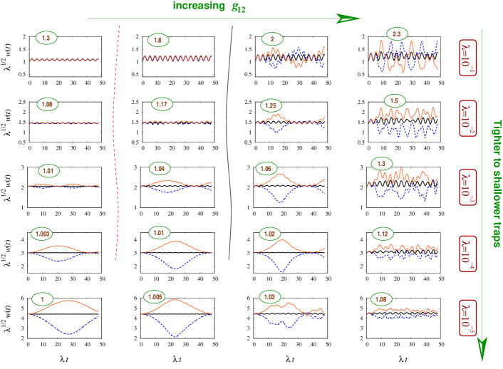
Figure 3: (Color online.) Time evolution of root-mean-square widths after $\pi/2$ pulse (interaction quench). First component width $w_{1}(t)$ is shown as blue dashed line, second component width $w_{2}(t)$ is shown as red solid line (gray solid without color), the total width $w(t)=\sqrt{(w_{1}^{2}(t)+w_{2}^{2}(t))/2}$ is the black solid line intermediate between the other two. From top to bottom: tight to shallow traps. For each trap strength, four values of $g_{12}$ (indicated near top of each panel) from Table 1 are used. The two lines separating first and second column (red dashed) and second and third column (black solid) indicate the ‘positions’ of instability lines, from Figure 2. While the first two columns look qualitatively the same and show regular oscillatory dynamics, in the third column we observe aperiodic motion of stronger amplitude that we relate to the onset of spin pattern dynamics. The spin dynamics is even more pronounced in the fourth column.

In this Section we present and analyze the dynamics obtained from direct numerical simulation of the Gross-Pitaevskii equations (2) and (3), after the system is initially prepared in the ground state of the situation $g_{11}=g_{22}=g_{12}=1$. The subsequent dynamics is performed with $g_{11}=1$, $g_{22}=1.01$, and several different values of $g_{12}$ for each trap strength $\lambda$.

$\lambda$	$\frac{g_{12}^{(1)}}{\sqrt{g_{11}g_{22}}}$	$\frac{g_{12}^{(2)}}{\sqrt{g_{11}g_{22}}}$	$\frac{g_{12}^{(3)}}{\sqrt{g_{11}g_{22}}}$	$\frac{g_{12}^{(4)}}{\sqrt{g_{11}g_{22}}}$	$g_{12}^{a}$	$g_{12}^{s}$
$10^{-1}$	1.3	1.8	2	2.3	1.37	1.92
$10^{-2}$	1.08	1.17	1.25	1.5	1.085	1.23
$10^{-3}$	1.01	1.04	1.06	1.3	1.018	1.050
$10^{-4}$	1.003	1.01	1.02	1.12	1.004	1.011
$10^{-5}$	1	1.005	1.03	1.08	$\approx$1	$\approx$1

Table 1: Parameters from the first five columns are used for the plots in Figs. 3 and Figs. 4. The instability values $g_{12}^{a}$ and $g_{12}^{s}$ (introduced in Figs. 1 and 2 and discussed in Section III) are also given for each trap strength.

It is difficult to show the full richness of pattern dynamics through plots of a few quantities. We choose to show the dynamics through two types of plots (Figs. 3 and 4). Fig. 3 shows the time dependence of the root mean square widths of the two components

$$w_{1,2}^{2}(t)=\int_{-\infty}^{\infty}x^{2}|\psi_{1,2}(x,t)|^{2}dx,$$ (6)

while Fig. 4 shows density plots of the density difference (spin density), $|\psi_{1}(x,t)|^{2}-|\psi_{2}(x,t)|^{2}$. In both figures, each row corresponds to a different trap strength ($\lambda$), and we approach the shallow trap (Thomas-Fermi) limit going from top to bottom.

For each $\lambda$ the four values of $g_{12}$ from Table 1 are used for Figs. 3 and 4. We have chosen $g_{12}$ values such that the first panel in each row is in the parameter region where there are no instabilities, the second one is in the region where the only instability is the antisymmetric one, and the third on each row is at $g_{12}$ values just above the second, relevant, instability. The fourth panel on each row is at higher $g_{12}$ values. The choice of $g_{12}$ values with respect to instability lines is clear in the tighter traps of the top three rows, as also shown by squares in Fig. 2. For shallow traps (lower rows), the instability lines are too close together and too close to $g_{12}=1$, so making such choices is not meaningful. In the following, as we compare features of the different columns, we implicitly exclude the lowest row (smallest $\lambda$). This is also indicated by the fact that the schematic instability lines in Figs. 3 and 4 are not extended to the lowest row.

Broadly speaking, we note that there is only regular (collective-mode) dynamics in the second-column figures ($g_{12}^{a}<g_{12}<g_{12}^{s}$) even though an instability is present. There is generally a sharp difference between the second and third figure in each row, indicating that the second instability ($g_{12}^{s}$) is the relevant one. The fourth panel on each row is at higher $g_{12}$ values, showing more rich dynamics.

In Fig. 3, we show time-dependence of the individual widths ($w_{1}$, $w_{2}$) and also of the total root mean square width, $w(t)=\sqrt{(w_{1}^{2}(t)+w_{2}^{2}(t))/2}$. Consistent with our observation that spatially symmetric modes (and not the antisymmetric ones) are naturally excited in the current setup, the dynamics shows signatures of the two most prominent spatially symmetric modes noted in Fig. 1. The breathing mode is the easiest to notice and most ubiquitous — it shows up in almost every parameter choice as oscillations in the total density (in-phase in the two components), with a typical period given by $2\pi/\sqrt{3}\lambda\approx 3.63/\lambda$. This follows from the frequency of this mode being almost constant near $\sqrt{3}\lambda$.

We also see out-of-phase motion of the two components, associated with the lower spatially-symmetric mode in Fig. 1, which has odd species parity. In the first two columns of Fig. 3, corresponding to smaller values of $g_{12}$ such that this mode has small real frequencies, this is excited as a regular ‘spin’ mode. For example, at $\lambda=10^{-3}$ and $g_{12}=1.04$, we observe an out-of-phase oscillation with the period of approximately $\approx 30$, much slower than the breathing mode. In addition, the oscillation period of the out-of-phase motion is slower in the second than in the first column of each row, corresponding to the decreasing frequency of the mode, as seen in stability analysis (Fig. 1). Once $g_{12}$ becomes large enough that the instability threshold for this mode is crossed, the oscillation amplitudes increase sharply and the width dynamics becomes strongly aperiodic and irregular (third column of Fig. 3). This signifies the onset of pattern dynamics, as opposed to the excitation of a regular collective mode around a stable state. Irregularity of the width dynamics at stronger $g_{12}$ is even more apparent in the fourth column of Fig. 3.

It is noteworthy that the spatially antisymmetric modes play no role and do not show up in these dynamical simulations. We see no signature of the Kohn mode. Nor do we see any sharp change associated with the instability of the antisymmetric mode, i.e., there is no sharp difference between the first two columns of Fig. 3.

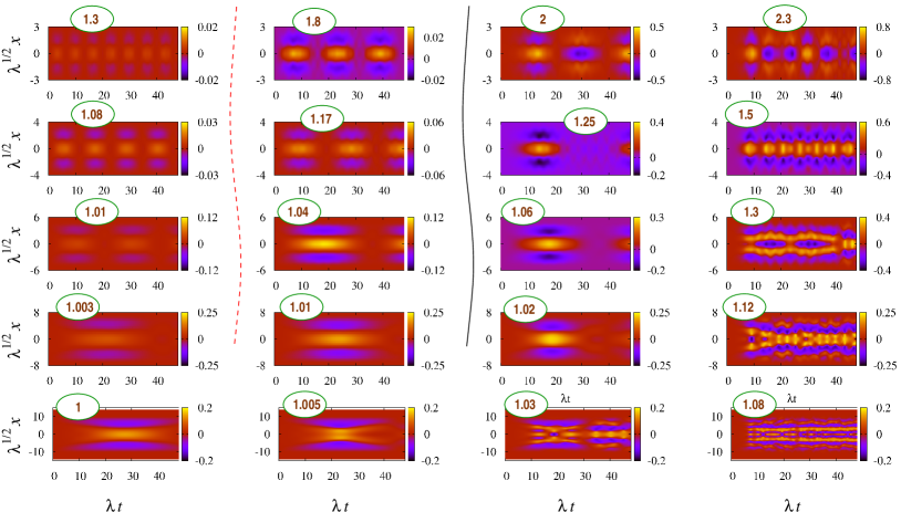
Figure 4: (Color online.) Spin dynamics subsequent to the $\pi/2$ protocol, shown via the density difference $\lambda^{-1/2}\left(|\psi_{1}(x,t)|^{2}-|\psi_{2}(x,t)|^{2}\right)$. Traps and $g_{12}$ values are the same as in Fig. 3 and Table 1: $\lambda$ decreases from $10^{-1}$ to $10^{-5}$ from top to bottom and $g_{12}$ values are indicated near top of each panel. As in Fig. 3, the black solid line and the red dashed line indicate the instability lines from the “phase diagram” of Fig. 2. Note the sharp change of color-scale ranges between second and third columns in the upper rows, indicating that the dynamics changes dramatically only across the second instability line.

In Fig. 4 we show the dynamics of the “spin density” $|\psi_{1}(x,t)|^{2}-|\psi_{2}(x,t)|^{2}$. The case of very shallow traps (last row), resembles the data in Refs. KasamatsuTsubota_PRL04 ; KasamatsuTsubota_PRA06 . As in Fig. 3, the first two columns show regular oscillations, corresponding to collective modes without instability. A sharp change occurs, not across the first instability line (between 1st and 2nd column), but instead across the second instability line (2nd and 3rd columns), especially for tighter traps (top three rows) where comparison with instability lines is meaningful. The sharp change can be noted through the color scales, which is dramatically different between second and third columns in the upper rows.

V Length Scales of patterns

In homogeneous stability analysis, the length scale of patterns is inferred from the wavevector (momentum) at which an instability first occurs. Since we perform our stability analysis specifically for trapped systems, we do not have a momentum quantum number. Nevertheless, the eigenvectors of the unstable modes contain information about the form of patterns generated in the dynamics of the trapped system. This is illustrated in Fig. 5, where the eigenvectors of the lowest unstable even-parity modes are shown for several values of $g_{12}$, together with the spin patterns generated in the non-equilibrium dynamics. There is a close match between the distance between nodes of the eigenvectors (rough analog of ‘wavevector’) and the length scales involved in the patterns.

In Fig. 4 we see that the patterns contain more spatial structure in shallow traps. The top two rows (tight traps) only show in-out-in type of patterns. This can be understood from the idea that the interactions induce length scales (‘healing lengths’) in the problem, which are smaller for larger interactions, and which set the length scale of spatial structures. For tight traps, the healing length set by the interactions is large or comparable to the cloud size, so that only global dynamical patterns are generated. In such traps, generation of complex patterns with many spatial oscillations would require much higher values of $(g_{12}/g_{11}-1)$. For shallow traps, the healing length becomes much smaller than the cloud size; as a result one can have a multitude of dynamical spin structures in the system, of the type seen in experiments and prior simulations KasamatsuTsubota_PRA06 ; vanDruten_expt ; MertesKevrekidisHall_PRL07 . This heuristic explanation can be made quantitative by counting the number of nodes appearing in the eigenmodes (as in Fig. 5).

VI Conclusions and Open Problems

In this article we have analyzed a widely used dynamical protocol for two-component BECs, which involves starting from the ground state of one component and switching half the atoms to a different component through a $\pi/2$ pulse. We have presented a stability analysis suitable to the trapped situation, and also presented results from extensive dynamical simulations. Through an analysis of unstable modes, we have presented a classification of the parameter space into a number of dynamically distinct regions, in relation to the prototypical initial state. This may be regarded as a dynamical “phase diagram”.

In the ‘stable’ regime of parameter space (no modulation instabilities), our stability analysis explains the observed slow spin oscillations compared to the fast breathing mode oscillations of the total density. We demonstrate that the important “phase transition” line for spatially symmetric situations relevant to most experiments is not the first instability (studied in Ref. NavarroKevrekidis_PRA09 ), but a second transition line. The first instability is antisymmetric in space, and as a result is not naturally excited in a symmetric trap.

Our stability analysis is performed relative to a stationary state of the situation $g_{11}=g_{22}$. The $\pi/2$ pulse of the experiments (in the cases where $g_{11}{\neq}g_{22}$) can be considered as turning on a nonzero $(g_{11}-g_{22})$, i.e., turning on ‘buoyancy’ such that one component gains more energy by being in the interior of the trap compared to the other. This helps to select instability modes which are symmetric in space.

Since we have used a stability analysis with $g_{11}=g_{22}$ to analyze dynamics with $g_{11}{\neq}g_{22}$, an obvious question is how the ratio $g_{22}/g_{11}$ affects the regime of applicability of this scheme. We expect that features of this ($g_{11}=g_{22}$) stability analysis are useful for dynamical predictions as long as $g_{12}/g_{11}-1$ is roughly more than $g_{22}/g_{11}-1$. For example, for shallow traps (small $\lambda$), the instabilities occur at $g_{12}/g_{11}-1$ values comparable to 0.01, which is why the placement of parameters in the three dynamical regions of the ‘phase diagram’ (Fig. 2) is not meaningful for the smallest $\lambda$ values (lowest rows of Figs. 3 and 4).

For the stability analysis we used a reference stationary state which is of course not the initial state: the initial state is the ground state for $g_{11}=g_{22}=g_{12}$, while the reference state is the lowest-energy spatially symmetric stationary state corresponding to the final value of $g_{12}$. The instability lines found in this stability analysis would describe even better a situation where the dynamics is triggered by a small quench of $g_{12}$, as opposed to the changes of $g_{12}$ that we consider here, which can be relatively large. We have looked at some examples of this type of dynamics and indeed find instabilities matching the stability analysis extremely well. However, although the initial state in the $\pi/2$ dynamics is somewhat different from the reference state of our stability analysis, our results show that this stability analysis does provide an excellent overall picture of the dynamics generated by the $\pi/2$ protocol.

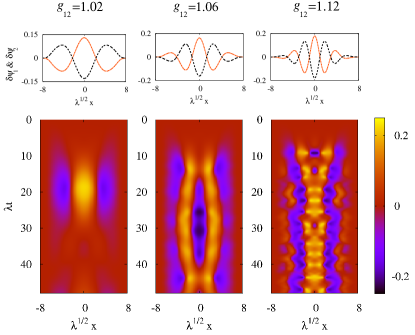
Figure 5: (Color online.) Top: Eigenvectors of the most unstable even eigenmodes, from the stability analysis of Section III, for $\lambda=10^{-4}$, and $g_{12}=1.02$, $1.06$, and $1.12$ from left to right. Below each eigenvector, the corresponding spin dynamics after the $\pi/2$ protocol (parameters of Section IV) is shown through the time evolution of $|\psi_{1}(x,t)|^{2}-|\psi_{2}(x,t)|^{2}$.

Our work opens up a number of questions deserving further study. First of all, we have thoroughly explored the $\lambda$–$g_{12}$ parameter space, while assuming that the intra-component interactions $g_{11}$ and $g_{22}$ are unequal but close in value. The regime of large difference ($g_{11}-g_{22}$) clearly might have other interesting dynamical features which are yet to be explored.

Second, in this work we have restricted ourselves to the mean field regime. While the mean field description captures well the richness of pattern formation phenomena (c.f. Refs. KasamatsuTsubota_PRL04 ; KasamatsuTsubota_PRA06 ; MertesKevrekidisHall_PRL07 ; Ronen_PRA08 ; NavarroKevrekidis_PRA09 in addition to present work), it may be worth asking whether quantum effects beyond mean field might have interesting consequences for the patter dynamics generated by a $\pi/2$ pulse. For bosons in elongated traps, regimes other than mean field (such as Lieb-Liniger or Tonks regimes) may occur naturally in experiments PetrovShlyapnikovWalraven_PRL00 ; FuchsGangardtShlyapnikov_PRL05 ; Weiss_tonksgas_Science04 ; NJvD_PRL08 ; Naegerl_excited_stronglycorrelated_Science09 . Dynamics subsequent to a $\pi/2$ pulse in strongly interacting 1D gases outside the mean field regime is an open area of investigation.

Third, we have assumed a spatially symmetric trap and an initial condition with spatial symmetry, and this plays a crucial role in the selection of instability channels. In a real-life experiment, the trap will have some left-right asymmetry. Also, thermal and quantum fluctuations can initiate spatially antisymmetric excitations. The extent to which a small spatial asymmetry affects spin dynamics remains unexplored; in such a case we would have some type of competition between two types of instabilities. Ref. NavarroKevrekidis_PRA09 has studied dynamical effects of fluctuations (noise), but the effects of thermal and quantum fluctuations is yet to be studied in the context of a $\pi/2$ protocol.

Finally, one could consider time evolution and spatiotemporal patterns generated by a $\pi/2$ pulse in the presence of an optical lattice, described by the dynamics of a two-component Bose-Hubbard model. This is a situation easy to imagine realizing experimentally. One could speculate complex interplay between spin dynamics and the spatial arrangement of Mott and superfluid regions.

- (1) M. R. Matthews, D. S. Hall, D. S. Jin, J. R. Ensher, C. E. Wieman, E. A. Cornell, F. Dalfovo, C. Minniti, and S. Stringari, Phys. Rev. Lett. 81, 243 (1998).
- (2) D. S. Hall, M. R. Matthews, J. R. Ensher, C. E. Wieman, and E. A. Cornell, Phys. Rev. Lett. 81, 1539 (1998).
- (3) H.-J. Miesner, D. M. Stamper-Kurn, J. Stenger, S. Inouye, A. P. Chikkatur, and W. Ketterle, Phys. Rev. Lett. 82, 2228 (1999).
- (4) H. J. Lewandowski, D. M. Harber, D. L. Whitaker, and E. A. Cornell, Phys. Rev. Lett. 88, 070403 (2002)
- (5) K. M. Mertes, J. W. Merrill, R. Carretero-González, D. J. Frantzeskakis, P. G. Kevrekidis, and D. S. Hall, Phys. Rev. Lett. 99, 190402 (2007).
- (6) P. Wicke, S. Whitlock, and N. J. van-Druten, arXiv:1010.4545.
- (7) R. P. Anderson, C. Ticknor, A. I. Sidorov, and B. V. Hall, Phys. Rev. A 80, 023603 (2009)
- (8) P. Boehi, M. F. Riedel, J. Hoffrogge, J. Reichel, T. W. Haensch, and P. Treutlein, Nat. Phys. 5, 592 (2009).
- (9) M. Egorov, R. P. Anderson, V. Ivannikov, B. Opanchuk, P. Drummond, B. V. Hall, and A. I. Sidorov, Phys. Rev. A 84, 021605 (2011).
- (10) S. B. Papp, J. M. Pino, and C. E. Wieman, Phys. Rev. Lett. 101, 040402 (2008).
- (11) C. J. Myatt, E. A. Burt, R. W. Ghrist, E. A. Cornell, and C. E. Wieman, Phys. Rev. Lett. 78, 586 (1997).
- (12) G. Modugno, M. Modugno, F. Riboli, G. Roati, and M. Inguscio, Phys. Rev. Lett. 89, 190404 (2002).
- (13) C. Hamner, J. J. Chang, P. Engels, and M. A. Hoefer, Phys. Rev. Lett. 106, 065302 (2011).
- (14) R. Navarro, R. Carretero-González, and P. G. Kevrekidis, Phys. Rev. A 80, 023613 (2009).
- (15) Tin-Lun Ho and V. B. Shenoy, Phys. Rev. Lett. 77, 3276 (1996).
- (16) E. Timmermans, Phys. Rev. Lett. 81, 5718 (1998).
- (17) K. Kasamatsu and M. Tsubota, Phys. Rev. Lett. 93, 100402 (2004)
- (18) K. Kasamatsu and M. Tsubota, Phys. Rev. A 74, 013617 (2006).
- (19) L. Wen, W. M. Liu, Y. Cai, J. M. Zhang, and J. Hu, Phys. Rev. A 85, 043602 (2012).
- (20) S. Ronen, J. L. Bohn, L. E. Halmo, and M. Edwards, Phys. Rev. A 78, 053613 (2008).
- (21) J. Sabbatini, W. H. Zurek, and M. J. Davis, Phys. Rev. Lett. 107, 230402 (2011).
- (22) C. K. Law, H. Pu, N. P. Bigelow, and J. H. Eberly, Phys. Rev. Lett. 79, 3105 (1997).
- (23) Th. Busch, J. I. Cirac, V. M. Perez-Garcia, and P. Zoller, Phys. Rev. A 56, 2978 (1997).
- (24) H. Pu and N. P. Bigelow, Phys. Rev. Lett. 80, 1134 (1998).
- (25) R. Graham and D. Walls, Phys. Rev. A 57, 484 (1998).
- (26) A. Sinatra, P. O. Fedichev, Y. Castin, J. Dalibard, and G. V. Shlyapnikov, Phys. Rev. Lett. 82, 251 (1999).
- (27) Y. Li, P. Treutlein, J. Reichel, and A. Sinatra, Eur. Phys. Journ. B 68, 365 (2009).
- (28) A. Balaž and A. Nicolin, Phys. Rev. A 85, 023613 (2012).
- (29) A. Polkovnikov, K. Sengupta, A. Silva, and M. Vengalattore, Rev. Mod. Phys. 83, 863 (2011).
- (30) L. P. Pitaevskii, Sov. Phys. JETP 13, 451 (1961).
- (31) E. P. Gross, Nuovo Cimento 20, 454 (1961).
- (32) L. Salasnich, A. Parola, and L. Reatto, Phys. Rev. A 65, 043614 (2002).
- (33) M. Olshanii, Phys. Rev. Lett. 81, 938 (1998).
- (34) P. Muruganandam and S. K. Adhikari, Comput. Phys. Commun. 180, 1888 (2010).
- (35) D. Vudragović, I. Vidanović, A. Balaž, P. Muruganandam, and S. K. Adhikari, Comput. Phys. Commun. 183, 2021 (2012).
- (36) M. Egorov, B. Opanchuk, P. Drummond, B. V. Hall, P. Hannaford, and A. I. Sidorov, arXiv:1204.1591.
- (37) D. S. Petrov, G. V. Shlyapnikov, and J. T. M. Walraven, Phys. Rev. Lett. 85, 3745 (2000).
- (38) J. N. Fuchs, D. M. Gangardt, T. Keilmann, and G. V. Shlyapnikov, Phys. Rev. Lett. 95, 150402 (2005).
- (39) A. H. van Amerongen, J. J. van Es, P. Wicke, K. V. Kheruntsyan, and N. J. van Druten, Phys. Rev. Lett. 100, 090402 (2008).
- (40) T. Kinoshita, T. Wenger, and D. S. Weiss, Science 305, 1125 (2004).
- (41) E. Haller M. Gustavsson, M. J.. Mark, J. G. Danzl, R. Hart, G. Pupillo, and H.-C. Nägerl, Science 325, 1224 (2009).