Short vs Long and Collapsars vs. non-Collapsar: a quantitative classification of GRBs.

Abstract

Gamma-Ray Bursts (GRBs) are traditionally divided to long and short according to their durations ($\lessgtr 2$ sec). It was generally believed that this reflects a different physical origin: Collapsars (long) and non-Collapsars (short). We have recently shown that the duration distribution of Collapsars is flat, namely independent of the duration, at short durations. Using this model for the distribution of Collapsars we determine the duration distribution of non-Collapsars and estimate the probability that a burst with a given duration (and hardness) is a Collapsar or not. We find that this probability depends strongly on the spectral window of the observing detector. While the commonly used limit of 2 sec is conservative and suitable for BATSE bursts, 40% of Swift ’s bursts shorter than 2 sec are Collapsars and division $\lessgtr 0.8$ sec is more suitable for Swift . We find that the duration overlap of the two populations is very large. On the one hand there is a non-negligible fraction of non-Collapsars longer than 10 sec, while on the other hand even bursts shorter than 0.5 sec in the Swift sample have a non-negligible probability to be Collapsars. Our results enable the construction of non-Collapsar samples while controlling the Collapsar contamination. They also highlight that no firm conclusions can be drawn based on a single burst and they have numerous implications concerning previous studies of non-Collapsar properties that were based on the current significantly contaminated Swift samples of localized short GRBs. Specifically: (i) all known short bursts with $z>1$ are most likely Collapsars, (ii) the only short burst with a clear jet break is most likely a Collapsar, indicating our lack of knowledge concerning non-Collapsar beaming (iii) the existence of non-Collapsars with durations up to 10 sec impose new challenges to non-Collapsar models.

1 Introduction

Kouveliotou et al. (1993) have shown that gamma ray bursts (GRBs) can be divided to two groups according to their observed duration. Long bursts (LGRBs) with observed durations $T_{90}>2$ sec and short ones (SGRBs) with $T_{90}<2$ sec. They have also found that SGRBs are harder on average than LGRBs, supporting further the possibility that the two populations arise from different physical sources. Later on afterglow observations enabled the localizations of GRBs and identifications of their hosts. These observations supported further the different sources hypothesis. Hosts of LGRBs have a large star formation rate while SGRB hosts include both star forming and non-star forming galaxies. The position distribution of LGRBs within their host, towards the center and within high star forming regions (Fruchter et al. 2006), differs from the position distribution of SGRBs within their hosts, which is more diffuse and with no apparent association with star formation (Barthelmy et al. 2005; Fox et al. 2005; Gehrels et al. 2005; Nakar 2007; Berger 2009).

These observations have led to the realization that GRBs have two different progenitors and they are generated by at least two different mechanisms. The association of LGRBs with star forming regions and in several cases with type Ic SNe suggest that they involve stellar collapse. The Collapsar model (Paczynski 1998; MacFadyen & Woosley 1999) suggests that a central engine within the collapsing star (powered most likely by an accretion disk onto the newly formed compact object or by a magnetar) powers a jet that penetrates the stellar envelope and produces the observed gamma-rays once it is outside the star. SGRBs are typically weaker and are observed at lower distances. They are more numerous (locally), but being harder to detect there are less observed SGRBs than long one. Those SGRBs with identified locations are associated with a wide range of stellar population ages. Their properties are consistent with those expected from binary neutron star mergers (Eichler et al. 1989), although the exact origin is still uncertain (see Nakar 2007, for a recent review). Since the origin of this group is still uncertain we will denote them simply as non-Collapsars.

It is commonly implicitly assumed that there is one to one correspondence between the observed groups of LGRBs and SGRBs and the astrophysical groups of Collapsars and non-Collapsars. However, a quick inspection of the duration distribution (fig. 1) suggests that this is not the case and there is a significant overlap between the two groups of long and short GRBs: there are SGRBs of Collapsar origin and vice versa. Apart from a slight difference in the average hardness, all other high energy emission properties of LGRBs and SGRBs are remarkably similar. This makes it difficult to identify the origin of any individual burst (Nakar 2007) and lacking a better criteria the original division according to $T_{90}\lessgtr 2$ sec is widely used. However this criteria was established for a specific detector (BATSE) with a specific observational window. SGRBs are typically harder than long ones and as such they are more difficult to detect by softer detectors like Swift /BAT than by BATSE. Indeed, Swift’s short/long detection rate is 1/10 vs. BATSE’s 1/3 (when the criterion $T_{90}\lessgtr 2$ is used). This suggests that Swift’s division line between the two groups might be at a shorter duration, as indeed is seen in a visual inspection of Swift’s duration distribution (see fig. 1).

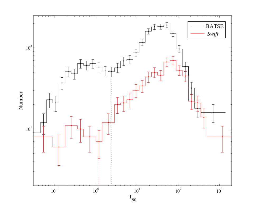
Figure 1: The $log(T_{90})$ double humped durations distributions, $dN/d\log(T_{90})$, of BATSE (black) and Swift (red), binned into equally spaced logarithmic bins. Bins with less than 5 events are merged with their neighbors to reduce statistical errors. The minima in the distributions occur at $T_{90}=2.4\pm 0.4$ sec in the BATSE distribution and at $T_{90}=1.2\pm 0.2$ sec in Swift .

Zhang et al. (2009) suggested to classify individual GRBs using various subsets of properties, e.g. spectral lag, peak energy, etc. These subsets of properties are selected phenomenologically, and are not based on any physical model. The main problem of those classification criteria, which are based on the high-energy emission alone, is that there is a significant overlap, which cannot be quantified, between Collapsars and non-Collapsars in all of them. As a result, the quality of the classification of any of these phenomenological methods cannot be quantified and it is therefore impossible to estimate the fraction of misclassified GRBs. This poses a major problem in using such a method especially since the sample of GRBs with “good data” (afterglow detection, good localization, redshift measurements etc.), is small and very sensitive to misclassification. Other attempts used a statistical approach and tried to evaluate the overlap between the two populations by fitting the distribution of GRBs with two underlying distributions. In this case two lognormal distributions (Horváth 2002; Levesque et al. 2010). The quality of such classification schemes depends entirely on similarity of the true distribution of the two populations to the arbitrarily chosen fitted distribution. Such approach can be trusted only if we know, for example based on physical arguments, what is the underling distribution of at least one of the two populations. Recently, in Bromberg et al. (2011a) we have shown, based on generic physical properties of the Collapsar model, that at short durations the Collapsar distribution is flat. Namely the number of Collapsars per unit duration at short durations is independent of the duration. Building on this result we estimate here the probability that a GRB with a given duration is a Collapsar or not. Not surprisingly this probability depends on the detector and we calculate it for the three major GRB detectors: BATSE, Swift and Fermi GBM. An improved version of this method is obtained by adding a hardness dependence. We present a refined probability distribution that is based on both the duration and the hardness. Needless to say our method is statistical in nature. We cannot determine whether a specific burst is a Collapsar or not, but we can give a probability estimate for this question.

We begin, in section 2, with a discussion of the Collapsars’ duration distribution and an analysis of the observed duration distribution of GRBs . In section 3 we calculate the probability that an observed GRB is a non-Collapsar. Our results imply that short duration Collapsars have been wrongly classified as non-Collapsars, mostly in Swift sample, and this has lead to potential misinterpretation of some of the observed data. In section 4 we discuss the consistency of our findings with some of the recent studies and the implications on the inferred properties of non-Collapsars. We summarize our results and their implications in section 5. We provide a table of the probabilities for each one of the observed Swift bursts with $T_{90}<2$ sec to be a non-Collapsars in an Appendix.

2 The observed GRB duration distribution

Within the Collapsar model a GRB can only be produced after the jet has emerged from the surface of the collapsing star. We (Bromberg et al. 2011a) have recently shown that this leaves a distinctive mark on the observed duration distribution: it is flat at durations shorter than the typical breakout time of the jet from the star (about a few dozen seconds modulo the redshift ). In a nutshell, this result arises from a simple fact. The burst duration is the difference between two quantities: the engine operating time and the jet breakout time. Under quite general conditions the resulting distribution is flat at durations that are shorter than the typical jet breakout time. Indeed, when we plot in fig. (2) the quantity $dN_{GRB}/dT_{90}$ instead of the traditionally shown ${dN_{GRB}}/{d\log(T_{90})}$ (e.g. fig. 1; Kouveliotou et al. 1993) this flat distribution is evident. The plateau appears over about an order of magnitude in duration around a few seconds, in the GRB duration distributions of BATSE, Swift and Fermi GBM, as depicted in fig. 2. The duration is characterized by $T_{90}$ during which 90% of the fluence is accumulated.

At the short end the distribution is rising towards shorter durations. This “bump” in the duration distribution is inconsistent with a Collapsar origin for most of the short duration GRBs. This simple conclusion is consistent with other evidence that a second, non-Collapsar, population of short duration GRBs exists with a different origin than the longer ones. (e.g. Kouveliotou et al. 1993; Barthelmy et al. 2005; Fox et al. 2005; Gehrels et al. 2005; Nakar 2007).

To quantify the non-Collapsars’ duration distribution we make joint fits to the overall duration distributions, including the Collapsar distribution at durations longer than the plateau. Although we are interested only in the short duration regime, where the duration distribution of Collapsars is flat, inclusion of the long end of the distribution is needed to determine the height of the plateau. To test the robustness of our result we fitted various functional forms for the distribution at long durations and verified that the height of the plateaus are consistent within the errors. The results presented here employ a plateau below the typical observed breakout time, $T_{B}$, and a powerlaw with an exponential cutoff above it. For the non-Collapsars we find that the best fitted distribution function is a lognormal. Overall we fit the duration distributions to the function:

$$\frac{dN_{GRB}}{dT_{90}}=A_{NC}\frac{1}{T_{90}\sigma\sqrt{2\pi}}e^{-\frac{(\ln T_{90}-\mu)^{2}}{2\sigma^{2}}}+A_{C}\left\{\begin{array}[]{lc}1&T_{90}\leq T_{B}\\ \left(\frac{T_{90}}{T_{B}}\right)^{\alpha}e^{-\beta(T_{90}-T_{B})}&T_{90}>T_{B},\end{array}\right.$$ (1)

where the first term corresponds to non-Collapsars and the second one to Collapsars.

We consider the data sets of BATSE , Swift , and Fermi GBM . We limit the data to the duration regime of 0-200 sec, which is enough to obtain a good constraint of the plateau hight. We verified that changing this range to 0-1000 sec has no significant effect on our results. We fit each sample with a distribution function according to eq. (1). After using the normalization that the integral of $dN_{GRB}/dT_{90}$ over the duration range equals the number of observed GRBs, we are left with seven free parameters. We obtain good fits with $\chi^{2}$ per degrees of freedom (DOF) of 0.9, 1.3, 1.1 for the BATSE, Swift and Fermi GBM respectively. The corresponding parameters are given in table 1 and Fig. 2 depicts the resulting distribution functions and the data. We find plateaus that extend up to $T_{B}\sim 20$ sec in the BATSE and Fermi GBM durations distributions, and up to $T_{B}\sim 10$ sec in Swift . This is consistent with our expectations from the Collapsar model (Bromberg et al. 2011a).

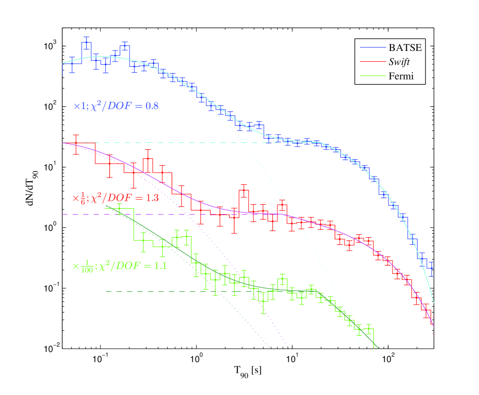
Figure 2: The $T_{90}$ distributions, $dN/dT_{90}$, of BATSE (red), Swift (blue) and Fermi GBM (green) GRBs, binned into equally spaced logarithmic bins. Bins with less than 5 events are merged with their neighbors to get more reliable statistical errors. Note that the quantity $dN/dT$ is depicted and not ${dN}/{d\log(T)}$ as traditionally shown in such plots (e.g., Kouveliotou et al. 1993). The combined best fitted distribution functions of both Collapsars and non-Collapsars are shown with solid lines. The dotted and dashed lines depict the distributions of non-Collapsars and Collapsars respectively in each data set.

Table 1: Best fit parameters

Detector	$A_{NC}$	$\mu$	$\sigma$	$A_{C}$	$T_{B}$ (s)	$\alpha$	$\beta$
BATSE	$545$	$-0.5\pm 0.1$	$1.32\pm 0.07$	$25.5^{+1.9}_{-1.4}$	$19.4^{+2.5}_{-4.2}$	$-0.33\pm 0.2$	$0.019\pm 0.003$
Swift	$42$	$-1.5\pm 0.5$	$1.5\pm 0.4$	$10.0\pm 2.3$	$7.9\pm 3.5$	$-0.3\pm 0.2$	$0.01\pm 0.003$
Fermi GBM	$128$	$-1.5\pm 0.6$	$1.9\pm 0.4$	$8.8\pm 0.2$	$18.2^{+1.3}_{-11.6}$	$-1.2\pm 0.36$	$0.008\pm 0.001$

3 The non-Collapsars probability function

The probability that a GRB with a given $T_{90}$ is a non-Collapsar is given by the fraction of non-Collapsars within the observed GRBs at a given duration:

$$f(T_{90})=A_{NC}\frac{1}{T_{90}\sigma\sqrt{2\pi}}e^{-\frac{(\ln T_{90}-\mu)^{2}}{2\sigma^{2}}}\left(\frac{dN_{GRB}}{dT_{90}}\right)^{-1},$$ (2)

where $dN_{GRB}/dT_{90}$ is given by eq. (1). To estimate the errors in $f_{NC}$ we simulate, for each one of the samples, distributions of $T_{90}$ drawn randomly from the best fitted distribution function $dN_{GRB}/dT_{90}$. We then bin the simulated data sets, and repeat the process of parameter fitting using eq.(1) to obtain $f_{NC}$ . We repeat this processes $1000$ times and look for the ranges of $f_{NC}$ that encompasses $68\%$ of the cases. Fig. 3 depicts $f_{NC}$ $(T_{90})$ for the BATSE, Swift and Fermi GBM samples. The solid lines depict $f_{NC}$ , calculated from the observed data, and the blue region describes the $1\sigma$ error estimate. Table 1 lists the $T_{90}$ values that correspond to some selected probabilities for the three detectors.

These results clearly show that the choice of $T_{90}=2$ sec as a threshold to identify non-Collapsars is suitable for BATSE, and possibly also for Fermi GBM. A BATSE (Fermi GBM) burst with $T_{90}=2$ sec has a probability $>70\%$ ($\gtrsim 40\%$) to be a non-Collapsar. However, the probability of a similar Swift burst to be a non-Collapsar is only $0.16\pm 0.14$. It is most likely a Collapsar! The level of false identification, for a given duration threshold, $T_{th}$ can be seen in Fig. 4 that depicts the integrated fraction of Collapsars (out of the total number of GRBs) with duration $T_{90}\leqslant T_{th}$. The total number of Collapsars with duration $T_{90}<2$ sec in the Swift sample is estimated to be $19\pm 5$ out of 53 GRBs. Thus, an arbitrary Swift sample selected with the $T_{th}=2$ sec criterion contains about than 40% Collapsars that have been misclassified as non-Collapsars. This should be compared with about 10% and 15% of misclassified Collapsars in the corresponding BATSE and Fermi samples (see fig. 4) with the same $T_{th}$. The criterion $T_{th}=2$ sec for selecting non-Collapsars in Swift is simply very bad for most studies of non-Collapsars.

Any single criteria that should distinguish according to the durations between Collapsars and non-Collapsars should be detector dependent. A longer $T_{th}$ increases the size of the SGRBs sample (that are supposedly non-Collapsars) but it increases at the same time the number of misidentified Collapsars in the sample. A shorter threshold yields smaller but cleaner samples. The specific choice of $T_{th}$ should be considered for each study, balancing the need of a large sample with the importance of purity. A reasonable choice that should be adequate to many studies is choosing the threshold probability as $f_{NC}$ $=0.5$. This reconciles between these conflicting requirements and allows us to classify both Collapsars and non-Collapsars with a single criterion. Adopting this probability we find that the corresponding $T_{90}$ threshold values are: $T_{th}=0.8\pm 0.3$ sec for Swift , $T_{th}=1.7^{+0.4}_{-0.6}$ sec for Fermi GBM and $T_{th}=3.1\pm 0.5$ sec for BATSE. The total number of misclassified Collapsars in samples selected according to these criteria constitute about 20% of the Swift samples and $\sim 14\%$ of the BATSE and Fermi GBM samples (fig. 4).

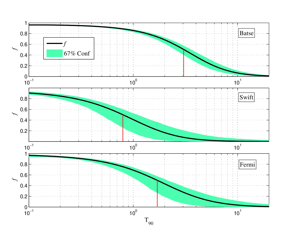
Figure 3: The fraction $f_{NC}$ of non-Collapsars as a function of $T_{90}$ for BATSE, Swift & Fermi GBM (from top to bottom). This fraction represents the probability that a GRB with an observed duration $T_{90}$ is a non-Collapsars. The shaded regions represent the 68% confidence range. The red vertical lines mark the values of $T_{90}$ where $f_{NC}$ $=0.5$ (See table 2 for numeric values of $T_{90}$ that correspond to some selected $f_{NC}$ values).

Table 2: The $T_{90}$ (sec) that corresponds to some selected $f_{NC}$ values in the three satellites

	$f_{NC}$	0.9	0.8	0.7	0.6	0.5	0.4	0.3
Satellite
BATSE		$0.7^{+0.1}_{-0.1}$	$1.4^{+0.2}_{-0.2}$	$1.9^{+0.3}_{-0.3}$	$2.5^{+0.4}_{-0.4}$	${\bf 3.1^{+0.5}_{-0.5}}$	$3.8^{+0.7}_{-0.7}$	$4.7^{+0.9}_{-0.9}$
Swift		$0.11^{+0.05}_{-0.11}$	$0.3^{+0.1}_{-0.1}$	$0.4^{+0.1}_{-0.1}$	$0.6^{+0.2}_{-0.2}$	${\bf 0.8^{+0.3}_{-0.3}}$	$1.0^{+0.5}_{-0.4}$	$1.3^{+0.7}_{-0.6}$
Fermi GBM		$0.3^{+0.1}_{-0.2}$	$0.7^{+0.1}_{-0.2}$	$1.0^{+0.2}_{-0.3}$	$1.3^{+0.3}_{-0.4}$	${\bf 1.7^{+0.4}_{-0.6}}$	$2.2^{+0.7}_{-0.9}$	$2.8^{+1.1}_{-1.2}$

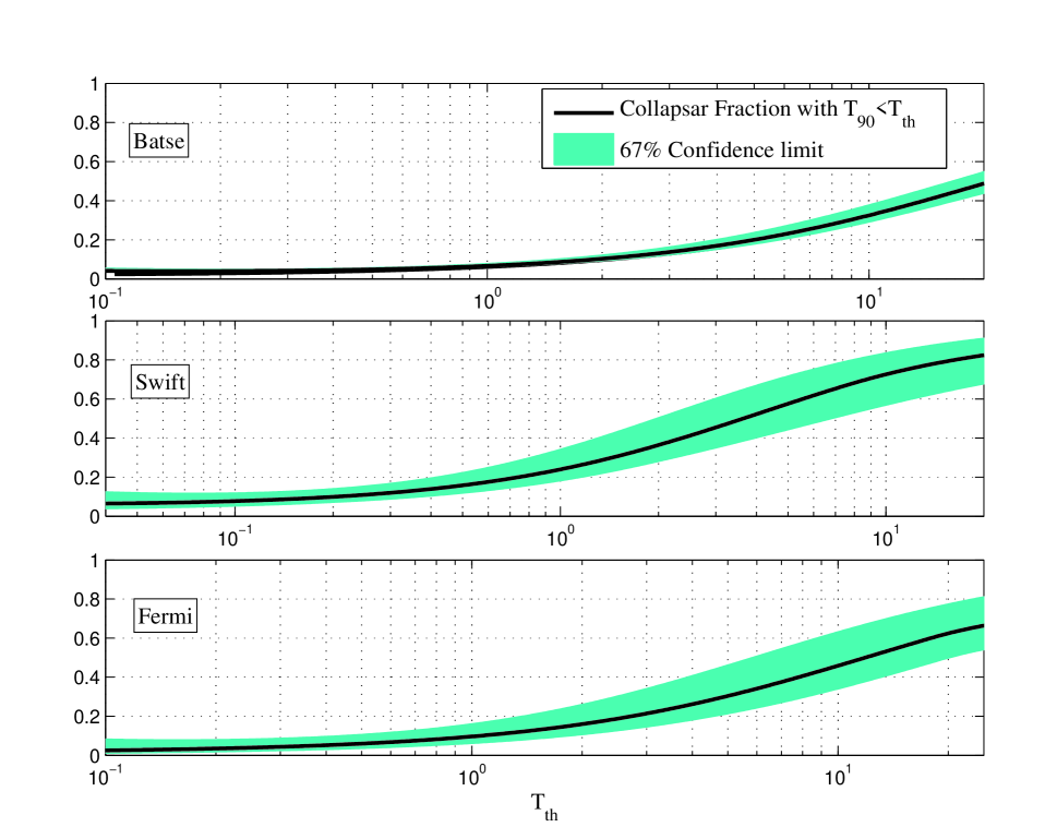
Figure 4: The integrated fraction of Collapsars with duration $T_{90}\leqslant T_{th}$, for BATSE, Swift & Fermi GBM (from top to bottom). This is the fraction of Collapsars that are misclassified as non-Collapsars with durations shorter that the threshold, $T_{th}$. The shaded regions represent the 68% confidence limits.

3.1 The non-Collapsar probability as a function of duration and hardness

As already mentioned short GRBs are harder on average than long ones (Kouveliotou et al. 1993). It is natural to expect that the ratio of non-Collapsars to Collapsars and the probability function, $f_{NC}$ , should increase with the GRB hardness. Therefore the combination of duration and hardness provides a stronger way to distinguish between non-Collapsars and Collapsars. To examine the duration-hardness probability we divide the samples into three hardness subgroups: soft, intermediate and hard, and preform the same analysis on each subgroups: We fit a duration distribution function and calculate the probability function, $f_{NC}$ , and its $1\sigma$ variance. We consider two hardness thresholds: The soft and intermediate subgroups are separated by the average hardness of Collapsars which we estimate using GRBs with $T_{90}>20$ sec, where the contribution of non-Collapsars in all samples is negligible. The intermediate and hard subgroups are separated by the average hardness of non-Collapsars which is estimated using GRBs with $T_{90}<0.5$ sec. The spectral hardness of different satellite samples is quantified differently for each detector, depending on the available information for each database. For BATSE we use the hardness ratio parameter, HR₃₂, defined as the ratio between the photon counts in energy channel 3 (100 - 300 keV) and energy channel 2 (50 - 100 keV). In Swift and Fermi GBM samples we use the powerlaw index (PL) of the observed spectrum obtained by fitting a single powerlaw in the energy range $15-150$ keV (Swift ) or $10-2000$ keV (Fermi). Note that in the Swift sample, only $\sim 87\%$ of the GRBs have a spectral fit to a single power-law. The spectrum of the other $13\%$ is fitted with a powerlaw+exponential cutoff, and we omit these bursts from this analysis.

$\begin{array}[]{c}\begin{array}[]{cc}\includegraphics[width=231.26378pt]{hardness_batse-paper.eps}&\includegraphics[width=231.26378pt]{Swift_PhotonInd_PL_T90-paper-binning-5.eps}\end{array}\\ \includegraphics[width=231.26378pt]{Fermi_PhotonInd_PL_T90-paper-binning-5.eps}\end{array}$

Figure 5: The hardness ratio of BATSE GRBs (top left) and the powerlaw index of Swift GRBs (top right) and Fermi GRBs (bottom) as a function of $T_{90}$.

If the distribution functions of Collapsars and non-Collapsars don’t depend strongly on the spectral hardness, then varying the hardness threshold would only change the relative ratio of Collapsars to non-Collapsars, while the overall shape of the duration distribution functions of the two populations would remain unchanged. To examine this we fit each hardness subgroup with the same distribution function as in the full sample of the corresponding detector. We only rescale $A_{NC}$ and $A_{C}$ according to the number of non-Collapsars and Collapsars in the subgroup relative to their number in the full sample. We evaluate the ratio of non-Collapsars by dividing the number of GRBs with $T_{90}<0.5$ sec in the subgroup with their number in the full sample. The ratio of Collapsars is evaluated in a similar way using GRBs with $T_{90}>20$ sec. We find good fits in all hardness subgroups with $\chi^{2}/dof$ of $\sim 0.8-1.8$. This good fit indicates a weak dependency of the duration distributions of Collapsars and non-Collapsars on the hardness.

Figure 6 depicts the observed duration distributions of the three hardness subgroups of each detector. The harder subgroups have more prominent ’bumps’ at short durations together with relatively lower plateaus that become visible only at longer durations. This is the expected behavior if the fraction of non-Collapsars increases with the GRB hardness. The $dN/dT_{90}$ distributions and their $\chi^{2}/DOF$ values are shown in fig. 6. The resulting probability functions of each subgroup are shown in figs. 7-9. In table 3 we list the $T_{90}$ values that correspond to specific values of $f_{NC}$ in each subgroup. In the hard BATSE subgroup non-Collapsars dominate the distributions up to $T_{90}=7.8^{+1.4}_{-1.0}$ sec, while in the hard Swift and Fermi GBM samples non-Collapsars dominate up to $T_{90}=2.8^{+1.5}_{-1.0}$ and $T_{90}=5.4^{+3.9}_{-2.0}$ sec respectively. The transition between Collapsars and non-Collapsars in the intermediate subgroups roughly follow the same values as in the complete samples: $T_{90}=2.9\pm 0.4$, $T_{90}=0.6^{+0.2}_{-0.3}$ and $T_{90}=1.6^{+0.8}_{-0.6}$ sec for BATSE, Swift and Fermi GBM respectively. In the soft subgroups non-Collapsars dominate only up to $T_{90}=1.1^{+0.2}_{-0.3}$ sec in BATSE, $T_{90}=0.3^{+0.4}_{-0.2}$ sec in Swift , and up to $T_{90}=0.6^{+0.6}_{-0.3}$ sec in Fermi GBM.

$\begin{array}[]{c}\begin{array}[]{cc}\includegraphics[width=252.94499pt]{dNdT_renormalized_BATSE_fit-paper-binning-5-0-fit.eps}&\includegraphics[width=252.94499pt]{dNdT_renormalized_Swift_PL_Index_Batse-paper-binning-5-0-fit.eps}\end{array}\\ \includegraphics[width=252.94499pt]{dNdT_renormalized_Fermi_PL_Index-paper-binning-5-0-fit.eps}\end{array}$

Figure 6: $dN/dT_{90}$, of the three hardness subgroups of the BATSE (upper left) Swift (upper right) and Fermi GBM (lower) samples, binned into equally spaced logarithmic bins. Bins with less than 5 events are merged with their neighbors to reduce statistical errors. The best fitted joined distribution functions are marked with solid lines.

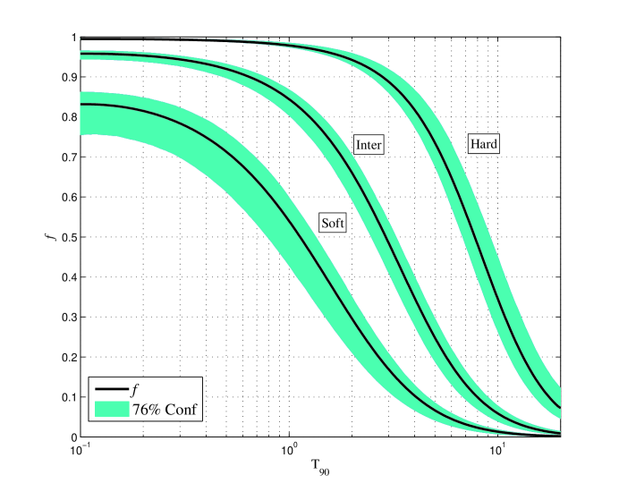
Figure 7: The fraction, $f_{NC}$ , of non-Collapsars as a function of the observed duration, $T_{90}$, in the 3 hardness subgroups of BATSE.

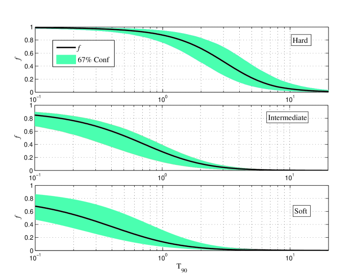
Figure 8: Same as fig. 7 for Swift

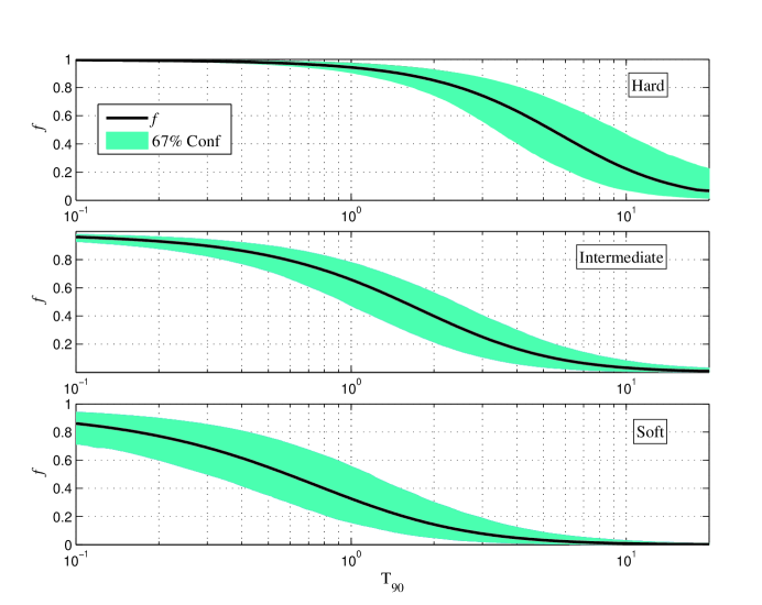
Figure 9: Same as fig. 7 for Fermi GBM

Table 3: The $T_{90}$ (s) at different $f_{NC}$ in the three hardness subgroups for each satellite.

		0.9	0.8	0.7	0.6	0.5	0.4	0.3
BATSE	Hard (HR${}_{32}>5.5$)	$2.8^{+0.6}_{-0.3}$	$4.2^{+0.8}_{-0.5}$	$5.4^{+1.0}_{-0.6}$	$6.6^{+1.2}_{-0.8}$	${\bf 7.8^{+1.4}_{-1.0}}$	$9.1^{+1.7}_{-1.2}$	$10.8^{+2.1}_{-1.4}$
	Intermediate ($5.5>$HR${}_{32}>2.6$)	$0.6^{+0.1}_{-0.2}$	$1.3^{+0.2}_{-0.2}$	$1.8^{+0.2}_{-0.3}$	$2.3^{+0.3}_{-0.4}$	${\bf 2.9^{+0.4}_{-0.4}}$	$3.6^{+0.4}_{-0.5}$	$4.4^{+0.5}_{-0.6}$
	Soft ($2.6>$HR32)	…	$0.2^{+0.2}_{-0.2}$	$0.5^{+0.2}_{-0.3}$	$0.8^{+0.2}_{-0.3}$	${\bf 1.1^{+0.2}_{-0.3}}$	$1.5^{+0.3}_{-0.4}$	$2.0^{+0.3}_{-0.5}$
Swift	Hard (PL$>-1.13$)	$0.9^{+0.6}_{-0.4}$	$1.4^{+0.9}_{-0.5}$	$1.9^{+1.1}_{-0.6}$	$2.3^{+1.3}_{-0.8}$	${\bf 2.8^{+1.5}_{-1.0}}$	$3.4^{+1.9}_{-1.1}$	$4.2^{+2.2}_{-1.4}$
	Intermediate ($-1.13>$PL$>-1.65$)	$0^{+0.09}$	$0.16^{+0.09}_{-0.16}$	$0.3^{+0.1}_{-0.2}$	$0.4^{+0.2}_{-0.2}$	${\bf 0.6^{+0.2}_{-0.3}}$	$0.7^{+0.2}_{-0.4}$	$1.0^{+0.3}_{-0.5}$
	Soft ($-1.65>$PL)	$0^{+0.05}$	$0^{+0.18}$	$0.09^{+0.22}_{-0.09}$	$0.16^{+0.28}_{-0.16}$	${\bf 0.3^{+0.4}_{-0.2}}$	$0.4^{+0.4}_{-0.2}$	$0.5^{+0.5}_{-0.3}$
Fermi GBM	Hard (PL$>-1.34$)	$1.5^{+1.0}_{-0.5}$	$2.5^{+1.6}_{-0.8}$	$3.4^{+2.2}_{-1.1}$	$4.3^{+3.0}_{-1.5}$	${\bf 5.4^{+3.9}_{-2.0}}$	$6.6^{+5.1}_{-2.5}$	$8.2^{+7.1}_{-3.3}$
	Intermediate ($-1.32>$PL$>-1.52$)	$0.3^{+0.2}_{-0.2}$	$0.6^{+0.3}_{-0.2}$	$0.9^{+0.5}_{-0.3}$	$1.2^{+0.6}_{-0.5}$	${\bf 1.6^{+0.8}_{-0.6}}$	$2.0^{+1.0}_{-0.8}$	$2.6^{+1.4}_{-1.0}$
	Soft ($-1.52>$PL)	$0.06^{+0.14}_{-0.06}$	$0.17^{+0.25}_{-0.17}$	$0.3^{+0.4}_{-0.2}$	$0.4^{+0.5}_{-0.2}$	${\bf 0.6^{+0.6}_{-0.3}}$	$0.8^{+0.7}_{-0.4}$	$1.1^{+0.9}_{-0.5}$

The probability functions we obtained here can be used to classify the GRBs detected by BATSE, Swift and Fermi GBM according to their duration and hardness. For GRBs that cannot be assigned to one of those hardness subgroups (e.g the 13% of Swift GRBs whose spectra are fitted with a powerlaw+exponential cutoff) the classification can be done using the overall probability function of the complete Swift sample. For GRBs that have been detected by HETE and Integral we recall that the spectral window observed by HETE is $8-500$ keV, which is closer to the Swift /BAT while Integral, on the other hand, observes at a spectral range of 15 keV - 10 MeV, which is closer to BATSE’s range. As a first approximation one can use the corresponding $f_{NC}$ values of these detectors.

In Appendix A we collect all Swift GRBs with $T_{90}<2$ observed to date. The table includes also GRBs with a hard short spike plus a soft extended emission and a number of other GRBs with duration $>2$ sec that are sometimes considered as possible non-Collapsars. For each GRB we calculate the probability to be a non-Collapsar from the duration and power-law index ,$f_{NC}$ $(T_{90},PL)$. For those GRBs with a spectral fit of a powerlaw+exponential cutoff, we calculate the probability to be a non-Collapsar from the duration alone, $f_{NC}$ $(T_{90})$. Important GRBs are emphasized with bold text. The table also includes a few important GRBs detected by HETE or Integral. For these GRBs we estimate $f_{NC}$ $(T_{90})$ using the probability functions of Swift and BATSE respectively. This table can be used to evaluate the contamination by Collapsars in present samples of SGRBs and to select low contamination samples in future studies.

4 Consistency checks with studies of contaminated samples

The commonly used criterion to distinguish Collapsars from non-Collapsars is the duration ($T_{90}\gtrless 2$ sec). This criterion is applied to GRBs that are detected by all $\gamma$-ray satellites including Swift , that supplies the largest number of well localized short duration GRBs. As we have shown earlier Swift GRBs with $T_{90}>0.8$ sec have high probability to be Collapsars. This could have led to a “Collapsar contamination” in current Swift samples of SGRBs that are based on the 2 sec criterion, and might have affected the results of studies based on these samples. Interestingly such studies (e.g. Berger 2009, 2011), have shown that the environments of SGRBs are different than the environments of LGRBs. Whereas LGRBs are associated with intensive star formation, arise in low metallically irregular star forming galaxies (see however Levesque et al. 2010b, c; Savaglio et al. 2012, for examples of high metalicity LGRB hosts) and are concentrated towards star forming regions in their galaxies. SGRBs are associated with a broad distribution of galaxy types and arise in hosts with a broad range of star formation rate and metallicities and show a larger scatter in the distance distribution from their hosts’ centers. One may wonder how these results are consistent with our claim that the 2 sec classification is not valid for the Swift sample.

Table 4 lists the GRBs and the host galaxy characteristics used in the Berger (2009, 2011) sample. It also includes the probability that the associated SGRB are non-Collapsars (based the combination of duration and power-law index). In addition to eight ‘classically selected’ SGRBs ($T_{90}<2$ sec) this sample includes also four GRBs with $T_{90}>2$ sec. These GRBs are characterized by a short hard initial spike followed by a long tail of softer emission. They are often considered as non-Collapsars since their initial spikes resemble a classical SGRB (see Nakar 2007). However, since the overall duration is not well defined our classification scheme cannot attribute a non-Collapsar probability to these bursts.

Even though our probabilistic approach is incapable of determining whether a specific burst is a Collapsar or not, a clear picture emerges from table 4. Four out of eight classifiable bursts are non-Collapsars at very high probabilities. Two bursts are almost certainly Collapsars while the last two are marginal: the probability of each one of those two to be a Collapsar is larger than 60%, however the probability that both are Collapsars is less than 50%. These fractions are consistent with what is expected, according to our analysis, from a Swift sample with a 2 sec criteria for which $\sim 60\%$ of the bursts should be non-Collapsars and the rest Collapsars.

Within the sub-sample of four non-Collapsars we observe a large spread in SFRs, in specific SFRs and in galactic luminosities. Distances from the center of the host have typically large observational error, but at least one is quite far from the center ($\sim 44^{+12}_{-23}$ kpc). There is not enough data to determine the metallicity. These results show a large spread in the observed quantities, in a large contrast with the rather narrowly distributed host properties of LGRBs (Collapsars). This is similar to the conclusion of Berger (2009, 2011). It demonstrates that also when a less contaminated, but smaller, sample is examined non-Collapsars hosts have a different distribution than Collapsar hosts and consequently that the two populations have different progenitors. On the other hand, as expected, the properties of the hosts of the two Collapsar candidates are fully consistent with those of typical LGRB hosts. Finally, the properties of the hosts of the two bursts with marginal classification are also consistent with being either Collapsar or non-Collapsar hosts.

The conclusion that the properties of the non-Collapsars’ hosts are widely distributed whereas those of the Collapsars’ hosts are narrowly distributed implies that our classification is consistent with the results of Berger (2009, 2011) even though the latter are based of a significantly contaminated sample. A wide distribution contaminated by a narrowly distributed population retains it basic feature of a wide distribution, and this is what happens here. The non-Collapsars within the Berger (2009, 2011) SGRB sample are numerous enough to result in a wide distribution that is significantly different from the one of Collapsars. However, while our conclusions are in line with the basic results of Berger (2009, 2011), the details of the distribution, such as the ratio of high SFR to low SFR hosts or the distribution of distances from center, are influenced by the contamination and a quantitative study of the distribution of the host properties should take this factor into account.

The possible effects of contaminating Collapsars on studies of properties of SGRBs vary from one study to another. Different samples have different contaminations and different properties are influenced differently. The probabilities given in appendix A can be used to evaluate the likelihood that different bursts are non-Collapsars or Collapsars and with these to estimate the quality of a specific sample and the significance of results based on this sample. In general one should proceed with care before adopting simply the results of a study of an SGRB sample as reflecting the properties of non-Collapsars. In this context it is interesting to mention a few GRBs that play a major role in the current view of non-Collapsar properties. GRB 060121 and GRB 090426 are two SGRBs with a secure host at redshift $\geqslant 2$ that have led to the suggestion of a high redshift non-Collapsar population. GRB 100424A has a redshift of $z=1.288$. All other SGRBs with secure redshift are at $z\leqslant 1$. We find that the probabilities that these bursts are non-Collapsars are $0.17^{+0.14}_{-0.15}$, $0.10^{+0.15}_{-0.06}$ and $0.08^{+0.12}_{-0.04}$ for GRBs 060121, 090426 and 100424A respectively. Surely, one cannot establish a new population of high redshift non-Collapsars based on these events. Another pivotal burst is 051221A; the only SGRB to date with a clear simultaneous optical/X-ray break in its afterglow, which is used to measure its beaming (Soderberg et al. 2006; Burrows et al. 2006). We find that the probability that GRB 051221A is a non-Collapsar is $0.18^{+0.08}_{-0.11}$. This highlights our ignorance of the collimation (if there is any) of non-Collapsar outflows. It also highlights the fact that no firm conclusion can be drawn on non-Collapsars based on a single burst that is classified using its high energy emission properties alone.

Table 4: The sample of Berger (2009, 2011) SGRBs.

GRB	$T_{90}$	PL	$f_{NC}$ a	$L_{b}$	SFR	SFR/$L_{b}$	12+log(O/H)∗	offset	ref
	(s)			($L_{*}$)	($M_{\odot}/yr$)	($M_{\odot}/yr\cdot L_{*}$)		(kpc)
050709b	0.07		$0.92^{+0.02}_{-0.03}$	0.1	0.2	2	8.5	3.8	1,2
061217	0.210	$0.86\pm 0.30$	$1^{+0.00}_{-0.21}$	0.4	2.5	6.25		$0-30$	1,3
050509B	0.073	$1.57\pm 0.38$	$0.87^{+0.04}_{-0.16}$	5	$<0.1$	$<0.02$		$44^{+12}_{-23}$	1,2
060801	0.490	$0.47\pm 0.24$	$0.95^{+0.03}_{-0.05}$	0.6	6.1	10.17		$19\pm 16$	1,3
070724A	0.400	$1.81\pm 0.33$	$0.37^{+0.26}_{-0.17}$	1.4	2.5	1.79	8.9	$4.8\pm 0.1$	1,4
070429B	0.470	$1.72\pm 0.23$	$0.32^{+0.26}_{-0.15}$	0.6	1.1	1.83		$40^{+48}_{-40}$	1,3
051221A	1.400	$1.39\pm 0.06$	$0.18^{+0.08}_{-0.11}$	0.3	1	3.33	8.2 or 8.7	$0.8\pm 0.3$	1,5
060121b	1.97		$0.17^{+0.14}_{-0.15}$		1			$\sim 1$	1,3
050724	3(96)†			1	$<0.05$	$<0.05$		2.6	1,2
061006	$~{}0.5(123)^{\dagger}$			0.1	0.2	2	8.6	$1.3$	1,3
061210	0.2(85)†			0.9	1.2	1.33	8.8	$11\pm 10$	1,3
070714B	3(64)†			0.1	0.4	4		$\lesssim 4$	1,3
a Swift GRBs with a single power-law spectral fit are assigned a probability $f_{NC}$ $(T_{90},PL)$.
Other GRBs can only be assigned a probability $f_{NC}$ $(T_{90})$.
b A GRB detected by HETE, $f_{NC}$ $(T_{90})$ is estimated using Swift probability function.
${\dagger}$ GRB with an extended softer emission
∗ The metallicity is measured by the ratio of Oxygen to Hydrogen lines. The range of values
of $8.2-8.9$ shown in the table corresponds to $\sim 0.3-1.6Z_{\odot}$.
References: 1) Berger (2009); 2) Fox et al. (2005); 3) Fong, Berger, & Fox (2010);
4) Berger et al. (2009); 5) Soderberg et al. (2006)

5 Summary

GRBs are widely classified as long and short, according to their duration $T_{90}\lessgtr 2$ sec, based on the general belief that this observational classification is associated with a physical one and that the two populations have different origins: long GRBs are Collapsars and short ones are non-Collapsars (possibly arising from neutron star mergers, but at present, this association is still uncertain). This classification scheme is known to be imperfect due to the large overlap in the duration distribution between the two populations. It is also used for all detectors, although it is known that any classification scheme depends on the detector (e.g., Nakar 2007). The problem with this method is that, first it is impossible to know how trustable are results that are based on a single classified event. Second, the level of contamination in any studied sample is unknown. The main reason for this flawed practice is simply the lack of a reliable and quantifiable classification scheme. This is what we provide in this paper. Based on a physically motivated model we have shown in an earlier study (Bromberg et al. 2011a) that at short durations the Collapsar distribution is flat, up to a typical duration of $\sim 20$ sec. This enables us to recover the non-Collapsar distribution from the overall duration distribution and to assign probability that a burst with a given duration and hardness is a non-Collapsar.

We carry out this analysis for three major GRB satellites, BATSE, Fermi and Swift . We first find the probability that a burst is a non-Collapsar based on its duration alone, $f_{NC}$ $(T_{90})$. We find that it depends strongly on the observing satellite and in particular on its spectral window. For a given duration the probability that a BATSE burst is a non-Collapsar is larger than the probability that a Swift burst is a non-Collapsar. A useful threshold duration that separates Collapsars from non-Collapsars is that where $f_{NC}$ $(T_{90})=0.5$. We find that it is $T_{90}=3.1\pm 0.5$ sec in BATSE, $T_{90}=1.7^{+0.4}_{-0.6}$ sec in Fermi GBM and $T_{90}=0.8\pm 0.3$ sec in Swift.

As short GRBs are harder on average than long ones (Kouveliotou et al. 1993), it is natural to expect that GRBs with a hard spectrum have a higher probability to be non-Collapsars than softer ones. Thus, a better classification can be achieved by considering the hardness, in addition to the duration. We separate the sample of each satellite to three sub-samples based on the bursts hardness and repeat the analysis. Not surprisingly there are fewer non-Collapsars in the soft subgroups and more in the harder ones. Interestingly the duration distributions of both Collapsars and non-Collapsars depend only weakly on the hardness and only the relative normalization between the two groups varies as we consider subgroups of different hardness. As there are more non-Collapsars in the hard subgroups, non-Collapsars dominate in these subgroups even at relatively long durations. For example In the hard BATSE subgroup the probability, $f_{NC}$ , that a burst is a non-Collapsar remains $>0.5$ up to durations $T_{90}\simeq 8$ sec. In the hard Fermi GBM and Swift subgroups $f_{NC}$ $>0.5$ up to $\simeq 5$ and $\simeq 3$ sec respectively. A soft GRB, on the other hand, is more likely to be a Collapsar. In this case $f_{NC}$ $>0.5$ up to $T_{90}\simeq 1$ sec for BATSE’s soft subgroup, up to $T_{90}\simeq 0.6$ sec in Fermi GBM and only up to $T_{90}\simeq 0.3$ in Swift ’s subgroups. These values should replace the average values as dividing durations between Collapsars and non-Collapsars, whenever hardness information is available. In particular for Swift , $2.8^{+1.5}_{-1.0}$, $0.6^{+0.2}_{-0.3}$, and $0.3^{+0.4}_{-0.2}$ sec should replace the value of $0.8\pm 0.3$ sec for the hard, intermediate and soft subgroups respectively. Our results well agree with the overall behavior seen when comparing different satellites. Swift ’s window is much softer than BATSE’s and Fermi’s and the transition in Swift ’s overall sample between non-Collapsars and Collapsars occurs at shorter durations relative to the other satellites. This is a general pattern seen in both the overall sample and in the hardness subgroups.

We find that the transition between Collapsars and non-Collapsars is not sharp and that there is a large overlapping region where both Collapsars and non-Collapsars co-exist. There are short durations Collapsars with durations shorter than 1 sec as well as non-Collapsars at observed durations as long as 10 sec. The traditional method to divide bursts to “long” and “short” according to a sharp observed duration criteria: $T_{90}\lessgtr 2$, introduces both “false positive” and “false negatives” when we interpret duration as a proxy for a different physical origin. The choice of the division criteria should depend on the detector’s observing windows but it should also depend on our tolerance for contamination by “falsely” classified bursts. When interested in Collapsars, the solution is trivial. Choosing a conservative large duration will eliminate a few short duration Collapsars but will results in a sample containing practically only Collapsars. The small number of short duration bursts makes it difficult to adopt a similar conservative policy for them and the classification criterion should be chosen carefully in each study. Finally, our results show clearly that no high significance result concerning non-Collapsars can be derived based on a single burst, which is classified according to its high energy properties alone.

Next we examine the implication of the currently used criterion $T_{90}\lessgtr 2$ on the different satellite samples. It is conservative for BATSE, where Only 10% of bursts that are shorter than 2 sec are Collapsars. One can consider a BATSE ($T_{90}\leq 2$ sec) sample as reasonably free of false positives. The corresponding fraction of “false positives” for Fermi is higher (20%) but still acceptable for many purposes. However this criteria is not good for Swift . About 40% of Swift bursts with $T_{90}<2$ sec, that have been traditionally classified and studied as SGRBs are Collapsars. Thus the standard and commonly use sample of Swift GRBs with $T_{90}\lessgtr 2$ sec which is the source of the only sample of well localized short GRBs is heavily contaminated with Collapsars! This must have influenced the results of non-Collapsars studies that are based on Swift GRBs. Interestingly, this Collapsar contamination didn’t affect qualitatively the main conclusion concerning non-Collapsar hosts (Berger 2009, 2011), namely the observation that these hosts have a wide distributions of SFR, luminosities and metallicities and that the conclusion that the positions of non-Collapsars has a wide spread within the host galaxy. Such distributions are significantly different than those of Collapsar’s host. However, quantitative features of these distributions must have been distorted.

While the complete implications of our results on studies of non-Collapsars is beyond the scope of this work, there are three important points that stand out. (i) There is no convincing evidence for high redshift non-Collapsars. All the bursts with secure redshift that are non-Collapsars at high probability are at $z<1$. (ii) There is no convincing evidence for beaming in non-Collapsars. GRB 051221A is the only SGRB that show a multi-wavelength afterglow break, that is interpreted as a jet break and is considered as the strongest evidence for beaming in non-Collapsars. However, our results show that the probability that this burst is indeed a non-Collapsar is only $0.18^{+0.08}_{-0.11}$. Apparently, non-Collapsars may or may not be beamed as far as we currently know. (iii) The duration of a non-negligible fraction of the non-Collapsars is $10$ s and even longer. This implies (under most GRB models) that the central engine of these events works continuously in the mode that produces the initial hard GRB emission for that long. This fact should be accommodated by any model of non-Collapsar central engine.

This research is supported by an ERC advanced research grant, by the Israeli Center for Excellence for High Energy AstroPhysics (T.P.), by ERC and IRG grants, and a Packard, Guggenheim and Radcliffe fellowships (R.S.), and by ERC starting grant and ISF grant no. 174/08 (E.N.)

Appendix A Swift SGRBs

GRB	$T_{90}[s]$	PL	$f_{NC}$ a	z	Ref
050202	0.270	$1.44\pm 0.32$	$0.71^{+0.27}_{-0.23}$
050509B	0.073	$1.57\pm 0.38$	$0.87^{+0.04}_{-0.16}$	0.225	1
050709b	0.07		${0.92^{+0.02}_{-0.03}}$	0.161	2
050724	3(96)†			0.257	3
050813	0.450	$1.28\pm 0.37$	$0.57^{+0.39}_{-0.24}$	0.722∗	4
050906	0.258	$2.46\pm 0.43$	$0.49^{+0.25}_{-0.20}$
050925	0.070	….d….	$0.92^{+0.02}_{-0.03}$
051105A	0.093	$1.22\pm 0.30$	$0.85^{+0.14}_{-0.17}$
051210	1.300	$1.06\pm 0.28$	$0.82^{+0.10}_{-0.61}$
051221A	1.400	$1.39\pm 0.06$	$0.18^{+0.08}_{-0.11}$	0.546	5
060121b	1.97		${0.17^{+0.14}_{-0.15}}$	$1.7\leqslant z\leqslant 4.5$	6
060313	0.740	$0.70\pm 0.07$	$0.92^{+0.05}_{-0.08}$
060502B	0.131	$0.98\pm 0.19$	$0.99^{+0.01}_{-0.16}$	0.287	7
060505	4.000	$1.29\pm 0.28$	$0.03^{+0.29}_{-0.02}$	0.089	8
060614	6(108)†			0.125	9
060801	0.490	$0.47\pm 0.24$	$0.95^{+0.03}_{-0.05}$	1.131∗	10
061006	0.5(123)†			0.438	11
061201	0.760	$0.81\pm 0.15$	$0.92^{+0.05}_{-0.08}$	0.11 / 0.087∗	12
061210	0.192(85)†			0.410∗	13
061217	0.210	$0.86\pm 0.30$	$0.98^{+0.01}_{-0.23}$	0.827	14
070209	0.090	$1.00\pm 0.38$	$0.99^{+0.01}_{-0.13}$
070406	1.200	$1.38\pm 0.60$	$0.23^{+0.61}_{-0.13}$
070429B	0.470	$1.72\pm 0.23$	$0.32^{+0.26}_{-0.15}$	0.904	15
070707c	1.1		${0.84^{+0.02}_{-0.03}}$
070714A	2.000	$2.60\pm 0.20$	$0.04^{+0.07}_{-0.02}$
070714B	3(64)†			0.92	16
070724A	0.400	$1.81\pm 0.33$	$0.37^{+0.26}_{-0.17}$	0.457	17
070729	0.900	$0.96\pm 0.27$	$0.89^{+0.06}_{-0.57}$
070809	1.300	$1.69\pm 0.22$	$0.09^{+0.13}_{-0.05}$
070810B	0.080	$1.44\pm 0.37$	$0.86^{+0.13}_{-0.16}$
070923	0.050	$1.02\pm 0.29$	$0.99^{+0.00}_{-0.11}$
071112B	0.300	$0.69\pm 0.34$	$0.97^{+0.01}_{-0.03}$
071227	1.800	$0.99\pm 0.22$	$0.71^{+0.15}_{-0.59}$	0.384	18
080121	0.700	$2.60\pm 0.80$	$0.21^{+0.23}_{-0.11}$
080123	0.8(115)†
080426	1.700	$1.98\pm 0.13$	$0.06^{+0.09}_{-0.03}$
080702A	0.500	$1.34\pm 0.42$	$0.53^{+0.42}_{-0.23}$
080905A	1.000	$0.85\pm 0.24$	$0.88^{+0.07}_{-0.11}$	0.122	19

GRB	$T_{90}[s]$	PL	$f_{NC}$ a	z	Ref
080919	0.600	$1.10\pm 0.26$	$0.94^{+0.03}_{-0.47}$
081024A	1.800	$1.23\pm 0.21$	$0.12^{+0.59}_{-0.08}$
081101	0.200	….d….	$0.85^{+0.03}_{-0.05}$
081226A	0.400	$1.36\pm 0.29$	$0.60^{+0.36}_{-0.24}$
090305A	0.400	$0.86\pm 0.33$	$0.96^{+0.02}_{-0.36}$
090417A	0.072	….d….	$0.92^{+0.02}_{-0.03}$
090426	1.200	$1.93\pm 0.22$	$0.10^{+0.15}_{-0.06}$	2.609	20
090510	0.300	$0.98\pm 0.20$	$0.97^{+0.01}_{-0.29}$	0.903	21
090515	0.036	….d….	$0.94^{+0.03}_{-0.07}$
090621B	0.140	$0.82\pm 0.23$	$0.99^{+0.01}_{-0.01}$
090815C	0.600	$0.90\pm 0.47$	$0.94^{+0.03}_{-0.47}$
091109B	0.300	$0.71\pm 0.13$	$0.97^{+0.01}_{-0.03}$
100117A	0.300	$0.88\pm 0.22$	$0.97^{+0.01}_{-0.03}$	0.92	22
100206A	0.120	$0.63\pm 0.17$	$0.99^{+0.01}_{-0.01}$
100625A	0.330	$0.90\pm 0.10$	$0.97^{+0.02}_{-0.03}$
100628A	0.036	….d….	$0.94^{+0.03}_{-0.07}$
100702A	0.160	$1.54\pm 0.15$	$0.80^{+0.06}_{-0.20}$
100724A	1.400	$1.92\pm 0.21$	$0.08^{+0.12}_{-0.04}$	1.288	23
101129A	0.350	$0.80\pm 0.50$	$0.97^{+0.02}_{-0.33}$
101219A	0.600	$0.63\pm 0.09$	$0.94^{+0.03}_{-0.06}$
101224A	0.200	….d….	$0.85^{+0.03}_{-0.05}$
110112A	0.500	$2.14\pm 0.46$	$0.30^{+0.26}_{-0.15}$
110420B	0.084	….d….	${0.91^{+0.02}_{-0.03}}$
111020A	0.400	$1.37\pm 0.26$	$0.60^{+0.36}_{-0.24}$
111117A	0.470	$0.65\pm 0.22$	$0.96^{+0.03}_{-0.05}$
111126A	0.800	$1.10\pm 0.30$	$0.91^{+0.05}_{-0.54}$

a Swift GRBs with a single power-law spectral fit are assigned a probability $f_{NC}$ $(T_{90},PL)$

Other GRBs can only be assigned a probability $f_{NC}$ $(T_{90})$.

b A GRB detected by HETE, $f_{NC}$ $(T_{90})$ is estimated using the Swift probability function

c A GRB detected by Integral, $f_{NC}$ $(T_{90})$ is estimates using the BATSE probability function

d The spectral fit of the $\gamma$-ray photons is a power-law with an exponential cutoff,

$f_{NC}$ $(T_{90},PL)$ cannot be calculated for this burst and $f_{NC}$ $(T_{90})$ is used instead.

† A GRB with an extended soft emission, no $f_{NC}$ is assigned.

∗ Unsecure redshift, based on an association of a galaxy within the XRT error circle.

Redshift references: (1)Prochaska et al. (2005a); Gehrels et al. (2005); (2)Villasenor et al. (2005); Fox et al. (2005);

(3)Berger et al. (2005); Prochaska et al. (2005b); (4)Gehrels et al. (2005); Berger (2005); Foley, Bloom, & Chen (2005);

(5)Berger & Soderberg (2005); Soderberg et al. (2006); (6)de Ugarte Postigo et al. (2006); Levan et al. (2006);

(7)Bloom et al. (2006); (8)Ofek et al. (2006); Levesque & Kewley (2007); (9)Price, Berger, & Fox (2006); Fugazza et al. (2006);

(10)Cucchiara, Cannizzo, & Berger (2006); (11)Berger (2007a); (12)Berger (2006a, 2007b); (13)Cenko et al. (2006);

(14)Berger (2006b); (15)Perley et al. (2007); 16)Graham et al. (2007); (17)Cucchiara et al. (2007); Covino et al. (2007);

(18)D’Avanzo et al. (2007); Berger, Morrell, & Roth (2007c); (19)Rowlinson et al. (2010); (20)Levesque et al. (2009);

Thoene et al. (2009); (21)Rau, McBreen, & Kruehler (2009); (22)Fong et al. (2011); (23)Thoene et al. (2010)

References

- (1)
- Barthelmy et al. (2005) Barthelmy S. D., et al., 2005, Natur, 438, 994
- Berger et al. (2005) Berger E., et al., 2005, Natur, 438, 988
- Berger (2005) Berger E., 2005, GCN, 3801, 1
- Berger & Soderberg (2005) Berger E., Soderberg A. M., 2005, GCN, 4384, 1
- Berger (2006a) Berger E., 2006a, GCN, 5952, 1
- Berger (2006b) Berger E., 2006b, GCN, 5965, 1
- Berger (2007a) Berger E., 2007a, ApJ, 670, 1254
- Berger (2007b) Berger E., 2007b, GCN, 5995, 1
- Berger, Morrell, & Roth (2007c) Berger E., Morrell N., Roth M., 2007c, GCN, 7154, 1
- Berger (2009) Berger E., 2009, ApJ, 690, 231
- Berger (2010) Berger E., 2010, ApJ, 722, 1946
- Berger (2011) Berger E., 2011, NewAR, 55, 1
- Berger et al. (2009) Berger E., Cenko S. B., Fox D. B., Cucchiara A., 2009, ApJ, 704, 877
- Bloom et al. (2006) Bloom J. S., Perley D., Kocevski D., Butler N., Prochaska J. X., Chen H.-W., 2006, GCN, 5238, 1
- Bromberg et al. (2011a) Bromberg, O., Nakar, E., Piran, T., & Sari, R. 2011a, Apj, 749, 110B
- Bromberg et al. (2011b) Bromberg, O., Nakar, E., & Piran, T. 2011b, ApjL, 739, L55
- Burrows et al. (2006) Burrows D. N., et al., 2006, ApJ, 653, 468
- Cenko et al. (2006) Cenko S. B., Kasliwal M., Cameron P. B., Kulkarni S. R., Fox D. B., 2006, GCN, 5946, 1
- Covino et al. (2007) Covino S., Piranomonte S., Vergani S. D., D’Avanzo P., Stella L., 2007, GCN, 6666, 1
- Cucchiara, Cannizzo, & Berger (2006) Cucchiara A., Cannizzo J., Berger E., 2006, GCN, 5924, 1
- Cucchiara et al. (2007) Cucchiara A., Fox D. B., Cenko S. B., Berger E., Price P. A., Radomski J., 2007, GCN, 6665, 1
- D’Avanzo et al. (2007) D’Avanzo P., Fiore F., Piranomonte S., Covino S., Tagliaferri G., Chincarini G., Stella L., 2007, GCN, 7152, 1
- Eichler et al. (1989) Eichler, D., Livio, M., Piran, T., & Schramm, D. N. 1989, Nature, 340, 126
- de Ugarte Postigo et al. (2006) de Ugarte Postigo A., et al., 2006, ApJ, 648, L83
- Foley, Bloom, & Chen (2005) Foley R. J., Bloom J. S., Chen H.-W., 2005, GCN, 3808, 1
- Fong, Berger, & Fox (2010) Fong W., Berger E., Fox D. B., 2010, ApJ, 708, 9
- Fong et al. (2011) Fong W., et al., 2011, ApJ, 730, 26
- Fruchter et al. (2006) Fruchter, A. S., et al. 2006, Nature, 441, 463
- Fox et al. (2005) Fox D. B., et al., 2005, Natur, 437, 845
- Fugazza et al. (2006) Fugazza D., et al., 2006, GCN, 5276, 1
- Gehrels et al. (2005) Gehrels N., et al., 2005, Natur, 437, 851
- Gladders et al. (2005) Gladders M., Berger E., Morrell N., Roth M., 2005, GCN, 3798, 1
- Graham et al. (2007) Graham J. F., Fruchter A. S., Levan A. J., Nysewander M., Tanvir N. R., Dahlen T., Bersier D., Pe’Er A., 2007, GCN, 6836, 1
- Horváth (2002) Horváth I., 2002, A&A, 392, 791
- Kouveliotou et al. (1993) Kouveliotou, C., Meegan, C. A., Fishman, G. J., Bhat, N. P., Briggs, M. S., Koshut, T. M., Paciesas, W. S., & Pendleton, G. N. 1993, ApjL, 413, L101
- Levan et al. (2006) Levan A. J., et al., 2006, ApJ, 648, L9
- Levesque & Kewley (2007) Levesque E. M., Kewley L. J., 2007, ApJ, 667, L121
- Levesque et al. (2009) Levesque E., Chornock R., Kewley L., Bloom J. S., Prochaska J. X., Perley D. A., Cenko S. B., Modjaz M., 2009, GCN, 9264, 1
- Levesque et al. (2010) Levesque E. M., et al., 2010, MNRAS, 401, 963
- Levesque et al. (2010b) Levesque E. M., Kewley L. J., Berger E., Zahid H. J., 2010b, AJ, 140, 1557
- Levesque et al. (2010c) Levesque E. M., Kewley L. J., Graham J. F., Fruchter A. S., 2010c, ApJ, 712, L26
- MacFadyen & Woosley (1999) MacFadyen, A. I., & Woosley, S. E. 1999, Apj, 524, 262
- Nakar (2007) Nakar, E. 2007, physrep, 442, 166
- Ofek et al. (2006) Ofek E. O., Cenko S. B., Gal-Yam A., Peterson B., Schmidt B. P., Fox D. B., Price P. A., 2006, GCN, 5123, 1
- Paczynski (1998) Paczynski B., 1998, ApJ, 494, L45
- Perley et al. (2007) Perley D. A., Bloom J. S., Modjaz M., Poznanski D., Thoene C. C., 2007, GCN, 7140, 1
- Price, Berger, & Fox (2006) Price P. A., Berger E., Fox D. B., 2006, GCN, 5275, 1
- Prochaska et al. (2005a) Prochaska J. X., Bloom J. S., Chen H.-W., Hurley K., 2005a, GCN, 3399, 1
- Prochaska et al. (2005b) Prochaska J. X., Bloom J. S., Chen H.-W., Hansen B., Kalirai J., Rich M., Richer H., 2005b, GCN, 3700, 1
- Rau, McBreen, & Kruehler (2009) Rau A., McBreen S., Kruehler T., 2009, GCN, 9353, 1
- Rowlinson et al. (2010) Rowlinson A., et al., 2010, MNRAS, 408, 383
- Savaglio et al. (2012) Savaglio S., et al., 2012, MNRAS, 420, 627
- Soderberg et al. (2006) Soderberg, A. M., et al. 2006, Nature, 442, 1014
- Soderberg et al. (2006) Soderberg A. M., et al., 2006, ApJ, 650, 261
- Thoene et al. (2009) Thoene C. C., et al., 2009, GCN, 9269, 1
- Thoene et al. (2010) Thoene C. C., de Ugarte Postigo A., Vreeswijk P., D’Avanzo P., Covino S., Fynbo J. P. U., Tanvir N., 2010, GCN, 10971, 1
- Villasenor et al. (2005) Villasenor J. S., et al., 2005, Natur, 437, 855
- Zhang et al. (2009) Zhang B., et al., 2009, ApJ, 703, 1696