Characterization of tropical hemispaces by $(P,R)$-decompositions

Abstract.

We consider tropical hemispaces, defined as tropically convex sets whose complements are also tropically convex, and tropical semispaces, defined as maximal tropically convex sets not containing a given point. We introduce the concept of $(P,R)$-decomposition. This yields (to our knowledge) a new kind of representation of tropically convex sets extending the classical idea of representing convex sets by means of extreme points and rays. We characterize tropical hemispaces as tropically convex sets that admit a $(P,R)$-decomposition of certain kind. In this characterization, with each tropical hemispace we associate a matrix with coefficients in the completed tropical semifield, satisfying an extended rank-one condition. Our proof techniques are based on homogenization (lifting a convex set to a cone), and the relation between tropical hemispaces and semispaces.

1. Introduction

Max-plus algebra is the algebraic structure obtained when considering the max-plus semifield ${\mathbb{R}}_{\max,+}$. This semifield is defined as the set ${\mathbb{R}}\cup\{-\infty\}$ endowed with $\alpha\oplus\beta:=\max(\alpha,\beta)$ as addition and the usual real numbers addition $\alpha\otimes\beta:=\alpha+\beta$ as multiplication. Thus, in the max-plus semifield, the neutral elements for addition and multiplication are $-\infty$ and $0$ respectively.

The max-plus semifield is algebraically isomorphic to the max-times semifield ${\mathbb{R}}_{\max,\times}$, also known as the max-prod semifield (see e.g. [23, 24]), which is given by the set ${\mathbb{R}}_{+}=[0,+\infty)$ endowed with $\alpha\oplus\beta:=\max(\alpha,\beta)$ as addition and the usual real numbers product $\alpha\otimes\beta:=\alpha\beta$ as multiplication. Consequently, in the max-times semifield, $0$ is the neutral element for addition and $1$ is the neutral element for multiplication.

In this paper we consider both of these semifields at the same time, under the common notation ${\mathbb{T}}$ and under the common name tropical algebra. In what follows ${\mathbb{T}}$ denotes either the max-plus semifield ${\mathbb{R}}_{\max,+}$ or the max-times semifield ${\mathbb{R}}_{\max,\times}$. We will use ${\mathbbold 0}$ to denote the neutral element for addition, ${\mathbbold 1}$ to denote the neutral element for multiplication, and ${\mathbb{T}}_{+}$ to denote the set of all invertible elements with respect to the multiplication, i.e., all the elements of ${\mathbb{T}}$ different from ${\mathbbold 0}$.

The space ${\mathbb{T}}^{n}$ of $n$-dimensional vectors $x=(x_{1},\dots,x_{n})$, endowed naturally with the component-wise addition (also denoted by $\oplus$) and $\lambda x:=(\lambda\otimes x_{1},\dots,\lambda\otimes x_{n})$ as the multiplication of a scalar $\lambda\in{\mathbb{T}}$ by a vector $x$, is a semimodule over ${\mathbb{T}}$. The vector $({\mathbbold 0},\dots,{\mathbbold 0})\in{\mathbb{T}}^{n}$ is also denoted by ${\mathbbold 0}$, and it is the identity for $\oplus$.

In tropical convexity, one first defines the tropical segment joining the points $x,y\in{\mathbb{T}}^{n}$ as the set $\left\{\alpha x\oplus\beta y\in{\mathbb{T}}^{n}\mid\alpha,\beta\in{\mathbb{T}},\,\alpha\oplus\beta={\mathbbold 1}\right\}$, and then calls a set ${\mathcal{C}}\subseteq{\mathbb{T}}^{n}$ tropically convex if it contains the tropical segment joining any two of its points (see Figure 1 below for an illustration of tropical segments in dimension $2$). Similarly, the notions of cone, halfspace, semispace, hemispace, convex hull, linear span, convex and linear combination, can be transferred to the tropical setting (precise definitions are given below). Henceforth all these terms used without precisions should always be understood in the max-plus or max-times (i.e. tropical) sense.

The interest in this convexity (also known as max-plus convexity when ${\mathbb{T}}={\mathbb{R}}_{\max,+}$, or max-times convexity or $\mathbb{B}$-convexity when ${\mathbb{T}}={\mathbb{R}}_{\max,\times}$) comes from several fields, some of which we next review. Convexity in ${\mathbb{T}}^{n}$ and in more general semimodules was introduced by Zimmermann [29] under the name “extremal convexity” with applications e.g. to discrete optimization problems and it was studied by Maslov, Kolokoltsov, Litvinov, Shpiz and others as part of the Idempotent Analysis [17, 19, 22], inspired by the fact that the solutions of a Hamilton-Jacobi equation associated with a deterministic optimal control problem belong to structures similar to convex cones. Another motivation arises from the algebraic approach to discrete event systems initiated by Cohen et al. [6], since the reachable and observable spaces of certain timed discrete event systems are naturally equipped with structures of cones of ${\mathbb{T}}^{n}$ (see e.g. Cohen et al. [7]). Motivated by tropical algebraic geometry and applications in phylogenetic analysis, Develin and Sturmfels studied polyhedral convex sets in ${\mathbb{T}}^{n}$ thinking of them as classical polyhedral complexes [10].

Many results that are part of classical convexity theory can be carried over to the setting of ${\mathbb{T}}^{n}$: separation of convex sets and projection operators (Gaubert and Sergeev [14]), minimization of distance and description of sets of best approximation (Akian et al. [1]), discrete convexity results such as Minkowski theorem (Gaubert and Katz [11, 12]), Helly, Caratheodory and Radon theorems (Briec and Horvath [2]), colorful Caratheodory and Tverberg theorems (Gaubert and Meunier [13]), to quote a few.

Here we investigate hemispaces in ${\mathbb{T}}^{n}$, which are convex sets in ${\mathbb{T}}^{n}$ whose complements in ${\mathbb{T}}^{n}$ are also convex. The definition of hemispaces makes sense in other structures once the notion of convex set is defined. Hemispaces also appear in the literature under the name of halfspaces, convex halfspaces, and generalized halfspaces. As general convex sets are quite complicated in many convexity structures, a simple description of hemispaces is highly desirable. Usual hemispaces in ${\mathbb{R}}^{n}$ are described by Lassak in [18]. Martínez-Legaz and Singer [20] give several geometric characterization of usual hemispaces in ${\mathbb{R}}^{n}$ with the aid of linear operators and lexicographic order in ${\mathbb{R}}^{n}$.

Hemispaces play a role in abstract convexity (see Singer [27], Van de Vel [28]), where they are used in the Kakutani Theorem to separate two convex sets from each other. The proof of Kakutani Theorem makes use of Zorn’s Lemma (relying on the Pasch axiom, which holds both in tropical and usual convexity). A different approach is to start from the separation of a point from a closed convex set, as investigated in many works (e.g., Zimmermann [29], Litvinov et al. [19], Cohen et al. [8, 9], Develin and Sturmfels [10], Briec et al. [4]). This Hahn-Banach type result is extended to the separation of several convex sets by an application of non-linear Perron-Frobenius theory by Gaubert and Sergeev in [14].

In the Hahn-Banach approach, tropically convex sets are separated by means of closed halfspaces in ${\mathbb{T}}^{n}$, defined as sets of vectors $x$ in ${\mathbb{T}}^{n}$ satisfying an inequality of the form $\bigoplus_{j}\gamma_{j}x_{j}\oplus\alpha\leq\bigoplus_{i}\beta_{i}x_{i}\oplus\delta$. As shown by Joswig [16], closed halfspaces in ${\mathbb{T}}^{n}$ are unions of several closed sectors, which are convex tropically and in the ordinary sense.

Briec and Horvath [3] proved that the topological closure of any hemispace in ${\mathbb{T}}^{n}$ is a closed halfspace in ${\mathbb{T}}^{n}$. Hence closed halfspaces, with respect to general hemispaces, are “almost everything”. However, the borderline between a hemispace and its complement in ${\mathbb{T}}^{n}$ has a generally unknown intricate pattern, with some pieces belonging to one hemispace and the rest to the other. This pattern was not revealed by Briec and Horvath.

The present paper gives a complete characterization of hemispaces in ${\mathbb{T}}^{n}$ by means of the so-called $(P,R)$-decompositions (see Definition 2.3 below). In dimension 2 the borderline is described explicitly and all the types of hemispaces in ${\mathbb{T}}^{2}$ that may appear are shown in Figures 2 and 3. Thus, our result is more general than the one established in [3] even in dimension 2. In higher dimensions one may use the characterization in terms of $(P,R)$-decompositions to describe the thin structure of the borderline quite explicitly.

We now describe the basic idea of the proof of this characterization. Let us first recall that like in usual convexity, a closed convex set in ${\mathbb{T}}^{n}$ can be decomposed as the (tropical) Minkowski sum of the convex hull of its extreme points and its recession cone (Gaubert and Katz [11, 12]). As a relaxation of this traditional approach, we suggest the concept of $(P,R)$-decomposition to describe general convex sets in ${\mathbb{T}}^{n}$. Developed here in the context of tropical convexity, this concept corresponds to that of Motzkin decomposition studied in usual convexity in locally convex spaces (see e.g. [15]). Homogenization, which carries convex sets to convex cones, is another classical tool we exploit in the setting of ${\mathbb{T}}^{n}$. Next, an important feature of tropical convexity (as opposed to usual convexity) is the existence of a finite number of types of semispaces, i.e., maximal convex sets in ${\mathbb{T}}^{n}$ not containing a given point. These sets were described in detail by Nitica and Singer [23, 24, 25], who showed that they are precisely the complements of closed sectors. Let us mention that the multiorder principle of tropical convexity [23, 24, 26, 21] can be formulated in terms of complements of semispaces.

It follows from abstract convexity that any hemispace is the union of all the complements of semispaces which it contains. These sets are closed sectors of several types. The convex hull in ${\mathbb{T}}^{n}$ of a union of sectors of certain type gives a sector of the same type, perhaps with some pieces of the boundary missing. Some degenerate cases may also appear. Sectors admit a (relatively) simple $(P,R)$-decomposition, and we can combine such $(P,R)$-decompositions to obtain a $(P,R)$-decomposition of the hemispace. So far the method is quite general and geometric, and in dimension $2$ sufficient for classification.

For higher dimensions the fact that we deal with hemispaces becomes relevant. It turns out that a hemispace in ${\mathbb{T}}^{n}$ admits a $(P,R)$-decomposition consisting of unit vectors and linear combinations of two unit vectors. Thus, to characterize a hemispace by means of $(P,R)$-decompositions we need to understand how the linear combinations of two unit vectors are distributed among the hemispace and its complement. The proof becomes more algebraic and combinatorial, and at this point it becomes convenient to work with cones and their (usual) representation in terms of generators. Using homogenization, we reduce the study of general hemispaces in ${\mathbb{T}}^{n}$ to the study of conical hemispaces in ${\mathbb{T}}^{n+1}$ (these are hemispaces in ${\mathbb{T}}^{n+1}$ which are also cones or, equivalently, cones in ${\mathbb{T}}^{n+1}$ whose complements enlarged with ${\mathbbold 0}$ are also cones). We introduce the “$\alpha$-matrix”, whose entries stem from the borderline between a conical hemispace and its complement in two-dimensional coordinate planes. We show that it satisfies an extended rank-one condition, and then we prove that this condition is also sufficient in order for a set to generate a conical hemispace. This part of the proof is more technical and it is given in the last third of the paper, starting with Proposition 4.10 and ending with the proof of Theorem 4.7. We use the rank-one condition to describe the fine structure of the $\alpha$-matrix, which is an independent combinatorial result of interest, and then use this structure to construct explicitly the complementary conical hemispace for a conical hemispace given by its $(P,R)$-decomposition. Finally, we translate this result back to the $(P,R)$-decomposition of general hemispaces, to obtain the main result of the paper (Theorem 4.23).

The paper is organized as follows. Section 2 is occupied with preliminaries on convex sets in ${\mathbb{T}}^{n}$, and introduces the concept of $(P,R)$-decomposition. In Section 3 we study semispaces in ${\mathbb{T}}^{n}$, in order to give, exploiting homogenization, a simpler proof of their characterization than the one given in [23, 24]. Hemispaces appear here as unions of (in general, infinitely many) complements of semispaces, i.e., the closed sectors of [16]. Section 4 contains the main results on hemispaces in ${\mathbb{T}}^{n}$. The purpose of Subsection 4.1 is to reduce general hemispaces in ${\mathbb{T}}^{n}$ to conical hemispaces in ${\mathbb{T}}^{n+1}$. This aim is finally achieved in Theorem 4.5. In view of this theorem, in Subsection 4.2 we study conical hemispaces only. There we prove Theorem 4.7 as explained above, which gives a concise characterization of conical hemispaces in terms of generators. In Subsection 4.3, we obtain a number of corollaries of the previous results. In the first place we verify that closed hemispaces in ${\mathbb{T}}^{n}$ are closed halfspaces in ${\mathbb{T}}^{n}$, a result of [3], see Theorem 4.19 and Corollary 4.21. Finally, the main result of this paper is given in Theorem 4.23 of Subsection 4.4. It provides a characterization of general hemispaces in ${\mathbb{T}}^{n}$ as convex sets having particular $(P,R)$-decompositions, and is obtained as a combination of Theorems 4.5 and 4.7.

2. Preliminaries

In the sequel, for any $m,n\in{\mathbb{Z}}$ with $m\leq n$, we denote the set $\{m,m+1,\dots,n\}$ by $[m,n]$, or simply by $[n]$ when $m=1$. The multiplicative inverse of $\lambda\in{\mathbb{T}}_{+}$ (recall that ${\mathbb{T}}_{+}:={\mathbb{T}}\backslash\{{\mathbbold 0}\}$) will be denoted by $\lambda^{-1}$. For $x\in{\mathbb{T}}^{n}$ we define the support of $x$ by

$$\operatorname{supp}(x):=\left\{i\in[n]\mid x_{i}\neq{\mathbbold 0}\right\}\;.$$

We will say that $x\in{\mathbb{T}}^{n}$ has full support if $\operatorname{supp}(x)=[n]$. Otherwise we say that $x$ has non-full support.

The set of the vectors $\{{\rm e}^{i,n}\mid i\in[n]\}\subseteq{\mathbb{T}}^{n}$ defined by

$${\rm e}^{i,n}_{j}=\left\{\begin{gathered}{\mathbbold 1}\text{ if }i=j\\ {\mathbbold 0}\text{ if }i\not=j\end{gathered}\right.$$

form the standard basis in ${\mathbb{T}}^{n}$. We will refer to these vectors as the unit vectors. In what follows, we will work with unit vectors in both ${\mathbb{T}}^{n}$ and ${\mathbb{T}}^{n+1}$. For simplicity of the notation, we identify ${\rm e}^{i,n}$ with ${\rm e}^{i,n+1}$ for $i\leq n$, and write simply ${\rm e}^{i}$ for them.

To introduce a topology we need to specialize ${\mathbb{T}}$ to one of the models. Namely, if ${\mathbb{T}}={\mathbb{R}}_{\max,\times}$ then we use the topology induced in ${\mathbb{R}}_{+}^{n}$ by the usual Euclidean topology in the real space. If ${\mathbb{T}}={\mathbb{R}}_{\max,+}$, then our topology is induced by the metric $d_{\infty}(x,y)=\max_{i\in[n]}|e^{x_{i}}-e^{y_{i}}|$. Note that the max-plus and max-times semifields are isomorphic.

2.1. Tropical cones and tropically convex sets: $(P,R)$-decomposition and homogenization

We begin by recalling the definition of cones and by describing some relations between them and convex sets.

Definition 2.1.

A set ${\mathcal{V}}\subseteq{\mathbb{T}}^{n}$ is called a (tropical) cone if it is closed under (tropical) addition and multiplication by scalars. A cone ${\mathcal{V}}$ in ${\mathbb{T}}^{n}$ is said to be non-trivial when ${\mathcal{V}}\neq\{{\mathbbold 0}\}$ and ${\mathcal{V}}\neq{\mathbb{T}}^{n}$.

Definition 2.2.

For $P,R\subseteq{\mathbb{T}}^{n}$, we define the (tropical) convex hull of $P$ to be:

$$\operatorname{conv}(P):=\left\{\bigoplus_{y\in P}\lambda_{y}y\mid\lambda_{y}\in{\mathbb{T}}\makebox{ for }y\in P\makebox{ and }\bigoplus_{y\in P}\lambda_{y}={\mathbbold 1}\right\}$$

and the (tropical) linear span of $R$ or cone generated by $R$ to be:

$$\operatorname{span}(R):=\left\{\bigoplus_{y\in R}\lambda_{y}y\mid\lambda_{y}\in{\mathbb{T}}\makebox{ for }y\in R\right\}\;,$$

where in both cases only a finite number of the scalars $\lambda_{y}$ is not equal to ${\mathbbold 0}$. We will also consider the (tropical) Minkowski sum of $\operatorname{conv}(P)$ and $\operatorname{span}(R)$, which is

$$\operatorname{conv}(P)\oplus\operatorname{span}(R):=\left\{x\oplus y\mid x\in\operatorname{conv}(P),\;y\in\operatorname{span}(R)\right\}\;.$$

Observe that $\operatorname{span}(R)$ always contains the null vector ${\mathbbold 0}$, but $\operatorname{conv}(P)$ does not contain it in general. For this reason, we always have $\operatorname{conv}(P)\subseteq\operatorname{conv}(P)\oplus\operatorname{span}(R)$ and we do not always have $\operatorname{span}(R)\subseteq\operatorname{conv}(P)\oplus\operatorname{span}(R)$.

Definition 2.3.

Let $P,R\subseteq{\mathbb{T}}^{n}$. If for a convex set ${\mathcal{C}}\subseteq{\mathbb{T}}^{n}$ we have

(1) $${\mathcal{C}}=\operatorname{conv}(P)\oplus\operatorname{span}(R)\;,$$

then (1) is called a $(P,R)$-decomposition of ${\mathcal{C}}$.

For each convex set ${\mathcal{C}}\subseteq{\mathbb{T}}^{n}$ at least one decomposition of the form (1) exists: just take $P={\mathcal{C}}$ and $R=\emptyset$. A canonical decomposition of the form (1) can be written for closed convex sets, by the tropical analogue of Minkowski theorem, due to Gaubert and Katz [11, 12].

Definition 2.4.

For $C\subseteq{\mathbb{T}}^{n}$, the set

$$V_{C}=\{(\lambda x_{1},\ldots,\lambda x_{n},\lambda)\mid(x_{1},\ldots,x_{n})\in C,\lambda\in{\mathbb{T}}\}\subset{\mathbb{T}}^{n+1}$$

is called the homogenization of $C$.

For $x=(x_{1},\ldots,x_{n})\in{\mathbb{T}}^{n}$, by abuse of notation, we shall also denote the vector $(\lambda x_{1},\ldots,\lambda x_{n},\lambda)\in{\mathbb{T}}^{n+1}$ by $(\lambda x,\lambda)$, that is, we shall use the identification of ${\mathbb{T}}^{n+1}$ with ${\mathbb{T}}^{n}\times{\mathbb{T}}$ by the isomorphism $(z_{1},\dots,z_{n},z_{n+1})\to((z_{1},\dots,z_{n}),z_{n+1})$. Thus we have $(\lambda x,\lambda)_{i}=\lambda x_{i}$ for $i\in[n]$ and $(\lambda x,\lambda)_{n+1}=\lambda$.

Remark 2.5.

If ${\mathcal{C}}\subseteq{\mathbb{T}}^{n}$ is a convex set, then its homogenization $V_{\mathcal{C}}\subseteq{\mathbb{T}}^{n+1}$ is a cone. A proof can be found in [12, Lemma 2.12].

Reversing the homogenization means taking a section of a cone by a coordinate plane. Below we take only sections of cones in ${\mathbb{T}}^{n+1}$ by $x_{n+1}=\alpha$ (mostly with $\alpha={\mathbbold 1}$), and not by $x_{i}=\alpha$ with $i\in[n]$.

Definition 2.6.

For ${\mathcal{V}}\subseteq{\mathbb{T}}^{n+1}$ and $\alpha\in{\mathbb{T}}$, the set

(2) $$C^{\alpha}_{{\mathcal{V}}}=\left\{x\in{\mathbb{T}}^{n}\mid(x,\alpha)\in{\mathcal{V}}\right\}$$

is called a coordinate section of ${\mathcal{V}}$ by $x_{n+1}=\alpha$.

Equivalently, the coordinate section of ${\mathcal{V}}\subset{\mathbb{T}}^{n+1}$ by $x_{n+1}=\alpha$ is the image in ${\mathbb{T}}^{n}$ of ${\mathcal{V}}\cap\{x\in{\mathbb{T}}^{n+1}\mid x_{n+1}=\alpha\}$ under the map $(x_{1},\dots,x_{n},x_{n+1})\to(x_{1},\dots,x_{n})$.

The following property of coordinate section is standard (the proof is given for the reader’s convenience).

Proposition 2.7.

Let ${\mathcal{V}}\subseteq{\mathbb{T}}^{n+1}$ be closed under multiplication by scalars, and take any $\alpha\neq{\mathbbold 0}$. Then $C_{{\mathcal{V}}}^{\alpha}=\{\alpha x\mid x\in C_{{\mathcal{V}}}^{{\mathbbold 1}}\}.$

Proof.

If $x\in C_{{\mathcal{V}}}^{{\mathbbold 1}}$ then $(x,{\mathbbold 1})\in{\mathcal{V}}$ and hence $(\alpha x,\alpha)\in{\mathcal{V}}$ and $\alpha x\in C_{{\mathcal{V}}}^{\alpha}$. Thus $\{\alpha x\mid x\in C_{{\mathcal{V}}}^{{\mathbbold 1}}\}\subseteq C_{{\mathcal{V}}}^{\alpha}$. Similarly, $\{\alpha^{-1}x\mid x\in C_{{\mathcal{V}}}^{\alpha}\}\subseteq C_{{\mathcal{V}}}^{{\mathbbold 1}}$. This implies $C_{{\mathcal{V}}}^{\alpha}\subseteq\{\alpha x\mid x\in C_{{\mathcal{V}}}^{{\mathbbold 1}}\}$. (Indeed, if $x\in C_{{\mathcal{V}}}^{\alpha}$ then $\alpha^{-1}x\in C_{{\mathcal{V}}}^{{\mathbbold 1}}$, and we have $x=\alpha y$ where $y=\alpha^{-1}x\in C_{{\mathcal{V}}}^{{\mathbbold 1}}$.) ∎

Let us write out a $(P,R)$-decomposition of a section of a cone generated by a set $U\subseteq{\mathbb{T}}^{n+1}$.

Proposition 2.8.

If $U\subseteq{\mathbb{T}}^{n+1}$, ${\mathcal{V}}=\operatorname{span}(U)$ and the coordinate section $C^{{\mathbbold 1}}_{{\mathcal{V}}}$ is non-empty, then

$$C^{{\mathbbold 1}}_{{\mathcal{V}}}=\operatorname{conv}(P_{U})\oplus\operatorname{span}(R_{U})$$

where

(3) $$P_{U}:=\{y\in{\mathbb{T}}^{n}\mid\exists\mu\neq{\mathbbold 0},(\mu y,\mu)\in U\}\;\makebox{ and }\;R_{U}:=\{z\in{\mathbb{T}}^{n}\mid(z,{\mathbbold 0})\in U\}\;.$$

Proof.

Let us represent

$$U =\left\{(u,u_{n+1})\in U\mid u\in{\mathbb{T}}^{n},u_{n+1}\neq{\mathbbold 0}\right\}\cup\left\{(u,u_{n+1})\in U\mid u\in{\mathbb{T}}^{n},u_{n+1}={\mathbbold 0}\right\}$$

$$=\left\{(\mu_{y}y,\mu_{y})\in{\mathbb{T}}^{n+1}\mid(\mu_{y}y,\mu_{y})\in U,\;\mu_{y}\neq{\mathbbold 0}\right\}\cup\left\{(z,{\mathbbold 0})\in{\mathbb{T}}^{n+1}\mid(z,{\mathbbold 0})\in U\right\}\;.$$

If $x\in C^{{\mathbbold 1}}_{{\mathcal{V}}}$, i.e. $(x,{\mathbbold 1})\in{\mathcal{V}}=\operatorname{span}(U)$, we have

$$(x,{\mathbbold 1})=\bigoplus_{(\mu_{y}y,\mu_{y})\in U,\;\mu_{y}\neq{\mathbbold 0}}\lambda_{y}(\mu_{y}y,\mu_{y})\oplus\bigoplus_{(z,{\mathbbold 0})\in U}\lambda_{z}(z,{\mathbbold 0})$$

for some $\lambda_{y},\lambda_{z}\in{\mathbb{T}}$, with only a finite number of $\lambda_{y},\lambda_{z}$ not equal to ${\mathbbold 0}$. Thus,

$$\bigoplus_{(\mu_{y}y,\mu_{y})\in U,\;\mu_{y}\neq{\mathbbold 0}}\lambda_{y}\mu_{y}={\mathbbold 1}\;\makebox{ and }\;x=\bigoplus_{(\mu_{y}y,\mu_{y})\in U,\;\mu_{y}\neq{\mathbbold 0}}\lambda_{y}\mu_{y}y\oplus\bigoplus_{(z,{\mathbbold 0})\in U}\lambda_{z}z\;.$$

It follows that $x\in\operatorname{conv}(P_{U})\oplus\operatorname{span}(R_{U})$.

Conversely, if $x\in\operatorname{conv}(P_{U})\oplus\operatorname{span}(R_{U})$, we have

$$x=\bigoplus_{y\in P_{U}}\lambda_{y}y\oplus\bigoplus_{z\in R_{U}}\lambda_{z}z\;$$

for some $\lambda_{y},\lambda_{z}\in{\mathbb{T}}$, with $\bigoplus_{y\in P_{U}}\lambda_{y}={\mathbbold 1}$ and only a finite number of $\lambda_{y},\lambda_{z}$ not equal to ${\mathbbold 0}$. Then,

$$(x,{\mathbbold 1})=\bigoplus_{y\in P_{U}}\lambda_{y}(y,{\mathbbold 1})\oplus\bigoplus_{z\in R_{U}}\lambda_{z}(z,{\mathbbold 0})\;.$$

Since $(y,{\mathbbold 1})\in{\mathcal{V}}$ for $y\in P_{U}$ and $(z,{\mathbbold 0})\in{\mathcal{V}}$ for $z\in R_{U}$, we conclude that $(x,{\mathbbold 1})\in{\mathcal{V}}$, and so $x\in C^{{\mathbbold 1}}_{{\mathcal{V}}}$. ∎

Corollary 2.9.

Let ${\mathcal{H}}=\operatorname{conv}(P)\oplus\operatorname{span}(R)$, where $P,R\subset{\mathbb{T}}^{n}$. Then, if we define

$${\mathcal{V}}:=\operatorname{span}\left(\left\{(x,{\mathbbold 1})\mid x\in P\right\}\cup\left\{(y,{\mathbbold 0})\mid y\in R\right\}\right)\;,$$

we have $C_{{\mathcal{V}}}^{{\mathbbold 1}}={\mathcal{H}}$.

Proof.

Let

(4) $$U:=\left\{(x,{\mathbbold 1})\mid x\in P\right\}\cup\left\{(y,{\mathbbold 0})\mid y\in R\right\}.$$

Then, by Proposition 2.8, we have $C^{{\mathbbold 1}}_{{\mathcal{V}}}=\operatorname{conv}(P_{U})\oplus\operatorname{span}(R_{U})$, where $P_{U}$ and $R_{U}$ are defined by (3). With $U$ given by (4), we have $P_{U}=P$ and $R_{U}=R$.

Indeed, let $y\in P_{U}.$ If $(\mu y,\mu)=(x,{\mathbbold 1})$, with $\mu\neq{\mathbbold 0}$ and $x\in P$, then $\mu={\mathbbold 1}$ and $\mu y=x$, whence $y=x\in P$. On the other hand, the relation $(\mu y,\mu)=(z,{\mathbbold 0})$, with $\mu\neq{\mathbbold 0}$ and $z\in R$, is impossible. Thus $P_{U}\subseteq P$. Conversely, if $y\in P$, then taking $\mu={\mathbbold 1},$ we have $(\mu y,\mu)=(y,{\mathbbold 1}),$ so $y\in P_{U}.$ Thus $P\subseteq P_{U},$ which proves that $P_{U}=P.$

Now let $z\in R_{U}.$ Then $(z,{\mathbbold 0})\in U$. If $(z,{\mathbbold 0})=(y,{\mathbbold 0})$, with $y\in R$, then $z=y\in R$. On the other hand, the relation $(z,{\mathbbold 0})=(x,{\mathbbold 1})$, with $x\in P$ is impossible. Thus $R_{U}\subseteq R.$ Conversely, if $z\in R$, then $(z,{\mathbbold 0})\in U$ by (4). Thus $R\subseteq R_{U}$, which proves that $R_{U}=R$.

Hence $C_{{\mathcal{V}}}^{{\mathbbold 1}}=\operatorname{conv}(P_{U})\oplus\operatorname{span}(R_{U})=\operatorname{conv}(P)\oplus\operatorname{span}(R)={\mathcal{H}}$. ∎

2.2. Recessive elements

We will use the following notions of recessive elements:

Definition 2.10.

Let ${\mathcal{C}}\subseteq{\mathbb{T}}^{n}$ be a convex set.

1. Given $x\in{\mathcal{C}}$, the set of recessive elements at $x$, or locally recessive elements at $x$, is defined as

   $$\operatorname{rec}_{x}{\mathcal{C}}:=\{z\in{\mathbb{T}}^{n}\mid x\oplus\lambda z\in{\mathcal{C}}\makebox{ for all }\lambda\in{\mathbb{T}}\}\;.$$

2. The set of globally recessive elements of ${\mathcal{C}}$, denoted by $\operatorname{rec}{\mathcal{C}}$, consists of the elements that are recessive at each element of ${\mathcal{C}}$.

There is a close relation between recessive elements and $(P,R)$-decompositions.

Lemma 2.11.

If ${\mathcal{C}}=\operatorname{conv}(P)\oplus\operatorname{span}(R)$ as in (1), then $R\subseteq\operatorname{rec}{\mathcal{C}}$.

Proof.

Let $z\in R$. If $x\in{\mathcal{C}}$, we have $x=p\oplus r$ for some $p\in\operatorname{conv}(P)$ and $r\in\operatorname{span}(R)$. Then,

$$x\oplus\lambda z=p\oplus(r\oplus\lambda z)\in\operatorname{conv}(P)\oplus\operatorname{span}(R)={\mathcal{C}}\;,$$

for any $\lambda\in{\mathbb{T}}$, because $r\oplus\lambda z\in\operatorname{span}(R)$ as a consequence of fact that $\operatorname{span}(R)$ is a cone. Since this holds for any $x\in{\mathcal{C}}$ and $\lambda\in{\mathbb{T}}$, we conclude that $z\in\operatorname{rec}{\mathcal{C}}$. ∎

For closed convex sets, every locally recessive element is globally recessive:

Proposition 2.12 (Gaubert and Katz [12]).

If a convex set ${\mathcal{C}}\subseteq{\mathbb{T}}^{n}$ is closed, then $\operatorname{rec}_{x}{\mathcal{C}}\subseteq\operatorname{rec}{\mathcal{C}}$ for all $x\in{\mathcal{C}}$.

Proposition 2.12 is proved in [12] for the max-plus semifield, and hence it follows also for the max-times semifield as these two semifields are isomorphic.

There are also other useful situations when a locally recessive element turns into a globally recessive one.

Lemma 2.13.

Let ${\mathcal{C}}\subseteq{\mathbb{T}}^{n}$ be a convex set and $y\in{\mathcal{C}}$. If $z\in\operatorname{rec}_{y}{\mathcal{C}}$ and $\operatorname{supp}(y)\subseteq\operatorname{supp}(z)$, then $z\in\operatorname{rec}{\mathcal{C}}$.

Proof.

Since $z\in\operatorname{rec}_{y}{\mathcal{C}}$ we have $y\oplus\lambda z\in{\mathcal{C}}$ for all $\lambda\in{\mathbb{T}}$, and since $\operatorname{supp}(y)\subseteq\operatorname{supp}(z)$ we have $y\oplus\lambda z=\lambda z$ for all $\lambda\geq\mu$, where $\mu=\oplus_{i\in\operatorname{supp}(y)}y_{i}z_{i}^{-1}$ if $y\neq{\mathbbold 0}$ and $\mu={\mathbbold 0}$ otherwise. Given any $\beta\in{\mathbb{T}}$, recalling that ${\mathbb{T}}$ denotes either ${\mathbb{R}}_{\max,+}=({\mathbb{R}}\cup\{-\infty\},\max,+)$ or ${\mathbb{R}}_{\max,\times}=([0,+\infty),\max,\times)$, we know that there exists $\lambda\in{\mathbb{T}}$ such that $\lambda>\beta\oplus\mu$. Then, for any $x\in{\mathcal{C}}$, we have $x\oplus\beta z=x\oplus\beta\lambda^{-1}\lambda z\in{\mathcal{C}}$ because $\beta\lambda^{-1}\leq{\mathbbold 1}$ and $x,\lambda z\in{\mathcal{C}}$. Thus, we conclude that $z\in\operatorname{rec}{\mathcal{C}}$. ∎

Using the above observations, we now show that $(P,R)$-decompositions can be combined, under certain conditions.

Theorem 2.14.

Let $\{{\mathcal{C}}_{\ell}\}$ be a family of convex sets in ${\mathbb{T}}^{n}$, each of which admits the following $(P,R)$-decomposition:

$${\mathcal{C}}_{\ell}=\operatorname{conv}(P_{\ell})\oplus\operatorname{span}(R_{\ell})\;,$$

and let ${\mathcal{C}}:=\operatorname{conv}(\cup_{\ell}{\mathcal{C}}_{\ell})$. Then,

(5) $${\mathcal{C}}=\operatorname{conv}(\cup_{\ell}P_{\ell})\oplus\operatorname{span}(\cup_{\ell}R_{\ell})$$

if any of the following conditions hold:

1. $R_{\ell}\subseteq\operatorname{rec}{\mathcal{C}}$ for all $\ell$;

2. ${\mathcal{C}}$ is closed;

3. For any $z\in R_{\ell}$ there exists $y\in\operatorname{conv}(P_{\ell})$ such that $\operatorname{supp}(y)\subseteq\operatorname{supp}(z)$.

Proof.

We have:

$${\mathcal{C}}_{\ell}=\operatorname{conv}(P_{\ell})\oplus\operatorname{span}(R_{\ell})\subseteq\operatorname{conv}(\cup_{\ell}P_{\ell})\oplus\operatorname{span}(\cup_{\ell}R_{\ell}).$$

As $\operatorname{conv}(\cup_{\ell}P_{\ell})\oplus\operatorname{span}(\cup_{\ell}R_{\ell})$ is convex, it follows that

$${\mathcal{C}}=\operatorname{conv}(\cup_{\ell}{\mathcal{C}}_{\ell})\subseteq\operatorname{conv}(\cup_{\ell}P_{\ell})\oplus\operatorname{span}(\cup_{\ell}R_{\ell}).$$

(i) In this case $\operatorname{span}(\cup_{\ell}R_{\ell})\subseteq\operatorname{rec}{\mathcal{C}}$, and hence ${\mathcal{C}}\oplus\operatorname{span}(\cup_{\ell}R_{\ell})\subseteq{\mathcal{C}}$. We know that $P_{\ell}\subseteq{\mathcal{C}}_{\ell}$, hence $\operatorname{conv}(\cup_{\ell}P_{\ell})\subseteq\operatorname{conv}(\cup_{\ell}{\mathcal{C}}_{\ell})={\mathcal{C}}$, whence

$$\operatorname{conv}(\cup_{\ell}P_{\ell})\oplus\operatorname{span}(\cup_{\ell}R_{\ell})\subseteq{\mathcal{C}}\oplus\operatorname{span}(\cup_{\ell}R_{\ell})\subseteq{\mathcal{C}}.$$

Let us now prove that $R_{\ell}\subseteq\operatorname{rec}{\mathcal{C}}$ holds for cases (ii) and (iii).

(ii) Each $z\in R_{\ell}$ is recessive at all $y\in P_{\ell}$, hence by Proposition 2.12 it is globally recessive.

(iii) For $z\in R_{\ell}$, let $y\in\operatorname{conv}(P_{\ell})$ be such that $\operatorname{supp}(y)\subseteq\operatorname{supp}(z)$. By Lemma 2.11 we have $z\in\operatorname{rec}{\mathcal{C}}_{\ell}$, so in particular $z\in\operatorname{rec}_{y}{\mathcal{C}}_{\ell}$. It follows that $z\in\operatorname{rec}_{y}{\mathcal{C}}$ because ${\mathcal{C}}_{\ell}\subset{\mathcal{C}}$. As $\operatorname{supp}(y)\subseteq\operatorname{supp}(z)$ and $z\in\operatorname{rec}_{y}{\mathcal{C}}$, we have $z\in\operatorname{rec}{\mathcal{C}}$ by Lemma 2.13. ∎

We will also need the following lemma.

Lemma 2.15.

Let $\{{\mathcal{V}}_{\ell}\}=\{\operatorname{span}(R_{\ell})\}$ be a family of cones generated by the sets $R_{\ell}\subseteq{\mathbb{T}}^{n}$ and let ${\mathcal{V}}:=\operatorname{span}(\cup_{\ell}{\mathcal{V}}_{\ell})$. Then, ${\mathcal{V}}=\operatorname{span}(\cup_{\ell}R_{\ell})$.

Proof.

We have ${\mathcal{V}}_{\ell}=\operatorname{span}(R_{\ell})\subseteq\operatorname{span}(\cup_{\ell}R_{\ell})$ for all $\ell$, and so $\cup_{\ell}{\mathcal{V}}_{\ell}\subseteq\operatorname{span}(\cup_{\ell}R_{\ell})$. As $\operatorname{span}(\cup_{\ell}R_{\ell})$ is a cone, it follows that ${\mathcal{V}}=\operatorname{span}(\cup_{\ell}{\mathcal{V}}_{\ell})\subseteq\operatorname{span}(\cup_{\ell}R_{\ell})$.

For the reverse inclusion, since $R_{\ell}\subseteq{\mathcal{V}}_{\ell}$ for all $\ell$, we have $\cup_{\ell}R_{\ell}\subseteq\cup_{\ell}{\mathcal{V}}_{\ell}$, and so $\operatorname{span}(\cup_{\ell}R_{\ell})\subseteq\operatorname{span}(\cup_{\ell}{\mathcal{V}}_{\ell})={\mathcal{V}}$. ∎

3. Tropical semispaces

In this section we aim to give a simpler proof for the structure of semispaces in ${\mathbb{T}}^{n}$, originally described by Nitica and Singer [23, 24], and to introduce hemispaces in ${\mathbb{T}}^{n}$ with some preliminary results on their relation with semispaces.

3.1. Conical hemispaces, quasisectors and quasisemispaces

We first introduce and study three objects called conical hemispaces, quasisectors and quasisemispaces. The importance of these lies in the fact that they will be the main tools for studying hemispaces, sectors and semispaces (see Definitions 3.13, 3.14 and 3.21 below) using the homogenization technique.

Definition 3.1.

We call conical hemispace a cone ${\mathcal{V}}_{1}\subseteq{\mathbb{T}}^{n}$, for which there exists a cone ${\mathcal{V}}_{2}\subseteq{\mathbb{T}}^{n}$ such that ${\mathcal{V}}_{1}\cap{\mathcal{V}}_{2}=\{{\mathbbold 0}\}$ and ${\mathcal{V}}_{1}\cup{\mathcal{V}}_{2}={\mathbb{T}}^{n}$. In this case we call $({\mathcal{V}}_{1},{\mathcal{V}}_{2})$ a joined pair of conical hemispaces (since ${\mathcal{V}}_{2}$ is a conical hemispace as well). We say that a joined pair $({\mathcal{V}}_{1},{\mathcal{V}}_{2})$ of conical hemispaces is non-trivial when ${\mathcal{V}}_{1}\neq\{{\mathbbold 0}\}$ and ${\mathcal{V}}_{2}\neq\{{\mathbbold 0}\}$.

For completeness, we show the relationship between conical hemispaces and hemispaces (for the concept of hemispace, see the Introduction or Definition 3.13 below).

Definition 3.2.

A subset $W\subseteq{\mathbb{T}}^{n}$ is called wedge if $x\in W$ and $\lambda\in{\mathbb{T}}$ imply $\lambda x\in W$.

Lemma 3.3.

If $W\subseteq{\mathbb{T}}^{n}$ is a wedge, then $\complement W\cup\{{\mathbbold 0}\}\subseteq{\mathbb{T}}^{n}$ is also a wedge.

Proof.

Let $x\in\complement W\cup\{{\mathbbold 0}\}$ and $\lambda\in{\mathbb{T}}$. We show that $\lambda x\in\complement W\cup\{{\mathbbold 0}\}$. Indeed, if $\lambda x\in W$ and $\lambda x\not={\mathbbold 0},$ then $\lambda\not={\mathbbold 0}$ and $x=\lambda^{-1}(\lambda x)\in W$, a contradiction. ∎

Proposition 3.4.

A convex set ${\mathcal{V}}\subseteq{\mathbb{T}}^{n}$ is a conical hemispace if and only if it is a hemispace and a cone.

Proof.

If ${\mathcal{V}}$ is a conical hemispace, then it is a cone and its complement (not enlarged with ${\mathbbold 0}$) is a convex set. Thus ${\mathcal{V}}$ is a hemispace and a cone, whence the “only if” part follows. Conversely, assume (by contradiction) that ${\mathcal{V}}$ is a hemispace and a cone, and $\complement{\mathcal{V}}\cup\{{\mathbbold 0}\}$ is a convex set and not a cone. Then $\complement{\mathcal{V}}\cup\{{\mathbbold 0}\}$ contains the sum of any two of its elements but it is not a cone, so it is not a wedge. By Lemma 3.3 ${\mathcal{V}}$ is not a wedge, in contradiction with the fact that it is a cone. Whence the “if” part follows. ∎

Note that conical hemispaces are almost the same as “conical halfspaces” of Briec and Horvath [3]. Indeed, the latter “conical halfspaces” are, in our terminology, hemispaces closed under the multiplication by any non-null scalar. In [3] it is not required that ${\mathbbold 0}$ belongs to the ”conical halfspace”.

Definition 3.5.

For any $y\neq{\mathbbold 0}$ in ${\mathbb{T}}^{n}$ and $i\in\operatorname{supp}(y)$, define the following sets:

(6) $${{\mathcal{W}}}_{i}(y):=\left\{x\in{\mathbb{T}}^{n}\mid\bigoplus_{j\in\operatorname{supp}(y)}x_{j}y_{j}^{-1}\leq x_{i}y_{i}^{-1},\;\makebox{and}\;x_{j}={\mathbbold 0}\;\makebox{for all}\;j\notin\operatorname{supp}(y)\right\},$$

which will be referred to as quasisectors of type $i$.

Since the complement of ${{\mathcal{W}}}_{i}(y)$ is

(7) $${\complement{{\mathcal{W}}}}_{i}(y)=\left\{x\in{\mathbb{T}}^{n}\mid\bigoplus_{j\in\operatorname{supp}(y)}x_{j}y_{j}^{-1}>x_{i}y_{i}^{-1},\;\makebox{or}\;x_{j}>{\mathbbold 0}\;\makebox{for some}\;j\notin\operatorname{supp}(y)\right\},$$

it follows that ${{\mathcal{W}}}_{i}(y)$ and ${\complement{{\mathcal{W}}}}_{i}(y)\cup\{{\mathbbold 0}\}$ are both cones, so they form a joined pair of conical hemispaces. Also note that $y\in{{\mathcal{W}}}_{i}(y)$ for all $i\in\operatorname{supp}(y)$.

The following result appears in several places ([5, 10, 16, 12, 26]).

Theorem 3.6.

Let ${\mathcal{V}}\subseteq{\mathbb{T}}^{n}$ be a cone and take $y\neq{\mathbbold 0}$ in ${\mathbb{T}}^{n}$. Then $y\in{\mathcal{V}}$ if and only if

$$({{\mathcal{W}}}_{i}(y)\setminus\{{\mathbbold 0}\})\cap{\mathcal{V}}\not=\emptyset$$

for each $i\in\operatorname{supp}(y)$.

Proof.

The “only if” part follows from the fact that $y\in{{\mathcal{W}}}_{i}(y)$ for $i\in\operatorname{supp}(y)$.

In order to prove the “if” part, assume that $i\in\operatorname{supp}(y)$ and $x^{i}\in({{\mathcal{W}}}_{i}(y)\setminus\{{\mathbbold 0}\})\cap{\mathcal{V}}$. We claim that $x^{i}_{i}\neq{\mathbbold 0}$. Indeed, if we had $x_{i}^{i}={\mathbbold 0}$, then by $x^{i}\in{{\mathcal{W}}}_{i}(y)$ and (6) we would have $\oplus_{j\in\operatorname{supp}(y)}x_{j}^{i}y_{j}^{-1}={\mathbbold 0}$ and $x^{i}_{j}={\mathbbold 0}$ for all $j\notin\operatorname{supp}(y)$, hence $x^{i}={\mathbbold 0}$, in contradiction with our assumption. Furthermore, $y_{i}x_{j}^{i}\leq y_{j}x_{i}^{i}$ for all $j\in[n]$. Then, $y$ can be written as a linear combination of the $x^{i}$’s:

$$y=\bigoplus_{i\in\operatorname{supp}(y)}\lambda_{i}x^{i},$$

where $\lambda_{i}=y_{i}(x_{i}^{i})^{-1}$, therefore $y\in{\mathcal{V}}$. ∎

Restating Theorem 3.6 we get the following.

Theorem 3.7.

Let ${\mathcal{V}}\subseteq{\mathbb{T}}^{n}$ be a cone and take $y\neq{\mathbbold 0}$ in ${\mathbb{T}}^{n}$. Then $y\notin{\mathcal{V}}$ if and only if ${\mathcal{V}}\subseteq{\complement{{\mathcal{W}}}}_{i}(y)\cup\{{\mathbbold 0}\}$ for some $i\in\operatorname{supp}(y)$.

We are also interested in the following object.

Definition 3.8.

A cone in ${\mathbb{T}}^{n}$ is called a quasisemispace at $y\neq{\mathbbold 0}$ in ${\mathbb{T}}^{n}$ if it is a maximal (with respect to inclusion) cone not containing $y$.

Corollary 3.9.

There are exactly the cardinality of $\operatorname{supp}(y)$ quasisemispaces at $y\neq{\mathbbold 0}$ in ${\mathbb{T}}^{n}$. These are given by the cones ${\complement{{\mathcal{W}}}}_{i}(y)\cup\{{\mathbbold 0}\}$ for $i\in\operatorname{supp}(y)$.

Proof.

Suppose that ${\mathcal{V}}$ is a quasisemispace at $y$. Since it is a cone not containing $y$, Theorem 3.7 implies that it is contained in ${\complement{{\mathcal{W}}}}_{i}(y)\cup\{{\mathbbold 0}\}$ for some $i\in\operatorname{supp}(y)$. By maximality, it follows that it coincides with ${\complement{{\mathcal{W}}}}_{i}(y)\cup\{{\mathbbold 0}\}$. ∎

This statement shows that Theorem 3.7 is an instance of a separation theorem in abstract convexity, since it says that when ${\mathcal{V}}$ is a cone in ${\mathbb{T}}^{n}$, we have $y\notin{\mathcal{V}}$ if and only if there exists a quasisemispace ${\complement{{\mathcal{W}}}}_{i}(y)\setminus\{{\mathbbold 0}\}$ (where $i\in\operatorname{supp}(y)$) in ${\mathbb{T}}^{n}$ that contains ${\mathcal{V}}$ and does not contain $y$. In particular, we obtain the following result.

Corollary 3.10.

Each non-trivial cone ${\mathcal{V}}$ can be represented as the intersection of the quasisemispaces ${\complement{{\mathcal{W}}}}_{i}(y)\cup\{{\mathbbold 0}\}$ containing it (where $y\notin{\mathcal{V}}$ and $i\in\operatorname{supp}(y)$), and for each complement $F$ of a cone, the set $F\cup\{{\mathbbold 0}\}$ can be represented as the union of the quasisectors ${{\mathcal{W}}}_{i}(y)$ contained in $F\cup\{{\mathbbold 0}\}$ (where $y\in F$ and $i\in\operatorname{supp}(y)$).

Lemma 3.11.

Assume that $x,y\in{\mathbb{T}}^{n}$ satisfy $\operatorname{supp}(x)\cap\operatorname{supp}(y)\neq\emptyset$. Then, for any $i\in\operatorname{supp}(x)\cap\operatorname{supp}(y)$, the non-null point $z$ with coordinates

(8) $$z_{j}:=\min\left\{x_{i}^{-1}x_{j},y_{i}^{-1}y_{j}\right\}$$

belongs to both ${{\mathcal{W}}}_{i}(x)$ and ${{\mathcal{W}}}_{i}(y)$.

Proof.

Note that $z_{j}={\mathbbold 0}$ for $j\not\in\operatorname{supp}(x)\cap\operatorname{supp}(y)$. Moreover, since $z_{i}={\mathbbold 1}$, we have $z_{j}x_{j}^{-1}\leq x_{i}^{-1}=z_{i}x_{i}^{-1}$ for all $j\in\operatorname{supp}(x)$. Then, we conclude that $z\in{{\mathcal{W}}}_{i}(x)$. The proof of $z\in{{\mathcal{W}}}_{i}(y)$ is similar. ∎

Corollary 3.10 and Lemma 3.11 imply the following (preliminary) result on conical hemispaces.

Theorem 3.12.

For any joined pair $({\mathcal{V}}_{1},{\mathcal{V}}_{2})$ of conical hemispaces in ${\mathbb{T}}^{n}$ there exist disjoint subsets $I,J$ of $[n]$ such that

(9) $$\begin{split}{\mathcal{V}}_{1}&=\cup\left\{{{\mathcal{W}}}_{i}(y)\mid{{\mathcal{W}}}_{i}(y)\subseteq{\mathcal{V}}_{1},y\in{\mathcal{V}}_{1},i\in I\right\}=\operatorname{span}\left(\cup\left\{{{\mathcal{W}}}_{i}(y)\mid{{\mathcal{W}}}_{i}(y)\subseteq{\mathcal{V}}_{1},y\in{\mathcal{V}}_{1},i\in I\right\}\right)\;,\\ {\mathcal{V}}_{2}&=\cup\left\{{{\mathcal{W}}}_{j}(y)\mid{{\mathcal{W}}}_{j}(y)\subseteq{\mathcal{V}}_{2},y\in{\mathcal{V}}_{2},j\in J\right\}=\operatorname{span}\left(\cup\left\{{{\mathcal{W}}}_{j}(y)\mid{{\mathcal{W}}}_{j}(y)\subseteq{\mathcal{V}}_{2},y\in{\mathcal{V}}_{2},j\in J\right\}\right)\;.\end{split}$$

Proof.

As ${\mathcal{V}}_{1}\setminus\{{\mathbbold 0}\}$ and ${\mathcal{V}}_{2}\setminus\{{\mathbbold 0}\}$ are complements of cones, Corollary 3.10 yields that

$$\begin{split}{\mathcal{V}}_{1}&=\cup\left\{{{\mathcal{W}}}_{i}(y)\mid{{\mathcal{W}}}_{i}(y)\subseteq{\mathcal{V}}_{1},y\in{\mathcal{V}}_{1},i\in\operatorname{supp}(y)\right\}\;,\\ {\mathcal{V}}_{2}&=\cup\left\{{{\mathcal{W}}}_{j}(y)\mid{{\mathcal{W}}}_{j}(y)\subseteq{\mathcal{V}}_{2},y\in{\mathcal{V}}_{2},j\in\operatorname{supp}(y)\right\}\;,\end{split}$$

i.e. ${\mathcal{V}}_{1}$ and ${\mathcal{V}}_{2}$ are the union of the quasisectors contained in them. We claim that the quasisectors contained in ${\mathcal{V}}_{1}$ and ${\mathcal{V}}_{2}$ are of different type. To see this assume that, on the contrary, there exist two points $y^{\prime}\in{\mathcal{V}}_{1}$, $y^{\prime\prime}\in{\mathcal{V}}_{2}$ and an index $i\in\operatorname{supp}(y^{\prime})\cap\operatorname{supp}(y^{\prime\prime})$ for which ${{\mathcal{W}}}_{i}(y^{\prime})\subseteq{\mathcal{V}}_{1}$ and ${{\mathcal{W}}}_{i}(y^{\prime\prime})\subseteq{\mathcal{V}}_{2}$. Then, by Lemma 3.11 applied to $y^{\prime}$, $y^{\prime\prime}$ and $i$, we conclude that the quasisectors ${{\mathcal{W}}}_{i}(y^{\prime})$ and ${{\mathcal{W}}}_{i}(y^{\prime\prime})$, and so the conical hemispaces ${\mathcal{V}}_{1}$ and ${\mathcal{V}}_{2}$, have a non-null point in common, which is a contradiction.

From the discussion above it follows that there exist disjoint subsets $I,J$ of $[n]$ such that

$$\begin{split}{\mathcal{V}}_{1}&=\cup\left\{{{\mathcal{W}}}_{i}(y)\mid{{\mathcal{W}}}_{i}(y)\subseteq{\mathcal{V}}_{1},y\in{\mathcal{V}}_{1},i\in I\right\}\;,\\ {\mathcal{V}}_{2}&=\cup\left\{{{\mathcal{W}}}_{j}(y)\mid{{\mathcal{W}}}_{j}(y)\subseteq{\mathcal{V}}_{2},y\in{\mathcal{V}}_{2},j\in J\right\}\;.\end{split}$$

Finally, since the conical hemispaces ${\mathcal{V}}_{1}$ and ${\mathcal{V}}_{2}$ are cones, the unions above coincide with their spans. ∎

3.2. Tropical hemispaces, sectors and tropical semispaces

We now turn to convex sets using the homogenization technique. Below we will be interested in the following objects.

Definition 3.13.

We call (tropical) hemispace a convex set ${\mathcal{H}}_{1}\subseteq{\mathbb{T}}^{n}$, for which there exists a convex set ${\mathcal{H}}_{2}\subseteq{\mathbb{T}}^{n}$ such that ${\mathcal{H}}_{1}\cap{\mathcal{H}}_{2}=\emptyset$ and ${\mathcal{H}}_{1}\cup{\mathcal{H}}_{2}={\mathbb{T}}^{n}$. In this case we call $({\mathcal{H}}_{1},{\mathcal{H}}_{2})$ a complementary pair of hemispaces. We say that a complementary pair $({\mathcal{H}}_{1},{\mathcal{H}}_{2})$ of hemispaces is non-trivial when ${\mathcal{H}}_{1}$ and ${\mathcal{H}}_{2}$ are both non-empty.

Definition 3.14.

For $y\in{\mathbb{T}}^{n}$ and $i\in\operatorname{supp}(y)\cup\{n+1\}$, the coordinate sections ${{\mathcal{S}}}_{i}(y):=C^{{\mathbbold 1}}_{{{\mathcal{W}}}_{i}(y,{\mathbbold 1})}$ are called sectors of type $i$.

See Figure 1 below for an illustration of sectors in dimension $2$.

Lemma 3.15.

For $y\in{\mathbb{T}}^{n}$ and $i\in\operatorname{supp}(y)$, we have

$$\begin{split}&{{\mathcal{S}}}_{i}(y)=\left\{x\in{\mathbb{T}}^{n}\mid\bigoplus_{j\in\operatorname{supp}(y)}x_{j}y_{j}^{-1}\oplus{\mathbbold 1}\leq x_{i}y_{i}^{-1}\;\makebox{and}\;x_{j}={\mathbbold 0}\;\makebox{for all}\;j\notin\operatorname{supp}(y)\right\},\\ &{{\mathcal{S}}}_{n+1}(y)=\left\{x\in{\mathbb{T}}^{n}\mid\bigoplus_{j\in\operatorname{supp}(y)}x_{j}y_{j}^{-1}\leq{\mathbbold 1}\;\makebox{and}\;x_{j}={\mathbbold 0}\;\makebox{for all}\;j\notin\operatorname{supp}(y)\right\},\end{split}$$

and so

$$\begin{split}&{\complement{{\mathcal{S}}}}_{i}(y)=\left\{x\in{\mathbb{T}}^{n}\mid\bigoplus_{j\in\operatorname{supp}(y)}x_{j}y_{j}^{-1}\oplus{\mathbbold 1}>x_{i}y_{i}^{-1}\;\makebox{or}\;x_{j}>{\mathbbold 0}\;\makebox{for some}\;j\notin\operatorname{supp}(y)\right\},\\ &{\complement{{\mathcal{S}}}}_{n+1}(y)=\left\{x\in{\mathbb{T}}^{n}\mid\bigoplus_{j\in\operatorname{supp}(y)}x_{j}y_{j}^{-1}>{\mathbbold 1}\;\makebox{or}\;x_{j}>{\mathbbold 0}\;\makebox{for some}\;j\notin\operatorname{supp}(y)\right\}.\end{split}$$

Proof.

By Definition 3.5 applied to $(y,{\mathbbold 1})$, we have

$${{\mathcal{W}}}_{i}(y,{\mathbbold 1})=\left\{(x,x_{n+1})\in{\mathbb{T}}^{n+1}\mid\bigoplus_{j\in\operatorname{supp}(y)}x_{j}y_{j}^{-1}\oplus x_{n+1}\leq x_{i}y_{i}^{-1},x_{j}={\mathbbold 0}\makebox{ for all }j\notin\operatorname{supp}(y,{\mathbbold 1})\right\}$$

for $i\in\operatorname{supp}(y)$, and

$${{\mathcal{W}}}_{n+1}(y,{\mathbbold 1})=\left\{(x,x_{n+1})\in{\mathbb{T}}^{n+1}\mid\bigoplus_{j\in\operatorname{supp}(y)}x_{j}y_{j}^{-1}\oplus x_{n+1}\leq x_{n+1},x_{j}={\mathbbold 0}\makebox{ for all }j\notin\operatorname{supp}(y,{\mathbbold 1})\right\}$$

because $\operatorname{supp}(y,{\mathbbold 1})=\operatorname{supp}(y)\cup\{n+1\}$. Hence,

$${{\mathcal{S}}}_{i}(y)=C^{{\mathbbold 1}}_{{{\mathcal{W}}}_{i}(y,{\mathbbold 1})}= \left\{x\in{\mathbb{T}}^{n}\mid(x,{\mathbbold 1})\in{{\mathcal{W}}}_{i}(y,{\mathbbold 1})\right\}=$$

$$\left\{x\in{\mathbb{T}}^{n}\mid\bigoplus_{j\in\operatorname{supp}(y)}x_{j}y_{j}^{-1}\oplus{\mathbbold 1}\leq x_{i}y_{i}^{-1},x_{j}={\mathbbold 0}\makebox{ for all }j\notin\operatorname{supp}(y)\right\}$$

for $i\in\operatorname{supp}(y)$, and

$${{\mathcal{S}}}_{n+1}(y)=C^{{\mathbbold 1}}_{{{\mathcal{W}}}_{n+1}(y,{\mathbbold 1})}= \left\{x\in{\mathbb{T}}^{n}\mid(x,{\mathbbold 1})\in{{\mathcal{W}}}_{n+1}(y,{\mathbbold 1})\right\}=$$

$$\left\{x\in{\mathbb{T}}^{n+1}\mid\bigoplus_{j\in\operatorname{supp}(y)}x_{j}y_{j}^{-1}\leq{\mathbbold 1},x_{j}={\mathbbold 0}\makebox{ for all }j\notin\operatorname{supp}(y)\right\}$$

since $\bigoplus_{j\in\operatorname{supp}(y)}x_{j}y_{j}^{-1}\oplus{\mathbbold 1}\leq{\mathbbold 1}$ is equivalent to $\bigoplus_{j\in\operatorname{supp}(y)}x_{j}y_{j}^{-1}\leq{\mathbbold 1}$. ∎

Let us make the following observation which will be useful in the next section.

Lemma 3.16.

Let $y\in{\mathbb{T}}^{n}$ and $\alpha,\beta\in{\mathbb{T}}$ be such that $\alpha\leq\beta$. Then ${{\mathcal{S}}}_{n+1}(\alpha y)\subseteq{{\mathcal{S}}}_{n+1}(\beta y)$.

Proof.

If $\alpha={\mathbbold 0}$ then ${{\mathcal{S}}}_{n+1}(\alpha y)=\{{\mathbbold 0}\}$, and the inclusion follows since ${\mathbbold 0}\in{{\mathcal{S}}}_{n+1}(z)$ for each $z\in{\mathbb{T}}^{n}$. If ${\mathbbold 0}<\alpha\leq\beta$ then by Lemma 3.15 we have

$$\begin{split}{{\mathcal{S}}}_{n+1}(\alpha y)&=\left\{x\in{\mathbb{T}}^{n}\mid\bigoplus_{j\in\operatorname{supp}(y)}x_{j}y_{j}^{-1}\leq\alpha\;\makebox{and}\;x_{j}={\mathbbold 0}\;\makebox{for all}\;j\notin\operatorname{supp}(y)\right\},\\ {{\mathcal{S}}}_{n+1}(\beta y)&=\left\{x\in{\mathbb{T}}^{n}\mid\bigoplus_{j\in\operatorname{supp}(y)}x_{j}y_{j}^{-1}\leq\beta\;\makebox{and}\;x_{j}={\mathbbold 0}\;\makebox{for all}\;j\notin\operatorname{supp}(y)\right\}\end{split}$$

and the inclusion follows since each $x\in{{\mathcal{S}}}_{n+1}(\alpha y)$ satisfies $\oplus_{i\in\operatorname{supp}(y)}x_{i}y_{i}^{-1}\leq\alpha\leq\beta$ and $x_{j}={\mathbbold 0}$ for all $j\notin\operatorname{supp}(y)$. ∎

Remark 3.17.

Both ${{\mathcal{S}}}_{i}(y)$ and ${\complement{{\mathcal{S}}}}_{i}(y)$ (for $i\in\operatorname{supp}(y)\cup\{n+1\}$) are convex sets and complements of each other, hence they form a complementary pair of hemispaces.

Remark 3.18.

The notation for sectors and semispaces is reversed as compared to the notation in Nitica and Singer [23, 24, 25].

Theorem 3.19.

Let $y\in{\mathbb{T}}^{n}$ and let ${\mathcal{C}}\subseteq{\mathbb{T}}^{n}$ be convex. Then $y\in{\mathcal{C}}$ if and only if

(10) $${{\mathcal{S}}}_{i}(y)\cap{\mathcal{C}}\not=\emptyset$$

for each $i\in\operatorname{supp}(y)$ and for $i=n+1$.

Proof.

The “only if” part is trivial, since ${{\mathcal{S}}}_{i}(y)$ contains $y$ for each $i\in\operatorname{supp}(y)$ and for $i=n+1$.

For the “if” part, consider the homogenization $V_{\mathcal{C}}$ of ${\mathcal{C}}$. If (10) is satisfied, then for each $i\in\operatorname{supp}(y)$ and for $i=n+1$ there exist $x^{i}\in{{\mathcal{S}}}_{i}(y)\cap{\mathcal{C}}=C^{{\mathbbold 1}}_{{{\mathcal{W}}}_{i}(y,{\mathbbold 1})}\cap{\mathcal{C}}$, which implies $(x^{i},{\mathbbold 1})\in({{\mathcal{W}}}_{i}(y,{\mathbbold 1})\setminus\{({\mathbbold 0},{\mathbbold 0})\})\cap V_{\mathcal{C}}$. By Theorem 3.6, it follows that $(y,{\mathbbold 1})\in V_{\mathcal{C}}$, and so $y\in{\mathcal{C}}$. ∎

Restating Theorem 3.19 we obtain the following.

Theorem 3.20.

Let ${\mathcal{C}}\subseteq{\mathbb{T}}^{n}$ be a convex set and take $y\in{\mathbb{T}}^{n}$. Then $y\notin{\mathcal{C}}$ if and only if ${\mathcal{C}}\subseteq{\complement{{\mathcal{S}}}}_{i}(y)$ for some $i\in\operatorname{supp}(y)$ or $i=n+1$.

Definition 3.21.

A convex set of ${\mathbb{T}}^{n}$ is called a (tropical) semispace at $y\in{\mathbb{T}}^{n}$ if it is a maximal (with respect to inclusion) convex set of ${\mathbb{T}}^{n}$ not containing $y$.

Corollary 3.22.

There are exactly the cardinality of $\operatorname{supp}(y)$ plus one semispaces at $y\in{\mathbb{T}}^{n}$. These are given by the convex sets ${\complement{{\mathcal{S}}}}_{i}(y)$ for $i\in\operatorname{supp}(y)$ and $i=n+1$.

Proof.

Suppose that ${\mathcal{C}}$ is a semispace at $y\in{\mathbb{T}}^{n}$. Since it is a convex set not containing $y$, Theorem 3.20 implies that it is contained in ${\complement{{\mathcal{S}}}}_{i}(y)$ for some $i\in\operatorname{supp}(y)$ or $i=n+1$. By maximality, it follows that it coincides with ${\complement{{\mathcal{S}}}}_{i}(y)$. ∎

The following corollary corresponds to Corollary 3.10.

Corollary 3.23.

Each convex set ${\mathcal{C}}\subseteq{\mathbb{T}}^{n}$ can be represented as the intersection of the semispaces ${\complement{{\mathcal{S}}}}_{i}(y)$ containing it (where $y\notin{\mathcal{C}}$ and $i\in\operatorname{supp}(y)$ or $i=n+1$), and each complement $F$ of a convex set can be represented as the union of the sectors ${{\mathcal{S}}}_{i}(y)$ contained in $F$ (where $y\in F$ and $i\in\operatorname{supp}(y)$ or $i=n+1$).

Lemma 3.24.

For any two points $x,y\in{\mathbb{T}}^{n}$ and $i\in\operatorname{supp}(x)\cap\operatorname{supp}(y)$ or $i=n+1$ the intersection ${{\mathcal{S}}}_{i}(x)\cap{{\mathcal{S}}}_{i}(y)$ is non-empty.

Proof.

Consider the points $(x,{\mathbbold 1})$ and $(y,{\mathbbold 1})$ and observe that for ${\mathcal{V}}:={{\mathcal{W}}}_{i}(x,{\mathbbold 1})\cap{{\mathcal{W}}}_{i}(y,{\mathbbold 1})$ we have:

$$\begin{split}C_{{\mathcal{V}}}^{{\mathbbold 1}}&=\left\{z\in{\mathbb{T}}^{n}\mid(z,{\mathbbold 1})\in{\mathcal{V}}\right\}=\left\{z\in{\mathbb{T}}^{n}\mid(z,{\mathbbold 1})\in({{\mathcal{W}}}_{i}(x,{\mathbbold 1})\cap{{\mathcal{W}}}_{i}(y,{\mathbbold 1}))\right\}\\ &=\left\{z\in{\mathbb{T}}^{n}\mid(z,{\mathbbold 1})\in{{\mathcal{W}}}_{i}(x,{\mathbbold 1})\right\}\cap\left\{z\in{\mathbb{T}}^{n}\mid(z,{\mathbbold 1})\in{{\mathcal{W}}}_{i}(y,{\mathbbold 1})\right\}\\ &=C_{{{\mathcal{W}}}_{i}(x,{\mathbbold 1})}^{{\mathbbold 1}}\cap C_{{{\mathcal{W}}}_{i}(y,{\mathbbold 1})}^{{\mathbbold 1}}={{\mathcal{S}}}_{i}(x)\cap{{\mathcal{S}}}_{i}(y)\;.\end{split}$$

For any $i\in\operatorname{supp}(x,{\mathbbold 1})\cap\operatorname{supp}(y,{\mathbbold 1})=(\operatorname{supp}(x)\cap\operatorname{supp}(y))\cup\{n+1\}$, Lemma 3.11 applied to $(x,{\mathbbold 1})$ and $(y,{\mathbbold 1})$ provides a non-null point $z$ in ${\mathcal{V}}={{\mathcal{W}}}_{i}(x,{\mathbbold 1})\cap{{\mathcal{W}}}_{i}(y,{\mathbbold 1})$. This point is defined by (8) applied to $(x,{\mathbbold 1})$ and $(y,{\mathbbold 1})$, so $z_{n+1}=\min\{x_{i}^{-1},y_{i}^{-1}\}$ if $i\in\operatorname{supp}(x)\cap\operatorname{supp}(y)$ and $z_{n+1}={\mathbbold 1}$ if $i=n+1$. In both cases we have $z_{n+1}\neq{\mathbbold 0}$, and then we conclude that $z_{n+1}^{-1}(z_{1},\ldots,z_{n})\in C_{{\mathcal{V}}}^{{\mathbbold 1}}={{\mathcal{S}}}_{i}(x)\cap{{\mathcal{S}}}_{i}(y)$ because $(z_{n+1}^{-1}z_{1},\ldots,z_{n+1}^{-1}z_{n},{\mathbbold 1})=z_{n+1}^{-1}z\in{\mathcal{V}}$. ∎

Corollary 3.23 and Lemma 3.24 imply the following (preliminary) result on general hemispaces (an analogue of Theorem 3.12).

Theorem 3.25.

For any complementary pair of hemispaces ${\mathcal{H}}_{1}$ and ${\mathcal{H}}_{2}$ there exist disjoint subsets $I,J\subseteq[n+1]$ such that

(11) $$\begin{split}{\mathcal{H}}_{1}&=\cup\left\{{{\mathcal{S}}}_{i}(y)\mid{{\mathcal{S}}}_{i}(y)\subseteq{\mathcal{H}}_{1},i\in I,y\in{\mathcal{H}}_{1}\right\}=\operatorname{conv}\left(\cup\left\{{{\mathcal{S}}}_{i}(y)\mid{{\mathcal{S}}}_{i}(y)\subseteq{\mathcal{H}}_{1},i\in I,y\in{\mathcal{H}}_{1}\right\}\right),\\ {\mathcal{H}}_{2}&=\cup\left\{{{\mathcal{S}}}_{j}(y)\mid{{\mathcal{S}}}_{j}(y)\subseteq{\mathcal{H}}_{2},j\in J,y\in{\mathcal{H}}_{2}\right\}=\operatorname{conv}\left(\cup\left\{{{\mathcal{S}}}_{j}(y)\mid{{\mathcal{S}}}_{j}(y)\subseteq{\mathcal{H}}_{2},j\in J,y\in{\mathcal{H}}_{2}\right\}\right).\end{split}$$

Proof.

As ${\mathcal{H}}_{1}$ and ${\mathcal{H}}_{2}$ are complements of convex sets, Corollary 3.23 yields that ${\mathcal{H}}_{1}$ and ${\mathcal{H}}_{2}$ are the union of the sectors contained in them. The sectors contained in ${\mathcal{H}}_{1}$ and ${\mathcal{H}}_{2}$ should be of different type, since otherwise there exist two points $y^{\prime}\in{\mathcal{H}}_{1},y^{\prime\prime}\in{\mathcal{H}}_{2},$ and an index $i\in(\operatorname{supp}(y^{\prime})\cap\operatorname{supp}(y^{\prime\prime}))\cup\{n+1\}$ for which ${{\mathcal{S}}}_{i}(y^{\prime})\subseteq{\mathcal{H}}_{1}$ and ${{\mathcal{S}}}_{i}(y^{\prime\prime})\subseteq{\mathcal{H}}_{2}$. Then, by Lemma 3.24 applied to $y^{\prime}$, $y^{\prime\prime}$ and $i$, we conclude that the hemispaces ${\mathcal{H}}_{1}$ and ${\mathcal{H}}_{2}$ have a common point, which is a contradiction.

Finally, since the hemispaces ${\mathcal{H}}_{1}$ and ${\mathcal{H}}_{2}$ are convex sets, the unions in (11) coincide with their convex hulls. ∎

Theorem 3.25 can be used to describe hemispaces in the case $n=2$. Indeed, in this case, the non-empty and disjoint sets $I$ and $J$ appearing in its formulation should satisfy $I\cup J\subseteq\{1,2,3\}$. It follows that one of the sets $I$ or $J$ consists of only one index. Thus, one of the hemispaces ${\mathcal{H}}_{1}$ or ${\mathcal{H}}_{2}$ is the union of sectors of the same type. By careful inspection of all possible cases, for this hemispace we obtain the sets shown on the diagrams of Figures 2 and 3. Using the form of typical (tropical) segments on the plane, shown on the left-hand side of Figure 1, it can be checked graphically that all these sets and their complements are indeed convex sets (and hence, indeed, hemispaces). All figures are done in the max-times semifield ${\mathbb{R}}_{\max,\times}$.

Figure 1. Max-times segments (on the left) and sectors based at a point $y$ with full support $\{1,2\}$ (on the right) in dimension $2$.

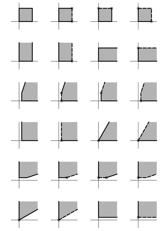
Figure 2. The hemispaces in dimension $2$ which can be obtained as unions of sectors of the same type based at points with full support $\{1,2\}$.

Figure 3. The hemispaces in dimension $2$ which can be obtained as unions of sectors of the same type based at points with non-full support ($\{1\}$ or $\{2\}$).

4. Tropical hemispaces

4.1. Homogenization and $(P,R)$-decompositions.

Let us start with $(P,R)$-decompositions of quasisectors and sectors.

Proposition 4.1.

For $y\in{\mathbb{T}}^{n}$ and $i\in\operatorname{supp}(y)$, the quasisectors ${{\mathcal{W}}}_{i}(y)$ and the sectors ${{\mathcal{S}}}_{i}(y)$ and ${{\mathcal{S}}}_{n+1}(y)$ can be represented as

(12) $$\begin{split}{{\mathcal{W}}}_{i}(y)&=\operatorname{span}\left(\left\{{\rm e}^{i}\oplus y_{j}y_{i}^{-1}{\rm e}^{j}\mid j\in\operatorname{supp}(y)\right\}\right)\;,\\ {{\mathcal{S}}}_{i}(y)&=\left\{y_{i}{\rm e}^{i}\right\}\oplus\operatorname{span}\left(\left\{{\rm e}^{i}\oplus y_{j}y_{i}^{-1}{\rm e}^{j}\mid j\in\operatorname{supp}(y)\right\}\right)\;,\\ {{\mathcal{S}}}_{n+1}(y)&=\operatorname{conv}\left(\left\{{\mathbbold 0}\right\}\cup\left\{y_{j}{\rm e}^{j}\mid j\in\operatorname{supp}(y)\right\}\right)\;.\end{split}$$

Proof.

We claim that if $x\in{{\mathcal{W}}}_{i}(y)$, then

$$x=\bigoplus_{j\in\operatorname{supp}(y)}y_{i}y_{j}^{-1}x_{j}({\rm e}^{i}\oplus y_{j}y_{i}^{-1}{\rm e}^{j})\;.$$

Indeed, we have

$$\left(\bigoplus_{j\in\operatorname{supp}(y)}y_{i}y_{j}^{-1}x_{j}({\rm e}^{i}\oplus y_{j}y_{i}^{-1}{\rm e}^{j})\right)_{i}=\bigoplus_{j\in\operatorname{supp}(y)}y_{i}y_{j}^{-1}x_{j}=x_{i}$$

since $i\in\operatorname{supp}(y)$ and $y_{i}y_{j}^{-1}x_{j}\leq x_{i}$ for all $j\in\operatorname{supp}(y)$ by Definition 3.5. Furthermore for $k\in\operatorname{supp}(y)\setminus\{i\}$ we have

$$\left(\bigoplus_{j\in\operatorname{supp}(y)}y_{i}y_{j}^{-1}x_{j}({\rm e}^{i}\oplus y_{j}y_{i}^{-1}{\rm e}^{j})\right)_{k}=y_{i}y_{k}^{-1}x_{k}y_{k}y_{i}^{-1}=x_{k},$$

and for $k\in[n]\setminus\operatorname{supp}(y)$ we have

$$\left(\bigoplus_{j\in\operatorname{supp}(y)}y_{i}y_{j}^{-1}x_{j}({\rm e}^{i}\oplus y_{j}y_{i}^{-1}{\rm e}^{j})\right)_{k}=\bigoplus_{j\in\operatorname{supp}(y)}y_{i}y_{j}^{-1}x_{j}({\rm e}^{i}\oplus y_{j}y_{i}^{-1}{\rm e}^{j})_{k}={\mathbbold 0}=x_{k}.$$

This proves our claim. Using this property, we conclude that

$${{\mathcal{W}}}_{i}(y)\subseteq\operatorname{span}\left(\left\{{\rm e}^{i}\oplus y_{j}y_{i}^{-1}{\rm e}^{j}\mid j\in\operatorname{supp}(y)\right\}\right)\;.$$

For the converse inclusion, let us show that the vector ${\rm e}^{i}\oplus y_{j}y_{i}^{-1}{\rm e}^{j}$ belongs to ${{\mathcal{W}}}_{i}(y)$ for any $j\in\operatorname{supp}(y)$. Indeed, we have $\left({\rm e}^{i}\oplus y_{j}y_{i}^{-1}{\rm e}^{j}\right)_{k}={\mathbbold 0}$ for any $k\in[n]\setminus\{i,j\}$, and so in particular for any $k\in[n]\setminus\operatorname{supp}(y)$, and

$$\bigoplus_{k\in\operatorname{supp}({\rm e}^{i}\oplus y_{j}y_{i}^{-1}{\rm e}^{j})}\left({\rm e}^{i}\oplus y_{j}y_{i}^{-1}{\rm e}^{j}\right)_{k}y_{k}^{-1}=y_{i}^{-1}\oplus y_{j}y_{i}^{-1}y_{j}^{-1}=y_{i}^{-1}=\left({\rm e}^{i}\oplus y_{j}y_{i}^{-1}{\rm e}^{j}\right)_{i}y_{i}^{-1}\;.$$

Thus, ${\rm e}^{i}\oplus y_{j}y_{i}^{-1}{\rm e}^{j}\in{{\mathcal{W}}}_{i}(y)$ by Definition 3.5. Since ${{\mathcal{W}}}_{i}(y)$ is a cone and ${\rm e}^{i}\oplus y_{j}y_{i}^{-1}{\rm e}^{j}\in{{\mathcal{W}}}_{i}(y)$ for any $j\in\operatorname{supp}(y)$, we conclude that

$$\operatorname{span}\left(\left\{{\rm e}^{i}\oplus y_{j}y_{i}^{-1}{\rm e}^{j}\mid j\in\operatorname{supp}(y)\right\}\right)\subseteq{{\mathcal{W}}}_{i}(y)\;.$$

This completes the proof of the first equality in (12).

From the first equality in (12) it follows that, given $y\in{\mathbb{T}}^{n}$, for all $i\in\operatorname{supp}(y,{\mathbbold 1})=\operatorname{supp}(y)\cup\{n+1\}$ we have ${{\mathcal{W}}}_{i}(y,{\mathbbold 1})=\operatorname{span}(U_{i})$, where

(13) $$U_{i}=\left\{{\rm e}^{i}\oplus(y,{\mathbbold 1})_{j}(y,{\mathbbold 1})_{i}^{-1}{\rm e}^{j}\mid j\in\operatorname{supp}(y)\cup\{n+1\}\right\}\;.$$

Hence by Definition 3.14 and Proposition 2.8, it follows that for all $i\in\operatorname{supp}(y)\cup\{n+1\}$,

(14) $${{\mathcal{S}}}_{i}(y)=C_{{{\mathcal{W}}}_{i}(y,{\mathbbold 1})}^{{\mathbbold 1}}=C_{\operatorname{span}(U_{i})}^{{\mathbbold 1}}=\operatorname{conv}(P_{U_{i}})\oplus\operatorname{span}(R_{U_{i}})\;,$$

where

(15) $$P_{U_{i}}=\left\{y\in{\mathbb{T}}^{n}\mid\exists\mu\neq{\mathbbold 0},(\mu y,\mu)\in U_{i}\right\}\;,$$

and

(16) $$R_{U_{i}}=\left\{z\in{\mathbb{T}}^{n}\mid(z,{\mathbbold 0})\in U_{i}\right\}\;.$$

Let $i\in\operatorname{supp}(y)$ (hence $i\leq n$). Then by (13) we have

$$U_{i}=\left\{{\rm e}^{i}\oplus y_{j}y_{i}^{-1}{\rm e}^{j}\mid j\in\operatorname{supp}(y)\right\}\cup\left\{{\rm e}^{i}\oplus y_{i}^{-1}{\rm e}^{n+1}\right\}\;.$$

Therefore by (15) $z\in P_{U_{i}}$ if and only if there exists $\mu\neq{\mathbbold 0}$ such that $(\mu z,\mu)={\rm e}^{i}\oplus y_{i}^{-1}{\rm e}^{n+1}$ which yields $\mu=y_{i}^{-1}$ and $y_{i}^{-1}z=\mu z={\rm e}^{i}$, whence $z=y_{i}{\rm e}^{i}$. Thus $P_{U_{i}}=\left\{y_{i}{\rm e}^{i}\right\}$. Furthermore, by (16) $z\in R_{U_{i}}$ if and only if $(z,{\mathbbold 0})={\rm e}^{i}\oplus y_{j}y_{i}^{-1}{\rm e}^{j}$ for some $j\in\operatorname{supp}(y)$. Consequently, by (14), we obtain the second equality of (12).

Finally, let $i=n+1.$ Then by (13),

$$U_{n+1}=\left\{{\rm e}^{n+1}\oplus y_{j}{\rm e}^{j}\mid j\in\operatorname{supp}(y)\right\}\cup\left\{{\rm e}^{n+1}\right\},$$

whence $(z,{\mathbbold 0})\notin U_{n+1}$ for all $z\in{\mathbb{T}}^{n},$ and hence by (16), $R_{U_{n+1}}=\emptyset$. Furthermore, for $\mu\neq{\mathbbold 0}$ we have $(\mu z,\mu)\in U_{n+1}$ if and only if either $(\mu z,\mu)={\rm e}^{n+1}\oplus y_{j}{\rm e}^{j}$ for some $j\in\operatorname{supp}(y)$ or $(\mu z,\mu)={\rm e}^{n+1}$. In the first case we obtain $\mu={\mathbbold 1}$ and $z=\mu z=y_{j}{\rm e}^{j}$ for some $j\in\operatorname{supp}(y)$, and in the second case we obtain $\mu={\mathbbold 1}$ and $z=\mu z={\mathbbold 0}$. Thus by (15), $P_{U_{n+1}}=\left\{{\mathbbold 0}\right\}\cup\left\{y_{j}{\rm e}^{j}\mid j\in\operatorname{supp}(y)\right\}$, whence by $R_{U_{n+1}}=\emptyset$ and (14), we obtain the third equality of (12). ∎

We now obtain $(P,R)$-decompositions of hemispaces (respectively, conical hemispaces) by uniting the $(P,R)$-decompositions of sectors (respectively, quasisectors) contained in them.

Theorem 4.2.

For any hemispace ${\mathcal{H}}\subset{\mathbb{T}}^{n}$ (resp. any conical hemispace ${\mathcal{V}}\subset{\mathbb{T}}^{n}$) a $(P,R)$-decomposition can be obtained by uniting the $(P,R)$-decompositions given in (12) of all ${{\mathcal{S}}}_{i}(y)\subseteq{\mathcal{H}}$ (resp. ${{\mathcal{W}}}_{i}(y)\subseteq{\mathcal{V}}$), where $y\in{\mathcal{H}}$ and $i\in\operatorname{supp}(y)\cup\{n+1\}$ (resp. $y\in{\mathcal{V}}$ and $i\in\operatorname{supp}(y)$).

If ${\mathcal{H}}$ is a hemispace, the resulting $(P,R)$-decomposition is given by

(17) $$\begin{split}P&=\begin{cases}\{y_{i}{\rm e}^{i}\mid{{\mathcal{S}}}_{i}(y)\subseteq{\mathcal{H}}\},\ \text{ if there is no $y\in{\mathbb{T}}^{n}$ such that ${{\mathcal{S}}}_{n+1}(y)\subseteq{\mathcal{H}}$}\\ \{{\mathbbold 0}\}\cup\{y_{i}{\rm e}^{i}\mid{{\mathcal{S}}}_{i}(y)\subseteq{\mathcal{H}}\}\cup\{y_{j}{\rm e}^{j}\mid{{\mathcal{S}}}_{n+1}(y)\subseteq{\mathcal{H}},\;j\in\operatorname{supp}(y)\}\text{ otherwise}.\end{cases}\\ R&=\left\{{\rm e}^{i}\oplus y_{j}y_{i}^{-1}{\rm e}^{j}\mid{{\mathcal{S}}}_{i}(y)\subseteq{\mathcal{H}},\;j\in\operatorname{supp}(y)\right\}\;,\end{split}$$

and if ${\mathcal{V}}$ is a conical hemispace, then we have

(18) $$P=\emptyset\;,\ R=\left\{{\rm e}^{i}\oplus y_{j}y_{i}^{-1}{\rm e}^{j}\mid{{\mathcal{W}}}_{i}(y)\subseteq{\mathcal{V}},\;j\in\operatorname{supp}(y)\right\}\;.$$

Proof.

By Theorem 3.25 any hemispace ${\mathcal{H}}$ can be represented as the convex hull of all the sectors contained in ${\mathcal{H}}$. Consider the $(P,R)$-decomposition of sectors given in the last two lines of (12). The pair of sets $(P,R)$ which determines the $(P,R)$-decomposition of the sector ${{\mathcal{S}}}_{i}(y)$, for any $y\in{\mathbb{T}}^{n}$ and $i\in\operatorname{supp}(y)$, satisfy Condition (iii) of Theorem 2.14 due to the fact that $\operatorname{supp}(y_{i}{\rm e}^{i})\subseteq\operatorname{supp}({\rm e}^{i}\oplus y_{j}y_{i}^{-1}{\rm e}^{j})$ for all $j\in\operatorname{supp}(y)$, and the pair of sets deterining the $(P,R)$-decomposition of the sector ${{\mathcal{S}}}_{n+1}(y)$ satisfies this condition trivially (since $R$ is empty). Therefore we can combine all the $(P,R)$-decompositions of the sectors contained in ${\mathcal{H}}$ (in other words, take the unions of all $P$ and all $R$ separately) to obtain a $(P,R)$-decomposition of ${\mathcal{H}}$. To form the set $P$, let us first collect, using Theorem 3.25 and the second line of (12), all the vectors $y_{i}e^{i}$ such that ${{\mathcal{S}}}_{i}(y)\subseteq{\mathcal{H}}$ (where $i\in\operatorname{supp}(y)$). If we have ${{\mathcal{S}}}_{n+1}(y)\subseteq{\mathcal{H}}$ for some $y\in{\mathbb{T}}^{n}$ then, using Theorem 3.25 and the third line of (12), we also add the zero vector and all the vectors $y_{j}{\rm e}^{j}$, where $j\in\operatorname{supp}(y)$. This explains the expression for $P$ in (17), in both cases. The set $R$ is composed of the vectors ${\rm e}^{i}\oplus y_{j}y_{i}^{-1}{\rm e}^{j}$ appearing on the second line of (12), such that ${{\mathcal{S}}}_{i}(y)\subseteq{\mathcal{H}}$ and $j\in\operatorname{supp}(y)$. This explains the last line of (17).

By Theorem 3.12, any conical hemispace ${\mathcal{V}}$ is the linear span of all the quasisectors contained in ${\mathcal{V}}$. Consider the $(P,R)$-decomposition of quasisectors given in the first line of (12). By Lemma 2.15 the union of all the sets $R$ appearing in these $(P,R)$-decompositions of the quasisectors contained in ${\mathcal{V}}$ gives the set $R$ appearing in a $(P,R)$-decomposition of ${\mathcal{V}}$ (in which $P=\emptyset$). By Theorem 3.12 and the first line of (12), $R$ consists of all the vectors ${\rm e}^{i}\oplus y_{j}y_{i}^{-1}{\rm e}^{j}$ such that ${{\mathcal{W}}}_{i}(y)\subseteq{\mathcal{V}}$ and $j\in\operatorname{supp}(y)$. This shows (18). ∎

Let us make an observation on the $(P,R)$-decomposition of Theorem 4.2.

Lemma 4.3.

Let ${\mathcal{H}}\subseteq{\mathbb{T}}^{n}$ be a hemispace, $z\in{\mathbb{T}}^{n}$, and let $R$ be defined by the last line of (17). If ${{\mathcal{S}}}_{i}(z)\subseteq{\mathcal{H}}$ then $z\in\operatorname{span}(R)$.

Proof.

Since ${{\mathcal{S}}}_{i}(z)\subseteq{\mathcal{H}}$, by the last line of (17) the set $R$ contains all the vectors of the form ${\rm e}^{i}\oplus z_{j}z_{i}^{-1}{\rm e}^{j}$ for $j\in\operatorname{supp}(z)$. Representing

$$z=z_{i}\left(\bigoplus_{j\in\operatorname{supp}(z)}({\rm e}^{i}\oplus z_{j}z_{i}^{-1}{\rm e}^{j})\right)\,,$$

we conclude that $z\in\operatorname{span}(R)$. ∎

We shall need the following characterization of joined pairs of conical hemispaces by means of sections.

Lemma 4.4.

Let ${\mathcal{V}}_{1},{\mathcal{V}}_{2}\subseteq{\mathbb{T}}^{n+1}$ be cones. Then, $({\mathcal{V}}_{1},{\mathcal{V}}_{2})$ is a joined pair of conical hemispaces if and only if the following statements hold:

(19) $$C_{{\mathcal{V}}_{1}}^{\alpha}\cap C_{{\mathcal{V}}_{2}}^{\alpha}=\emptyset\;\text{ and }\;C_{{\mathcal{V}}_{1}}^{\alpha}\cup C_{{\mathcal{V}}_{2}}^{\alpha}={\mathbb{T}}^{n}\ \text{for all }\alpha\neq{\mathbbold 0},$$

(20) $$C_{{\mathcal{V}}_{1}}^{{\mathbbold 0}}\cap C_{{\mathcal{V}}_{2}}^{{\mathbbold 0}}=\{{\mathbbold 0}\}\;\text{ and }\;C_{{\mathcal{V}}_{1}}^{{\mathbbold 0}}\cup C_{{\mathcal{V}}_{2}}^{{\mathbbold 0}}={\mathbb{T}}^{n}.$$

Proof.

Assume that $({\mathcal{V}}_{1},{\mathcal{V}}_{2})$ is a joined pair of conical hemispaces, i.e. ${\mathcal{V}}_{1}\cup{\mathcal{V}}_{2}={\mathbb{T}}^{n+1}$ and ${\mathcal{V}}_{1}\cap{\mathcal{V}}_{2}=\{{\mathbbold 0}\}$.

Let $\alpha\in{\mathbb{T}}$. Then, given any $x\in{\mathbb{T}}^{n}$, since ${\mathcal{V}}_{1}\cup{\mathcal{V}}_{2}={\mathbb{T}}^{n+1}$ we have $(x,\alpha)\in{\mathcal{V}}_{1}\cup{\mathcal{V}}_{2}$, and so $x\in C_{{\mathcal{V}}_{1}}^{\alpha}\cup C_{{\mathcal{V}}_{2}}^{\alpha}$. Since $x\in{\mathbb{T}}^{n}$ is arbitrary, this shows $C_{{\mathcal{V}}_{1}}^{\alpha}\cup C_{{\mathcal{V}}_{2}}^{\alpha}={\mathbb{T}}^{n}$ for any $\alpha\in{\mathbb{T}}$.

Suppose now that $\alpha\neq{\mathbbold 0}$ and $C_{{\mathcal{V}}_{1}}^{\alpha}\cap C_{{\mathcal{V}}_{2}}^{\alpha}\neq\emptyset$. Let $x\in C_{{\mathcal{V}}_{1}}^{\alpha}\cap C_{{\mathcal{V}}_{2}}^{\alpha}$. Then, we have $(x,\alpha)\in{\mathcal{V}}_{1}\cap{\mathcal{V}}_{2}$, which contradicts the fact that ${\mathcal{V}}_{1}\cap{\mathcal{V}}_{2}=\{{\mathbbold 0}\}$ because $\alpha\neq{\mathbbold 0}$. This proves that $C_{{\mathcal{V}}_{1}}^{\alpha}\cap C_{{\mathcal{V}}_{2}}^{\alpha}=\emptyset$ for $\alpha\neq{\mathbbold 0}$.

Since ${\mathbbold 0}\in{\mathcal{V}}_{1}\cap{\mathcal{V}}_{2}$, we have ${\mathbbold 0}\in C_{{\mathcal{V}}_{1}}^{{\mathbbold 0}}\cap C_{{\mathcal{V}}_{2}}^{{\mathbbold 0}}$. Furthermore, if for $x\neq{\mathbbold 0}$ we had $x\in C_{{\mathcal{V}}_{1}}^{{\mathbbold 0}}\cap C_{{\mathcal{V}}_{2}}^{{\mathbbold 0}}$, then the non-null vector $(x,{\mathbbold 0})$ would belong to ${\mathcal{V}}_{1}\cap{\mathcal{V}}_{2}$, contradicting the fact that ${\mathcal{V}}_{1}\cap{\mathcal{V}}_{2}=\{{\mathbbold 0}\}$. This shows that $C_{{\mathcal{V}}_{1}}^{{\mathbbold 0}}\cap C_{{\mathcal{V}}_{2}}^{{\mathbbold 0}}=\{{\mathbbold 0}\}$, and completes the proof of (19) and (20).

Assume now that (19) and (20) are satisfied.

Given any $x\in{\mathbb{T}}^{n}$ and $\alpha\in{\mathbb{T}}$, since $C_{{\mathcal{V}}_{1}}^{\alpha}\cup C_{{\mathcal{V}}_{2}}^{\alpha}={\mathbb{T}}^{n}$, we have $x\in C_{{\mathcal{V}}_{1}}^{\alpha}\cup C_{{\mathcal{V}}_{2}}^{\alpha}$. It follows that $(x,\alpha)\in{\mathcal{V}}_{1}\cup{\mathcal{V}}_{2}$. Since $x\in{\mathbb{T}}^{n}$ and $\alpha\in{\mathbb{T}}$ are arbitrary, we conclude that ${\mathcal{V}}_{1}\cup{\mathcal{V}}_{2}={\mathbb{T}}^{n+1}$.

Finally, let $(x,\alpha)\in{\mathcal{V}}_{1}\cap{\mathcal{V}}_{2}$. Then $x\in C_{{\mathcal{V}}_{1}}^{\alpha}\cap C_{{\mathcal{V}}_{2}}^{\alpha}$, and by (19) and (20) we necessarily have $x={\mathbbold 0}$ and $\alpha={\mathbbold 0}$. This shows that ${\mathcal{V}}_{1}\cap{\mathcal{V}}_{2}=\{{\mathbbold 0}\}$, and completes the proof of the fact that $({\mathcal{V}}_{1},{\mathcal{V}}_{2})$ is a joined pair of conical hemispaces. ∎

The following theorem relates complementary pairs of hemispaces in ${\mathbb{T}}^{n}$ with joined pairs of conical hemispaces in ${\mathbb{T}}^{n+1}$ through the concept of section.

Theorem 4.5.

Let ${\mathcal{H}}_{1},{\mathcal{H}}_{2}\subseteq{\mathbb{T}}^{n}$ be a complementary pair of hemispaces, and let $(P_{1},R_{1})$ and $(P_{2},R_{2})$ determine respectively the $(P,R)$-decompositions of ${\mathcal{H}}_{1}$ and ${\mathcal{H}}_{2}$ given by Theorem 4.2. Then, the cones

(21) $${\mathcal{V}}_{1}:=\operatorname{span}\left(\left\{(x,{\mathbbold 1})\mid x\in P_{1}\right\}\cup\left\{(y,{\mathbbold 0})\mid y\in R_{1}\right\}\right)$$

and

(22) $${\mathcal{V}}_{2}:=\operatorname{span}\left(\left\{(x,{\mathbbold 1})\mid x\in P_{2}\right\}\cup\left\{(y,{\mathbbold 0})\mid y\in R_{2}\right\}\right)$$

satisfy ${\mathcal{H}}_{1}=C_{{\mathcal{V}}_{1}}^{{\mathbbold 1}}$ and ${\mathcal{H}}_{2}=C_{{\mathcal{V}}_{2}}^{{\mathbbold 1}}$, and $({\mathcal{V}}_{1},{\mathcal{V}}_{2})$ is a joined pair of conical hemispaces in ${\mathbb{T}}^{n+1}$.

Proof.

In the first place, observe that by Corollary 2.9 we have $C_{{\mathcal{V}}_{1}}^{{\mathbbold 1}}={\mathcal{H}}_{1}$ and $C_{{\mathcal{V}}_{2}}^{{\mathbbold 1}}={\mathcal{H}}_{2}$

To prove that $({\mathcal{V}}_{1},{\mathcal{V}}_{2})$ is a joined pair of conical hemispaces, we show that (19) and (20) are satisfied and then use Lemma 4.4.

Let us first prove (19). Since $({\mathcal{H}}_{1},{\mathcal{H}}_{2})=(C_{{\mathcal{V}}_{1}}^{{\mathbbold 1}},C_{{\mathcal{V}}_{2}}^{{\mathbbold 1}})$ is a complementary pair of hemispaces, it follows that (19) holds for $\alpha={\mathbbold 1}$. For the case of general $\alpha\neq{\mathbbold 0}$, observe that

(23) $$C_{{\mathcal{V}}_{1}\cap{\mathcal{V}}_{2}}^{\alpha}=C_{{\mathcal{V}}_{1}}^{\alpha}\cap C_{{\mathcal{V}}_{2}}^{\alpha}\text{ and }C_{{\mathcal{V}}_{1}\cup{\mathcal{V}}_{2}}^{\alpha}=C_{{\mathcal{V}}_{1}}^{\alpha}\cup C_{{\mathcal{V}}_{2}}^{\alpha}\text{ for all }\alpha\in{\mathbb{T}}\;.$$

Since ${\mathcal{V}}_{1}\cap{\mathcal{V}}_{2}$ and ${\mathcal{V}}_{1}\cup{\mathcal{V}}_{2}$ are closed under multiplication by scalars, using (23) and Proposition 2.7 we conclude that

$$\begin{split}C_{{\mathcal{V}}_{1}}^{\alpha}\cap C_{{\mathcal{V}}_{2}}^{\alpha}&=C_{{\mathcal{V}}_{1}\cap{\mathcal{V}}_{2}}^{\alpha}=\{\alpha x\mid x\in C_{{\mathcal{V}}_{1}\cap{\mathcal{V}}_{2}}^{{\mathbbold 1}}\}=\{\alpha x\mid x\in C_{{\mathcal{V}}_{1}}^{{\mathbbold 1}}\cap C_{{\mathcal{V}}_{2}}^{{\mathbbold 1}}\}=\{\alpha x\mid x\in{\mathcal{H}}_{1}\cap{\mathcal{H}}_{2}\}=\emptyset\;,\\ C_{{\mathcal{V}}_{1}}^{\alpha}\cup C_{{\mathcal{V}}_{2}}^{\alpha}&=C_{{\mathcal{V}}_{1}\cup{\mathcal{V}}_{2}}^{\alpha}=\{\alpha x\mid x\in C_{{\mathcal{V}}_{1}\cup{\mathcal{V}}_{2}}^{{\mathbbold 1}}\}=\{\alpha x\mid x\in C_{{\mathcal{V}}_{1}}^{{\mathbbold 1}}\cup C_{{\mathcal{V}}_{2}}^{{\mathbbold 1}}\}=\{\alpha x\mid x\in{\mathcal{H}}_{1}\cup{\mathcal{H}}_{2}\}={\mathbb{T}}^{n}\;.\end{split}$$

Thus we obtained (19).

It remains to prove (20). Equations (21) and (22) imply that $C_{{\mathcal{V}}_{1}}^{{\mathbbold 0}}=\operatorname{span}(R_{1})$ and $C_{{\mathcal{V}}_{2}}^{{\mathbbold 0}}=\operatorname{span}(R_{2})$, so it remains to show that $(\operatorname{span}(R_{1}),\operatorname{span}(R_{2}))$ is a joined pair of conical hemispaces of ${\mathbb{T}}^{n}$.

Let us show first that $\operatorname{span}(R_{1})\cup\operatorname{span}(R_{2})={\mathbb{T}}^{n}$. Take a vector $z\in{\mathbb{T}}^{n}$. As $({\mathcal{H}}_{1},{\mathcal{H}}_{2})$ is a complementary pair of hemispaces, either $z\in{\mathcal{H}}_{1}$ or $z\in{\mathcal{H}}_{2}$. Assume $z\in{\mathcal{H}}_{1}$. By Theorem 3.20 (taking ${\mathcal{H}}_{2}$ as ${\mathcal{C}}$ and ${\mathcal{H}}_{1}$ as its complement), it follows that ${{\mathcal{S}}}_{i}(z)\subseteq{\mathcal{H}}_{1}$ for $i=n+1$ or for some $i\in\operatorname{supp}(z)$. If ${{\mathcal{S}}}_{i}(z)\subseteq{\mathcal{H}}_{1}$ for some $i\neq n+1$, then $z\in\operatorname{span}(R_{1})$ by Lemma 4.3. In the case when ${{\mathcal{S}}}_{i}(z)\not\subseteq{\mathcal{H}}_{1}$ for any $i\neq n+1$, we have ${{\mathcal{S}}}_{n+1}(z)\subseteq{\mathcal{H}}_{1}$, and we consider $\alpha z$ for $\alpha\neq{\mathbbold 0}$.

Suppose that for some $\alpha\neq{\mathbbold 0}$ we have ${{\mathcal{S}}}_{n+1}(\alpha z)\not\subseteq{\mathcal{H}}_{1}$ and ${{\mathcal{S}}}_{n+1}(\alpha z)\not\subseteq{\mathcal{H}}_{2}$. Then ${{\mathcal{S}}}_{i}(\alpha z)\subseteq{\mathcal{H}}_{1}$ or ${{\mathcal{S}}}_{i}(\alpha z)\subseteq{\mathcal{H}}_{2}$ for some $i\neq n+1$, by Theorem 3.20. If ${{\mathcal{S}}}_{i}(\alpha z)\subseteq{\mathcal{H}}_{1}$ then $z\in\operatorname{span}(R_{1})$, and if ${{\mathcal{S}}}_{i}(\alpha z)\subseteq{\mathcal{H}}_{2}$ then $z\in\operatorname{span}(R_{2})$, by Lemma 4.3, so $z\in\operatorname{span}(R_{1})\cup\operatorname{span}(R_{2})$.

We are left with the case when ${{\mathcal{S}}}_{n+1}(\alpha z)\subseteq{\mathcal{H}}_{1}$ or ${{\mathcal{S}}}_{n+1}(\alpha z)\subseteq{\mathcal{H}}_{2}$ for each $\alpha$. Since by Lemma 3.16 the sets ${{\mathcal{S}}}_{n+1}(\alpha z)$ are increasing with $\alpha$, it can be only that either ${{\mathcal{S}}}_{n+1}(\alpha z)\subseteq{\mathcal{H}}_{1}$ for all $\alpha$, or ${{\mathcal{S}}}_{n+1}(\alpha z)\subseteq{\mathcal{H}}_{2}$ for all $\alpha$. Assume the first case. Then, we obtain that all vectors $x$ with $\operatorname{supp}(x)\subseteq\operatorname{supp}(z)$ are in ${\mathcal{H}}_{1}$, since $x\in{{\mathcal{S}}}_{n+1}(\alpha z)$ with $\alpha=\oplus_{i\in\operatorname{supp}(z)}x_{i}z_{i}^{-1}$ holds for every such $x$. But then ${{\mathcal{S}}}_{i}(z)\subseteq{\mathcal{H}}_{1}$ for any $i\in\operatorname{supp}(z)$, implying that $z\in\operatorname{span}(R_{1})$.

We have shown that if $z\in{\mathcal{H}}_{1}$ then $z\in\operatorname{span}(R_{1})\cup\operatorname{span}(R_{2})$. The same statement holds in the case of $z\in{\mathcal{H}}_{2}$ (by symmetry). Thus $\operatorname{span}(R_{1})\cup\operatorname{span}(R_{2})={\mathbb{T}}^{n}$ is proved, and it remains to show that $\operatorname{span}(R_{1})\cap\operatorname{span}(R_{2})=\{{\mathbbold 0}\}$.

Assume by contradiction that $z\in\operatorname{span}(R_{1})\cap\operatorname{span}(R_{2})$ and $z\neq{\mathbbold 0}$. As $z\in\operatorname{span}(R_{1})$, we have $z=\oplus_{x\in R_{1}}\beta_{x}x$, where only a finite number of the scalars $\beta_{x}$ are not equal to ${\mathbbold 0}$. Observe that $R_{1}\neq\emptyset$ and at least one $\beta_{x}$ is not equal to ${\mathbbold 0}$ because $z\neq{\mathbbold 0}$. By (17), $R_{1}$ is composed of vectors of the form ${\rm e}^{i}\oplus y_{j}y_{i}^{-1}{\rm e}^{j}$, where $y\in{\mathbb{T}}^{n}$ and $i,j\in\operatorname{supp}(y)$ are such that ${{\mathcal{S}}}_{i}(y)\subseteq{\mathcal{H}}_{1}$. Consequently we have $\beta({\rm e}^{i}\oplus y_{j}y_{i}^{-1}{\rm e}^{j})\leq z$ for some $\beta\in{\mathbb{T}}_{+}$, $y\in{\mathbb{T}}^{n}$ and $i,j\in\operatorname{supp}(y)$ such that ${{\mathcal{S}}}_{i}(y)\subseteq{\mathcal{H}}_{1}$. Since ${{\mathcal{S}}}_{i}(y)\subseteq{\mathcal{H}}_{1}$, by (17) it follows that $y_{i}{\rm e}^{i}\in P_{1}$. As $z\in\operatorname{span}(R_{2})$, for the same reasons as above there also exist $\beta^{\prime}\in{\mathbb{T}}_{+}$, $y^{\prime}\in{\mathbb{T}}^{n}$ and $i^{\prime},j^{\prime}\in\operatorname{supp}(y^{\prime})$ such that $\beta^{\prime}({\rm e}^{i^{\prime}}\oplus y^{\prime}_{j^{\prime}}(y^{\prime}_{i^{\prime}})^{-1}{\rm e}^{j^{\prime}})\leq z$ and $y^{\prime}_{i^{\prime}}{\rm e}^{i^{\prime}}\in P_{2}$.

If $\lambda\geq(y_{i}\beta^{-1}\oplus y^{\prime}_{i^{\prime}}(\beta^{\prime})^{-1})$ then $\lambda\geq y_{i}\beta^{-1}$, whence using also that $\beta{\rm e}^{i}\leq z$, we obtain $y_{i}{\rm e}^{i}=y_{i}\beta\beta^{-1}{\rm e}^{i}\leq\lambda\beta{\rm e}^{i}\leq\lambda z.$ Similarly, since $\lambda\geq y^{\prime}_{i^{\prime}}(\beta^{\prime})^{-1},$ we obtain $y^{\prime}_{i^{\prime}}{\rm e}^{i^{\prime}}\leq\lambda z$. These inequalities can be written as equalities $y_{i}{\rm e}^{i}\oplus\lambda z=y^{\prime}_{i^{\prime}}{\rm e}^{i^{\prime}}\oplus\lambda z=\lambda z$, whence $\lambda z\in\operatorname{conv}(P_{1})\oplus\operatorname{span}(R_{1})={\mathcal{H}}_{1}$ and $\lambda z\in\operatorname{conv}(P_{2})\oplus\operatorname{span}(R_{2})={\mathcal{H}}_{2}$, so $\lambda z\in{\mathcal{H}}_{1}\cap{\mathcal{H}}_{2}$, in contradiction with the assumption ${\mathcal{H}}_{1}\cap{\mathcal{H}}_{2}=\emptyset$. Thus the proof of (19) and (20) is complete and Lemma 4.4 implies that $({\mathcal{V}}_{1},{\mathcal{V}}_{2})$ is a joined pair of conical hemispaces. ∎

4.2. On the $(P,R)$-decomposition of conical hemispaces

We know that the $(P,R)$-decomposition of a conical hemispace, as a linear span of quasisectors (Theorem 3.12), consists of unit vectors and linear combinations of two unit vectors (Theorem 4.2). Therefore, to describe the $(P,R)$-decompositions of a joined pair of conical hemispaces we need to understand how the linear combinations of two unit vectors are distributed among them. With this aim, we first associate with a non-trivial joined pair $({\mathcal{V}}_{1},{\mathcal{V}}_{2})$ of conical hemispaces in ${\mathbb{T}}^{n}$ the index sets

(24) $$I:=\left\{i\in[n]\mid{\rm e}^{i}\in{\mathcal{V}}_{1}\right\}\;\makebox{ and }\;J:=\left\{j\in[n]\mid{\rm e}^{j}\in{\mathcal{V}}_{2}\right\}.$$

The following lemma is elementary and will rather serve to define below the coefficients $\alpha_{ij}$. In what follows, for some purposes it will be convenient to assume that scalars can also take the value $+\infty$ (the structure which is obtained defining $\lambda\oplus(+\infty):=+\infty,(+\infty)\oplus\lambda:=+\infty$ for $\lambda\in{\mathbb{T}}$, $\lambda\otimes(+\infty):=+\infty,(+\infty)\otimes\lambda:=+\infty$ for $\lambda\in{\mathbb{T}}_{+}$ and ${\mathbbold 0}\otimes(+\infty):={\mathbbold 0},(+\infty)\otimes{\mathbbold 0}:={\mathbbold 0}$ is usually known as the completed semifield, see for instance [9]) and to adopt the convention

(25) $${\rm e}^{i}\oplus\lambda{\rm e}^{j}={\rm e}^{j}\text{ if }\lambda=+\infty\;.$$

Lemma 4.6.

Let $({\mathcal{V}}_{1},{\mathcal{V}}_{2})$ be a non-trivial joined pair of conical hemispaces of ${\mathbb{T}}^{n}$, and let $I,J\subset[n]$ be defined as in (24). Then, for any $i\in I$ and $j\in J$ we have

$$\sup\left\{\alpha\in{\mathbb{T}}\cup\{+\infty\}\mid{\rm e}^{i}\oplus\alpha{\rm e}^{j}\in{\mathcal{V}}_{1}\right\}=\inf\left\{\beta\in{\mathbb{T}}\cup\{+\infty\}\mid{\rm e}^{i}\oplus\beta{\rm e}^{j}\in{\mathcal{V}}_{2}\right\}.$$

Proof.

In the sequel, we will use the fact that every linear combination of two unit vectors belongs either to ${\mathcal{V}}_{1}$ or to ${\mathcal{V}}_{2}$, which follows from ${\mathcal{V}}_{1}\cap{\mathcal{V}}_{2}=\{{\mathbbold 0}\}$ and ${\mathcal{V}}_{1}\cup{\mathcal{V}}_{2}={\mathbb{T}}^{n}$.

First, assume that $\inf\left\{\beta\in{\mathbb{T}}\cup\{+\infty\}\mid{\rm e}^{i}\oplus\beta{\rm e}^{j}\in{\mathcal{V}}_{2}\right\}=+\infty$, which implies ${\rm e}^{i}\oplus\beta{\rm e}^{j}\not\in{\mathcal{V}}_{2}$ for all $\beta\in{\mathbb{T}}$. Then, we have ${\rm e}^{i}\oplus\alpha{\rm e}^{j}\in{\mathcal{V}}_{1}$ for all $\alpha\in{\mathbb{T}}$, and so $\sup\left\{\alpha\in{\mathbb{T}}\cup\{+\infty\}\mid{\rm e}^{i}\oplus\alpha{\rm e}^{j}\in{\mathcal{V}}_{1}\right\}=+\infty$.

Assume now that $\inf\left\{\beta\in{\mathbb{T}}\cup\{+\infty\}\mid{\rm e}^{i}\oplus\beta{\rm e}^{j}\in{\mathcal{V}}_{2}\right\}\neq+\infty$. Observe that we have the following implication:

(26) $${\rm e}^{i}\oplus\beta{\rm e}^{j}\in{\mathcal{V}}_{2}\;,\;\gamma\geq\beta\Rightarrow{\rm e}^{i}\oplus\gamma{\rm e}^{j}\in{\mathcal{V}}_{2}\;,$$

since ${\rm e}^{j}\in{\mathcal{V}}_{2}$ and, further, ${\rm e}^{i}\oplus\gamma{\rm e}^{j}=({\rm e}^{i}\oplus\beta{\rm e}^{j})\oplus\gamma{\rm e}^{j}\in{\mathcal{V}}_{2}$ if $\gamma\geq\beta$. Thus,

(27) $$\sup\left\{\alpha\in{\mathbb{T}}\cup\{+\infty\}\mid{\rm e}^{i}\oplus\alpha{\rm e}^{j}\in{\mathcal{V}}_{1}\right\}\leq\inf\left\{\beta\in{\mathbb{T}}\cup\{+\infty\}\mid{\rm e}^{i}\oplus\beta{\rm e}^{j}\in{\mathcal{V}}_{2}\right\}\;,$$

because if we had $>$ in (27), then there would exist $\alpha,\beta\in{\mathbb{T}}$ with $\alpha>\beta$ such that ${\rm e}^{i}\oplus\alpha{\rm e}^{j}\in{\mathcal{V}}_{1}$ and ${\rm e}^{i}\oplus\beta{\rm e}^{j}\in{\mathcal{V}}_{2}$. Then by ${\rm e}^{i}\oplus\beta{\rm e}^{j}\in{\mathcal{V}}_{2}$ and (26) it would follow that ${\rm e}^{i}\oplus\alpha{\rm e}^{j}\in{\mathcal{V}}_{2}$, whence ${\rm e}^{i}\oplus\alpha{\rm e}^{j}\notin{\mathcal{V}}_{1}$, a contradiction. If $\inf\left\{\beta\in{\mathbb{T}}\cup\{+\infty\}\mid{\rm e}^{i}\oplus\beta{\rm e}^{j}\in{\mathcal{V}}_{2}\right\}={\mathbbold 0}$, then the lemma follows from (27). Thus, it remains to consider the case $\inf\left\{\beta\in{\mathbb{T}}\cup\{+\infty\}\mid{\rm e}^{i}\oplus\beta{\rm e}^{j}\in{\mathcal{V}}_{2}\right\}\in{\mathbb{T}}_{+}$. In this case, by the definition of $\inf$ we have ${\rm e}^{i}\oplus\alpha{\rm e}^{j}\not\in{\mathcal{V}}_{2}$ for all $\alpha<\inf\left\{\beta\in{\mathbb{T}}\cup\{+\infty\}\mid{\rm e}^{i}\oplus\beta{\rm e}^{j}\in{\mathcal{V}}_{2}\right\}$. Then, since every linear combination of two unit vectors belongs either to ${\mathcal{V}}_{1}$ or to ${\mathcal{V}}_{2}$, we have ${\rm e}^{i}\oplus\alpha{\rm e}^{j}\in{\mathcal{V}}_{1}$ for all $\alpha<\inf\left\{\beta\in{\mathbb{T}}\cup\{+\infty\}\mid{\rm e}^{i}\oplus\beta{\rm e}^{j}\in{\mathcal{V}}_{2}\right\}$, and so (27) must be satisfied with equality. This completes the proof. ∎

Henceforth, the matrix whose entries are the coefficients

(28) $$\alpha_{ij}:=\sup\left\{\alpha\in{\mathbb{T}}\cup\{+\infty\}\mid{\rm e}^{i}\oplus\alpha{\rm e}^{j}\in{\mathcal{V}}_{1}\right\}=\inf\left\{\beta\in{\mathbb{T}}\cup\{+\infty\}\mid{\rm e}^{i}\oplus\beta{\rm e}^{j}\in{\mathcal{V}}_{2}\right\}$$

will be referred to as the $\alpha$-matrix (associated with the non-trivial joined pair $({\mathcal{V}}_{1},{\mathcal{V}}_{2})$ of conical hemispaces). Besides, with each coefficient $\alpha_{ij}$ we associate the pair of subsets of ${\mathbb{T}}\cup\{+\infty\}$ defined by

(29) $$(\alpha_{ij}^{(-)},\alpha_{ij}^{(+)}):=\begin{cases}(\{\lambda\mid\lambda<\alpha_{ij}\},\{\lambda\mid\lambda\geq\alpha_{ij}\})&\text{ if }\alpha_{ij}\in{\mathbb{T}}_{+},{\rm e}^{i}\oplus\alpha_{ij}{\rm e}^{j}\in{\mathcal{V}}_{2},\\ (\{\lambda\mid\lambda\leq\alpha_{ij}\},\{\lambda\mid\lambda>\alpha_{ij}\})&\text{ if }\alpha_{ij}\in{\mathbb{T}}_{+},{\rm e}^{i}\oplus\alpha_{ij}{\rm e}^{j}\in{\mathcal{V}}_{1},\\ (\{\alpha_{ij}\},\{\lambda\mid\lambda>\alpha_{ij}\})&\text{ if }\alpha_{ij}={\mathbbold 0},\\ (\{\lambda\mid\lambda<\alpha_{ij}\},\{\alpha_{ij}\})&\text{ if }\alpha_{ij}=+\infty.\end{cases}$$

Thus, by Lemma 4.6 it follows that

(30) $$\left\{{\rm e}^{i}\oplus\lambda{\rm e}^{j}\mid\lambda\in\alpha_{ij}^{(-)}\right\}\subset{\mathcal{V}}_{1}\makebox{ and }\left\{{\rm e}^{i}\oplus\lambda{\rm e}^{j}\mid\lambda\in\alpha_{ij}^{(+)}\right\}\subset{\mathcal{V}}_{2}$$

for any $i\in I$ and $j\in J$.

Since $\alpha_{ij}^{(+)}\subseteq{\mathbb{T}}_{+}\cup\{+\infty\}$ and $\alpha_{ij}^{(-)}\subseteq{\mathbb{T}}_{+}\cup\{{\mathbbold 0}\}$, observe that the sets $\alpha_{i_{1}j_{1}}^{(+)}$ and $\alpha_{i_{2}j_{2}}^{(+)}$, as well as $\alpha_{i_{1}j_{1}}^{(-)}$ and $\alpha_{i_{2}j_{2}}^{(-)}$, can be unambiguously multiplied (by definition, the product of two sets consists of all possible products of an element of one set by an element of the other set) for any $i_{1},i_{2}\in I$ and $j_{1},j_{2}\in J$.

In the sequel, we write $I^{1}+\cdots+I^{m}=I$ if $I^{k}$ for $k\in[m]$ and $I$ are index sets such that $I^{1}\cup\cdots\cup I^{m}=I$ and $I^{1},\ldots,I^{m}$ are pairwise disjoint.

We now formulate one of the main results of the paper: a characterization of conical hemispaces in terms of their generators. We will immediately prove that any conical hemispaces fulfils the given conditions. The proof that these conditions are also sufficient is going to occupy the remaining part of this section.

Theorem 4.7.

A non-trivial cone ${\mathcal{V}}\subset{\mathbb{T}}^{n}$ is a conical hemispace if and only if

(31) $${\mathcal{V}}=\operatorname{span}\left(\left\{{\rm e}^{i}\oplus\lambda{\rm e}^{j}\mid i\in I,j\in J,\lambda\in\sigma_{ij}^{(-)}\right\}\right),$$

where $I$ is a non-empty proper subset of $[n]$, $J=[n]\setminus I$, and the sets $\sigma_{ij}^{(-)}$, which are non-empty proper subsets of ${\mathbb{T}}\cup\{+\infty\}$ either of the form $\{\lambda\in{\mathbb{T}}\mid\lambda\leq\sigma_{ij}\}$ or $\{\lambda\in{\mathbb{T}}\mid\lambda<\sigma_{ij}\}$ with $\sigma_{ij}\in{\mathbb{T}}\cup\{+\infty\}$, are such that the pairs $(\sigma^{(-)}_{ij},\sigma^{(+)}_{ij})$, with $\sigma^{(+)}_{ij}$ defined by $\sigma^{(+)}_{ij}:=({\mathbb{T}}\cup\{+\infty\})\setminus\sigma^{(-)}_{ij}$, satisfy

(32) $$\sigma_{i_{1}j_{2}}^{(+)}\sigma_{i_{2}j_{1}}^{(+)}\cap\sigma_{i_{1}j_{1}}^{(-)}\sigma_{i_{2}j_{2}}^{(-)}=\emptyset\;\makebox{ and }\;\sigma_{i_{1}j_{2}}^{(-)}\sigma_{i_{2}j_{1}}^{(-)}\cap\sigma_{i_{1}j_{1}}^{(+)}\sigma_{i_{2}j_{2}}^{(+)}=\emptyset$$

for any $i_{1},i_{2}\in I$ and $j_{1},j_{2}\in J$.

Proof of the “only if” part of Theorem 4.7. Define ${\mathcal{V}}_{1}:={\mathcal{V}}$ and ${\mathcal{V}}_{2}:=\complement{\mathcal{V}}\cup\{{\mathbbold 0}\}$. Thus, $({\mathcal{V}}_{1},{\mathcal{V}}_{2})$ is a non-trivial joined pair of conical hemispaces in ${\mathbb{T}}^{n}$ because ${\mathcal{V}}$ is a conical hemispace and non-trivial. Let $I$ and $J$ be the sets defined in (24). Then, $I$ and $J$ satisfy $J=[n]\setminus I$, and these sets are non-empty since $({\mathcal{V}}_{1},{\mathcal{V}}_{2})$ is non-trivial. For $i\in I$ and $j\in J$, let $\sigma_{ij}:=\alpha_{ij}$ and $(\sigma_{ij}^{(-)},\sigma_{ij}^{(+)}):=(\alpha_{ij}^{(-)},\alpha_{ij}^{(+)})$, where the scalars $\alpha_{ij}$ and the pairs of sets $(\alpha_{ij}^{(-)},\alpha_{ij}^{(+)})$ are defined by (28) and (29) respectively. Then, the sets $\sigma_{ij}^{(-)}$ and $\sigma_{ij}^{(+)}$ are of the required form.

We claim that

(33) $$\begin{split}{\mathcal{V}}_{1}=\operatorname{span}\left(\left\{{\rm e}^{i}\oplus\lambda{\rm e}^{j}\mid i\in I,j\in J,\lambda\in\sigma_{ij}^{(-)}\right\}\right),\\ {\mathcal{V}}_{2}=\operatorname{span}\left(\left\{{\rm e}^{i}\oplus\lambda{\rm e}^{j}\mid i\in I,j\in J,\lambda\in\sigma_{ij}^{(+)}\right\}\right).\end{split}$$

Indeed, by Theorem 4.2 both ${\mathcal{V}}_{1}$ and ${\mathcal{V}}_{2}$ are generated by unit vectors and linear combinations of two unit vectors. The distribution of unit vectors is given by $I$ and $J$. Observe that (33) conforms to this distribution, since for any $i\in I$, ${\rm e}^{i}$ belongs to the generators of ${\mathcal{V}}_{1}$ as ${\mathbbold 0}\in\sigma_{ij}^{(-)}$, and for any $j\in J$, ${\rm e}^{j}$ belongs to the generators of ${\mathcal{V}}_{2}$ since $+\infty\in\sigma_{ij}^{(+)}$. This obviously implies that no linear combination of ${\rm e}^{i_{1}}$ and ${\rm e}^{i_{2}}$ with $i_{1},i_{2}\in I$ (resp. of ${\rm e}^{j_{1}}$ and ${\rm e}^{j_{2}}$ with $j_{1},j_{2}\in J$) is necessary in (33) to generate ${\mathcal{V}}_{1}$ (resp. ${\mathcal{V}}_{2}$). For $i\in I$ and $j\in J$, the distribution of the linear combinations of ${\rm e}^{i}$ and ${\rm e}^{j}$ is given by (30). Since $(\sigma_{ij}^{(-)},\sigma_{ij}^{(+)})=(\alpha_{ij}^{(-)}\alpha_{ij}^{(+)})$, it follows that (33) also conforms to this distribution. These observations yield (33).

It remains to prove (32). Assume that

$$\sigma_{i_{1}j_{2}}^{(+)}\sigma_{i_{2}j_{1}}^{(+)}\cap\sigma_{i_{1}j_{1}}^{(-)}\sigma_{i_{2}j_{2}}^{(-)}\neq\emptyset\;.$$

Then, there exist $\beta_{i_{1}j_{2}}\in\sigma_{i_{1}j_{2}}^{(+)}$, $\beta_{i_{2}j_{1}}\in\sigma_{i_{2}j_{1}}^{(+)}$, $\gamma_{i_{1}j_{1}}\in\sigma_{i_{1}j_{1}}^{(-)}$ and $\gamma_{i_{2}j_{2}}\in\sigma_{i_{2}j_{2}}^{(-)}$ such that $\beta_{i_{1}j_{2}}\beta_{i_{2}j_{1}}=\gamma_{i_{1}j_{1}}\gamma_{i_{2}j_{2}}$. For this to hold, the products $\beta_{i_{1}j_{2}}\beta_{i_{2}j_{1}}$ and $\gamma_{i_{1}j_{1}}\gamma_{i_{2}j_{2}}$ should be in ${\mathbb{T}}_{+}$, and hence $\beta_{i_{1}j_{2}}$, $\beta_{i_{2}j_{1}}$, $\gamma_{i_{1}j_{1}}$ and $\gamma_{i_{2}j_{2}}$ should be in ${\mathbb{T}}_{+}$. Then, we make the linear combination

$$z={\rm e}^{i_{1}}\oplus\beta_{i_{1}j_{2}}{\rm e}^{j_{2}}\oplus\lambda({\rm e}^{i_{2}}\oplus\beta_{i_{2}j_{1}}{\rm e}^{j_{1}})\in{\mathcal{V}}_{2}\;,$$

where $\lambda$ satisfies $\lambda\beta_{i_{2}j_{1}}=\gamma_{i_{1}j_{1}}$, hence also $\lambda\gamma_{i_{2}j_{2}}=\beta_{i_{1}j_{2}}$, and observe that

$$z={\rm e}^{i_{1}}\oplus\gamma_{i_{1}j_{1}}{\rm e}^{j_{1}}\oplus\lambda({\rm e}^{i_{2}}\oplus\gamma_{i_{2}j_{2}}{\rm e}^{j_{2}})\in{\mathcal{V}}_{1}\;.$$

Thus ${\mathcal{V}}_{1}\cap{\mathcal{V}}_{2}\neq\{{\mathbbold 0}\}$, a contradiction. This completes the proof of the “only if” part of Theorem 4.7. The “if” part will be proved later (formally after Remark 4.17, but the preparations for this proof will start right after Corollary 4.9).

The following result shows that if a non-trivial cone ${\mathcal{V}}$ defined as in (31) is a conical hemispace, then $\complement{\mathcal{V}}\cup\{{\mathbbold 0}\}$ can be defined as ${\mathcal{V}}_{2}$ in (33) and the scalars $\sigma_{ij}$ are precisely the entries of the $\alpha$-matrix associated with the non-trivial joined pair of conical hemispaces $({\mathcal{V}},\complement{\mathcal{V}}\cup\{{\mathbbold 0}\})$.

Proposition 4.8.

Assume that

(34) $${\mathcal{V}}_{1}=\operatorname{span}\left(\left\{{\rm e}^{i}\oplus\lambda{\rm e}^{j}\mid i\in I,j\in J,\lambda\in\sigma_{ij}^{(-)}\right\}\right)$$

is a conical hemispace, where $I$ is a non-empty proper subset of $[n]$, $J=[n]\setminus I$, and for $i\in I$ and $j\in J$ the sets $\sigma_{ij}^{(-)}$ are non-empty proper subsets of ${\mathbb{T}}\cup\{+\infty\}$ either of the form $\{\lambda\in{\mathbb{T}}\mid\lambda\leq\sigma_{ij}\}$ or $\{\lambda\in{\mathbb{T}}\mid\lambda<\sigma_{ij}\}$ with $\sigma_{ij}\in{\mathbb{T}}\cup\{+\infty\}$. Then, ${\mathcal{V}}_{1}$ and ${\mathcal{V}}_{2}$ defined by

(35) $${\mathcal{V}}_{2}:=\operatorname{span}\left(\left\{{\rm e}^{i}\oplus\lambda{\rm e}^{j}\mid i\in I,j\in J,\lambda\in\sigma_{ij}^{(+)}\right\}\right),$$

where $\sigma^{(+)}_{ij}:=({\mathbb{T}}\cup\{+\infty\})\setminus\sigma^{(-)}_{ij}$, form a joined pair of conical hemispaces, and we have $\sigma_{ij}=\alpha_{ij}$ for all $i\in I$ and $j\in J$ with $\alpha_{ij}$ defined by (28).

Proof.

Let $R:=\left\{{\rm e}^{i}\oplus\lambda{\rm e}^{j}\mid i\in I,j\in J,\lambda\in\sigma_{ij}^{(-)}\right\}$. We first claim that the unit vectors and linear combinations of two unit vectors contained in ${\mathcal{V}}_{1}$ are precisely the ones in $R$. Indeed given $j\in J$, since ${\rm e}^{j}\not\in R$, it readily follows that ${\rm e}^{j}\not\in{\mathcal{V}}_{1}$. Then, the unit vectors contained in ${\mathcal{V}}_{1}$ are precisely the ones in $R$ (i.e. ${\rm e}^{i}$ for $i\in I$). Assume now that ${\rm e}^{i}\oplus\beta{\rm e}^{j}\in{\mathcal{V}}_{1}$ for some $i\in I$, $j\in J$ and $\beta\in{\mathbb{T}}_{+}$. Then, we have ${\rm e}^{i}\oplus\beta{\rm e}^{j}=\oplus_{y\in R}\delta_{y}y$, where only a finite number of the scalars $\delta_{y}$ is not equal to ${\mathbbold 0}$. Observe that

(36) $$\begin{split}\delta_{y}\neq{\mathbbold 0}&\implies y_{k}={\mathbbold 0}\text{ for }k\in[n]\setminus\{i,j\}\implies y={\rm e}^{i}\oplus\lambda{\rm e}^{j}\text{ for some }\lambda\in\sigma_{ij}^{(-)}\\ &\implies y_{i}={\mathbbold 0},y_{j}\in\sigma_{ij}^{(-)},\text{ and }y_{k}={\mathbbold 0}\text{ for }k\in[n]\setminus\{i,j\}\;.\end{split}$$

Then ${\mathbbold 1}=({\rm e}^{i}\oplus\beta{\rm e}^{j})_{i}=(\oplus_{y\in R}\delta_{y}y)_{i}=\oplus_{y\in R}\delta_{y}y_{i}=\oplus_{y\in R}\delta_{y}$, and so $\delta_{y}\leq{\mathbbold 1}$ for all $y\in R$. Besides, since only a finite number of the scalars $\delta_{y}$ is not equal to ${\mathbbold 0}$ and $\beta=({\rm e}^{i}\oplus\beta{\rm e}^{j})_{j}=(\oplus_{y\in R}\delta_{y}y)_{j}=\oplus_{y\in R}\delta_{y}y_{j}$, we conclude that $\beta=\delta_{y}y_{j}$ for some $y\in R$ such that $\delta_{y}\neq{\mathbbold 0}$. Using (36) and the fact that $\lambda\in\sigma_{ij}^{(-)}$ and $\delta\leq{\mathbbold 1}$ imply $\delta\lambda\in\sigma_{ij}^{(-)}$, it follows that $\beta\in\sigma_{ij}^{(-)}$, and so ${\rm e}^{i}\oplus\beta{\rm e}^{j}\in R$. This completes the proof of our claim.

By Theorem 4.2, the conical hemispace $\complement{\mathcal{V}}_{1}\cup\{{\mathbbold 0}\}$ is generated by the unit vectors and linear combinations of two unit vectors which it contains, i.e. those which do not belong to ${\mathcal{V}}_{1}$. By the first part of the proof and the definition of $\sigma^{(+)}_{ij}$ as complements of $\sigma^{(-)}_{ij}$ in ${\mathbb{T}}\cup\{+\infty\}$, we know that these vectors are precisely the generators of ${\mathcal{V}}_{2}$ in (35). Then ${\mathcal{V}}_{2}=\complement{\mathcal{V}}_{1}\cup\{{\mathbbold 0}\}$, and so ${\mathcal{V}}_{1}$ and ${\mathcal{V}}_{2}$ form a joined pair of conical hemispaces.

Finally, the fact that the entries $\alpha_{ij}$ of the $\alpha$-matrix associated with $({\mathcal{V}}_{1},{\mathcal{V}}_{2})$ coincide with the scalars $\sigma_{ij}$ follows from their definition (28) and from (34) and (35). ∎

Condition (32) will be called the rank-one condition, due to the following observation.

Corollary 4.9.

If condition (32) is satisfied and $\sigma_{ij}\in{\mathbb{T}}_{+}$ for $i\in\{i_{1},i_{2}\}$ and $j\in\{j_{1},j_{2}\}$, then $\sigma_{i_{1}j_{1}}\sigma_{i_{2}j_{2}}=\sigma_{i_{1}j_{2}}\sigma_{i_{2}j_{1}}$. In particular, if all the entries of an $\alpha$-matrix belong to ${\mathbb{T}}_{+}$, then it has rank one.

In the rest of this subsection, we assume that $I$ is a non-empty proper subset of $[n]$ and ${\mathcal{V}}$ is the non-trivial cone defined by (31), where $J:=[n]\setminus I$ and the sets $\sigma_{ij}^{(-)}$, which are either of the form $\{\lambda\in{\mathbb{T}}\mid\lambda\leq\sigma_{ij}\}$ or $\{\lambda\in{\mathbb{T}}\mid\lambda<\sigma_{ij}\}$ with $\sigma_{ij}\in{\mathbb{T}}\cup\{+\infty\}$, are such that the pairs $(\sigma^{(-)}_{ij},\sigma^{(+)}_{ij})$, with $\sigma^{(+)}_{ij}$ defined by $\sigma^{(+)}_{ij}:=({\mathbb{T}}\cup\{+\infty\})\setminus\sigma^{(-)}_{ij}$, satisfy the rank-one condition (32). With the objective of showing that any such cone is a conical hemispace, we first give a detailed description of the “thin structure” of the corresponding $\sigma$-matrix that follows from the rank-one condition (32). This description can be also seen as one of the main results.

Proposition 4.10.

If we define

$$\begin{split}J_{i}^{<}:=&\{j\in J\mid\sigma_{ij}\in{\mathbb{T}}_{+}\;\makebox{and}\;\sigma_{ij}\in\sigma_{ij}^{(+)}\},\\ J_{i}^{\leq}:=&\{j\in J\mid\sigma_{ij}\in{\mathbb{T}}_{+}\;\makebox{and}\;\sigma_{ij}\in\sigma_{ij}^{(-)}\},\\ J_{i}^{{\mathbbold 0}}:=&\{j\in J\mid\sigma_{ij}={\mathbbold 0}\},\\ J_{i}^{\infty}:=&\{j\in J\mid\sigma_{ij}=+\infty\},\end{split}$$

for $i\in I$, then by the rank-one condition (32) it follows that:

1. $J_{i}^{\leq}+J_{i}^{<}+J_{i}^{\infty}+J_{i}^{{\mathbbold 0}}=J$ for each $i\in I$;

2. $J_{i_{1}}^{\infty}\subseteq J_{i_{2}}^{\infty}$ or $J_{i_{2}}^{\infty}\subseteq J_{i_{1}}^{\infty}$, and $J_{i_{1}}^{{\mathbbold 0}}\subseteq J_{i_{2}}^{{\mathbbold 0}}$ or $J_{i_{2}}^{{\mathbbold 0}}\subseteq J_{i_{1}}^{{\mathbbold 0}}$ for any $i_{1},i_{2}\in I$;

3. If $(J_{i_{1}}^{<}\cup J_{i_{1}}^{\leq})\cap(J_{i_{2}}^{<}\cup J_{i_{2}}^{\leq})\neq\emptyset$, then $J_{i_{1}}^{<}\cup J_{i_{1}}^{\leq}=J_{i_{2}}^{<}\cup J_{i_{2}}^{\leq}$, $J_{i_{1}}^{\infty}=J_{i_{2}}^{\infty}$ and $J_{i_{1}}^{{\mathbbold 0}}=J_{i_{2}}^{{\mathbbold 0}}$;

4. If $(J_{i_{1}}^{<}\cup J_{i_{1}}^{\leq})\cap(J_{i_{2}}^{<}\cup J_{i_{2}}^{\leq})\neq\emptyset$, then $J_{i_{1}}^{<}\subseteq J_{i_{2}}^{<}$ or $J_{i_{2}}^{<}\subseteq J_{i_{1}}^{<}$;

5. If $(J_{i_{1}}^{<}\cup J_{i_{1}}^{\leq})\cap(J_{i_{2}}^{<}\cup J_{i_{2}}^{\leq})\neq\emptyset$, then there exists $\lambda\in{\mathbb{T}}_{+}$ such that $\sigma_{i_{1}j}=\lambda\sigma_{i_{2}j}$ for all $j\in J_{i_{1}}^{<}\cup J_{i_{1}}^{\leq}=J_{i_{2}}^{<}\cup J_{i_{2}}^{\leq}$.

Proof.

In this proof, we will use $F$, $\geq F$ and $\leq F$ to represent an entry of a matrix which belongs to ${\mathbb{T}}_{+}$, ${\mathbb{T}}_{+}\cup\{+\infty\}$ and ${\mathbb{T}}_{+}\cup\{{\mathbbold 0}\}={\mathbb{T}}$, respectively.

(i) This property readily follows from the definition of the sets $J_{i}^{<}$, $J_{i}^{\leq}$, $J_{i}^{{\mathbbold 0}}$, and $J_{i}^{\infty}$.

(ii) If these conditions are violated, then the $\sigma$-matrix has one of the following $2\times 2$ minors

$$\begin{pmatrix}+\infty&\leq F\\ \leq F&+\infty\end{pmatrix}\;,\quad\begin{pmatrix}{\mathbbold 0}&\geq F\\ \geq F&{\mathbbold 0}\end{pmatrix}\;,$$

violating (32).

(iii) If this condition is violated, then the $\sigma$-matrix has one of the following $2\times 2$ minors

$$\begin{pmatrix}F&F\\ {\mathbbold 0}&F\end{pmatrix},\quad\begin{pmatrix}F&F\\ +\infty&F\end{pmatrix},\quad\begin{pmatrix}+\infty&F\\ {\mathbbold 0}&F\end{pmatrix},$$

violating (32). More precisely, one of the first two minors will appear when $(J_{i_{1}}^{<}\cup J_{i_{1}}^{\leq})\cap(J_{i_{2}}^{<}\cup J_{i_{2}}^{\leq})\neq\emptyset$ but $(J_{i_{1}}^{<}\cup J_{i_{1}}^{\leq})\neq(J_{i_{2}}^{<}\cup J_{i_{2}}^{\leq})$. The third one will appear if $(J_{i_{1}}^{<}\cup J_{i_{1}}^{\leq})=(J_{i_{2}}^{<}\cup J_{i_{2}}^{\leq})\neq\emptyset$ but $J_{i_{1}}^{\infty}\neq J_{i_{2}}^{\infty}$ (equivalently, $J_{i_{1}}^{{\mathbbold 0}}\neq J_{i_{2}}^{{\mathbbold 0}}$).

(iv) If $J_{i_{1}}^{<}\subseteq J_{i_{2}}^{<}$ and $J_{i_{2}}^{<}\subseteq J_{i_{1}}^{<}$ do not hold for some $i_{1},i_{2}$, then there exist $j_{1}$ and $j_{2}$ such that $\sigma_{i_{1}j_{1}}\in\sigma_{i_{1}j_{1}}^{(+)}$, $\sigma_{i_{2}j_{2}}\in\sigma_{i_{2}j_{2}}^{(+)}$, $\sigma_{i_{1}j_{2}}\in\sigma_{i_{1}j_{2}}^{(-)}$, $\sigma_{i_{2}j_{1}}\in\sigma_{i_{2}j_{1}}^{(-)}$, and $\sigma_{i_{1}j_{1}},\sigma_{i_{1}j_{2}},\sigma_{i_{2}j_{1}},\sigma_{i_{2},j_{2}}\in{\mathbb{T}}_{+}$. However, this contradicts the rank-one condition (32), since $\sigma_{i_{1}j_{1}}\sigma_{i_{2}j_{2}}=\sigma_{i_{1}j_{2}}\sigma_{i_{2}j_{1}}$ by Corollary 4.9.

(v) This property follows from Corollary 4.9 and Property (iii). ∎

Remark 4.11.

Regarding Property (ii) of Proposition 4.10, observe that the condition “$J_{i_{1}}^{\infty}\subseteq J_{i_{2}}^{\infty}$ or $J_{i_{2}}^{\infty}\subseteq J_{i_{1}}^{\infty}$” can be equivalently formulated as “$J_{i_{1}}^{<}\cup J_{i_{1}}^{\leq}\cup J_{i_{1}}^{{\mathbbold 0}}\subseteq J_{i_{2}}^{<}\cup J_{i_{2}}^{\leq}\cup J_{i_{2}}^{{\mathbbold 0}}$ or $J_{i_{2}}^{<}\cup J_{i_{2}}^{\leq}\cup J_{i_{2}}^{{\mathbbold 0}}\subseteq J_{i_{1}}^{<}\cup J_{i_{1}}^{\leq}\cup J_{i_{1}}^{{\mathbbold 0}}$” for any $i_{1},i_{2}\in I$. Similarly, the condition “$J_{i_{1}}^{{\mathbbold 0}}\subseteq J_{i_{2}}^{{\mathbbold 0}}$ or $J_{i_{2}}^{{\mathbbold 0}}\subseteq J_{i_{1}}^{{\mathbbold 0}}$” can be equivalently formulated as “$J_{i_{1}}^{<}\cup J_{i_{1}}^{\leq}\cup J_{i_{1}}^{\infty}\subseteq J_{i_{2}}^{<}\cup J_{i_{2}}^{\leq}\cup J_{i_{2}}^{\infty}$ or $J_{i_{2}}^{<}\cup J_{i_{2}}^{\leq}\cup J_{i_{2}}^{\infty}\subseteq J_{i_{1}}^{<}\cup J_{i_{1}}^{\leq}\cup J_{i_{1}}^{\infty}$” for any $i_{1},i_{2}\in I$.

Consider the equivalence relation on $I$ defined by

$$i_{1}\sim i_{2}\iff J_{i_{1}}^{\infty}=J_{i_{2}}^{\infty}\makebox{ and }J_{i_{1}}^{{\mathbbold 0}}=J_{i_{2}}^{{\mathbbold 0}}.$$

By Proposition 4.10 part (ii), the relation

$$i_{1}\preceq i_{2}\iff\begin{cases}J_{i_{2}}^{\infty}\subset J_{i_{1}}^{\infty}\makebox{ or }\\ J_{i_{2}}^{\infty}=J_{i_{1}}^{\infty}\makebox{ and }J_{i_{1}}^{{\mathbbold 0}}\subseteq J_{i_{2}}^{{\mathbbold 0}}\end{cases}$$

defines a total order on $I$, which induces a total order (also denoted by $\preceq$) on the equivalence classes associated with $\sim$. Assume that $I^{1},\ldots,I^{p}$ are these equivalence classes and that $I^{1}\preceq I^{2}\preceq\cdots\preceq I^{p}$.

By definition, note that there exist subsets $L^{1},\ldots,L^{p}$, $K^{1},\ldots,K^{p}$, and $J^{1},\ldots,J^{p}$ of $J$, such that $J_{i}^{{\mathbbold 0}}=L^{r}$, $J_{i}^{\infty}=K^{r}$ and $J_{i}^{<}\cup J_{i}^{\leq}=J^{r}$ for $i\in I^{r}$. Thus, by Proposition 4.10 part (i), it follows that

$$J^{r}+K^{r}+L^{r}=J$$

for $r\in[p]$, and from part (iii) we conclude that the sets $J^{1},\ldots,J^{p}$ are pairwise disjoint. Moreover, for $r\in[2,p]$ we have

(37) $$J^{r}\cup K^{r}\subseteq K^{r-1},$$

or equivalently

$$J^{r-1}\cup L^{r-1}\subseteq L^{r}.$$

Indeed, if $i_{1}\in I^{r-1}$ and $i_{2}\in I^{r}$, using Remark 4.11 we conclude that either $J_{i_{2}}^{<}\cup J_{i_{2}}^{\leq}\cup J_{i_{2}}^{\infty}\subseteq J_{i_{1}}^{<}\cup J_{i_{1}}^{\leq}\cup J_{i_{1}}^{\infty}$ or $J_{i_{1}}^{<}\cup J_{i_{1}}^{\leq}\cup J_{i_{1}}^{\infty}\subseteq J_{i_{2}}^{<}\cup J_{i_{2}}^{\leq}\cup J_{i_{2}}^{\infty}$. Using Proposition 4.10 part (ii) and the fact that $J^{r-1}=J_{i_{1}}^{<}\cup J_{i_{1}}^{\leq}$ and $J^{r}=J_{i_{2}}^{<}\cup J_{i_{2}}^{\leq}$ are disjoint, it follows that either $J_{i_{2}}^{<}\cup J_{i_{2}}^{\leq}\cup J_{i_{2}}^{\infty}\subseteq J_{i_{1}}^{\infty}$ or $J_{i_{1}}^{<}\cup J_{i_{1}}^{\leq}\cup J_{i_{1}}^{\infty}\subseteq J_{i_{2}}^{\infty}$. In the former case, we have $J^{r}\cup K^{r}=J_{i_{2}}^{<}\cup J_{i_{2}}^{\leq}\cup J_{i_{2}}^{\infty}\subseteq J_{i_{1}}^{\infty}=K^{r-1}$. In the latter case, as $i_{1}\preceq i_{2}$, we have $J_{i_{2}}^{\infty}\subseteq J_{i_{1}}^{\infty}$ and so $K^{r-1}=J_{i_{1}}^{\infty}=J_{i_{2}}^{\infty}=K^{r}$ and $J^{r-1}=J_{i_{1}}^{<}\cup J_{i_{1}}^{\leq}=\emptyset$. Thus, $L^{r-1}=J_{i_{1}}^{{\mathbbold 0}}\subseteq J_{i_{2}}^{{\mathbbold 0}}=L^{r}$ because $i_{1}\preceq i_{2}$, which implies $J^{r}\cup K^{r}=J\setminus L^{r}\subseteq J\setminus L^{r-1}=J^{r-1}\cup K^{r-1}=K^{r-1}$.

Finally, note that by Proposition 4.10 part (iv), we have

(38) $$J_{i_{1}}^{<}\subseteq J_{i_{2}}^{<}\;\makebox{ or }\;J_{i_{2}}^{<}\subseteq J_{i_{1}}^{<}$$

for all $i_{1},i_{2}\in I^{r}$ and $r\in[p]$.

Observe that ${\mathcal{V}}$ is also generated by the set

$$\bigcup_{i\in I}\Bigl{(}\left\{{\rm e}^{i}\right\}\cup\left\{{\rm e}^{i}\oplus\sigma_{ij}{\rm e}^{j}\mid j\in J_{i}^{\leq}\right\}\cup\left\{{\rm e}^{i}\oplus\lambda{\rm e}^{j}\mid j\in J_{i}^{<},\lambda<\sigma_{ij}\right\}\cup\left\{{\rm e}^{i}\oplus\lambda{\rm e}^{j}\mid j\in J_{i}^{\infty},\lambda\in{\mathbb{T}}_{+}\right\}\Bigr{)}\;,$$

since any vector of the form ${\rm e}^{i}\oplus\lambda{\rm e}^{j}$, where $j\in J_{i}^{\leq}$ and $\lambda<\sigma_{ij}$, can be expressed as a linear combination of ${\rm e}^{i}\oplus\sigma_{ij}{\rm e}^{j}$ and ${\rm e}^{i}$. Moreover, defining

(39) $$\begin{split}{\mathcal{C}}_{i}&:=\operatorname{span}\left(\left\{{\rm e}^{i}\right\}\cup\left\{{\rm e}^{i}\oplus\sigma_{ij}{\rm e}^{j}\mid j\in J_{i}^{\leq}\right\}\cup\left\{{\rm e}^{i}\oplus\lambda{\rm e}^{j}\mid j\in J_{i}^{<},\lambda<\sigma_{ij}\right\}\right),\\ {\mathcal{D}}_{i}&:=\operatorname{span}\left(\left\{{\rm e}^{i}\right\}\cup\left\{{\rm e}^{i}\oplus\lambda{\rm e}^{j}\mid j\in J_{i}^{\infty},\lambda\in{\mathbb{T}}_{+}\right\}\right),\end{split}$$

for $i\in I$, we have ${\mathcal{V}}=\bigoplus_{i\in I}({\mathcal{C}}_{i}\oplus{\mathcal{D}}_{i})$.

Lemma 4.12.

There exist $\beta_{h}\in{\mathbb{T}}_{+}$, for $h\in I$, and $\gamma_{j}\in{\mathbb{T}}_{+}$, for $j\in\cup_{i\in I}(J_{i}^{\leq}\cup J_{i}^{<})$, such that for each $i\in I$, the set of non-null vectors of the cone ${\mathcal{C}}_{i}$ is the set of vectors satisfying

(40) $$\left\{\begin{array}[]{l}\gamma_{j}x_{j}\leq\beta_{i}x_{i}\;\makebox{ for all }\;j\in J_{i}^{\leq}\\ \gamma_{j}x_{j}<\beta_{i}x_{i}\;\makebox{ for all }\;j\in J_{i}^{<}\\ x_{j}={\mathbbold 0}\;\makebox{ for all }\;j\in J_{i}^{{\mathbbold 0}}\cup J_{i}^{\infty}\cup(I\backslash\{i\})\end{array}\right.$$

Proof.

Proposition 4.10 part (v) implies that there exist $\beta_{i},\gamma_{j}\in{\mathbb{T}}_{+}$ such that $\sigma_{ij}=\gamma_{j}^{-1}\beta_{i}$ for all $\sigma_{ij}\in{\mathbb{T}}_{+}$. Thus, the cone ${\mathcal{C}}_{i}$ can be equivalently defined by

$${\mathcal{C}}_{i}=\operatorname{span}\left(\left\{{\rm e}^{i}\right\}\cup\left\{\gamma_{j}{\rm e}^{i}\oplus\beta_{i}{\rm e}^{j}\mid j\in J_{i}^{\leq}\right\}\cup\left\{\gamma_{j}{\rm e}^{i}\oplus\lambda\beta_{i}{\rm e}^{j}\mid j\in J_{i}^{<},\lambda<{\mathbbold 1}\right\}\right).$$

Next, any non-null vector $x\in{\mathcal{C}}_{i}$ can be written as a linear combination of vectors in the cones

$$\begin{split}{\mathcal{C}}^{\leq}_{ij}&:=\operatorname{span}\left(\left\{{\rm e}^{i}\right\}\cup\left\{\gamma_{j}{\rm e}^{i}\oplus\beta_{i}{\rm e}^{j}\mid j\in J_{i}^{\leq}\right\}\right),\\ {\mathcal{C}}^{<}_{ij}&:=\operatorname{span}\left(\left\{{\rm e}^{i}\right\}\cup\left\{\gamma_{j}{\rm e}^{i}\oplus\lambda\beta_{i}{\rm e}^{j}\mid j\in J_{i}^{<},\lambda<{\mathbbold 1}\right\}\right),\end{split}$$

with the same coefficient $x_{i}$ at ${\rm e}^{i}$. The generators of ${\mathcal{C}}^{\leq}_{ij}$ and ${\mathcal{C}}^{<}_{ij}$ satisfy the first and second conditions of (40) respectively, hence $x$ also satisfies all these conditions. Conversely, each non-null vector $x$ satisfying (40) can be written (using similar ideas to those in the proof of Proposition 4.1) as a linear combination of the generators of ${\mathcal{C}}^{\leq}_{ij}$ and ${\mathcal{C}}^{<}_{ij}$, and so it belongs to ${\mathcal{C}}_{i}$. ∎

Later we will show that certain Minkowski sums of the cones ${\mathcal{C}}_{i}$ are conical hemispaces. To this end, note that ${\mathcal{C}}_{i}=\left\{x\in{\mathbb{T}}^{n}\mid x_{j}={\mathbbold 0}\;\makebox{ for}\;j\neq i\right\}$ if $J_{i}^{<}\cup J_{i}^{\leq}=\emptyset$, and so

(41) $$\bigoplus_{i\in\tilde{I}}{\mathcal{C}}_{i}=\left\{x\in{\mathbb{T}}^{n}\mid x_{j}={\mathbbold 0}\;\makebox{ for all}\;j\not\in\tilde{I}\right\}$$

when for $\tilde{I}\subseteq I$ we have $J_{i}^{<}\cup J_{i}^{\leq}=\emptyset$ for all $i\in\tilde{I}$. Evidently, any set given by (41) is a conical hemispace.

Remark 4.13.

Since ${\mathcal{V}}=\bigoplus_{i\in I}({\mathcal{C}}_{i}\oplus{\mathcal{D}}_{i})$, observe that the null vector ${\mathbbold 0}$ is the only vector $x$ in ${\mathcal{V}}$ satisfying $x_{i}={\mathbbold 0}$ for all $i\in I$.

Theorem 4.14.

Given $x\in{\mathbb{T}}^{n}$, if $x_{i}\neq{\mathbbold 0}$ for some $i\in I$, let $h:=\min\{r\in[p]\mid x_{t}\neq{\mathbbold 0}\makebox{ for some }t\in I^{r}\}$ and $\hat{x}\in{\mathbb{T}}^{n}$ be the vector defined by $\hat{x}_{k}:={\mathbbold 0}$ if $k\in\left(\cup_{r>h}I^{r}\right)\cup K^{h}$ and $\hat{x}_{k}:=x_{k}$ otherwise. Then, $x\in{\mathcal{V}}$ if and only if $\hat{x}\in\bigoplus_{i\in I^{h}}{\mathcal{C}}_{i}$.

Proof.

The “if” part: Let $t\in I^{h}$ be such that $x_{t}\neq{\mathbbold 0}$. Then, by the definition of $\hat{x}$ we have

$$x=\hat{x}\oplus\left(\bigoplus_{i\in\cup_{r>h}I^{r}}x_{i}{\rm e}^{i}\right)\oplus\left(\bigoplus_{j\in K^{h}}x_{t}({\rm e}^{t}\oplus x_{t}^{-1}x_{j}{\rm e}^{j})\right)\;.$$

It follows that $x\in{\mathcal{V}}$ because $\hat{x}\in\bigoplus_{i\in I^{h}}{\mathcal{C}}_{i}\subseteq{\mathcal{V}}$, ${\rm e}^{i}\in{\mathcal{V}}$ for all $i\in I$ and ${\rm e}^{i}\oplus\lambda{\rm e}^{j}\in{\mathcal{V}}$ for all $i\in I^{h}$, $j\in K^{h}$ and $\lambda\in{\mathbb{T}}_{+}$.

The “only if” part: Let $x\in{\mathcal{V}}$. As ${\mathcal{V}}=\bigoplus_{i\in I}({\mathcal{C}}_{i}\oplus{\mathcal{D}}_{i})$, we have $x=\bigoplus_{i\in I}(y^{i}\oplus z^{i})$ for some $y^{i}\in{\mathcal{C}}_{i}$ and $z^{i}\in{\mathcal{D}}_{i}$. Note that $y^{i}\oplus z^{i}={\mathbbold 0}$ for $i\in I^{r}$ with $r<h$ since $y_{i}^{i}\oplus z_{i}^{i}=x_{i}={\mathbbold 0}$ for such vectors. So $x=\bigoplus_{i\in\cup_{r\geq h}I^{r}}(y^{i}\oplus z^{i})$.

We will show that $y^{i}$ can be chosen so that $\hat{x}=\bigoplus_{i\in I^{h}}y^{i}\in\bigoplus_{i\in I^{h}}{\mathcal{C}}_{i}$. For this, observe that for all $i\in I^{h}$, since ${\rm e}^{i}\in{\mathcal{C}}_{i}$, we can assume $x_{i}=\hat{x}_{i}=y^{i}_{i}$, adding $x_{i}{\rm e}^{i}$ to $y^{i}$ if necessary. This fixes our choice of $y^{i}$. Then by (37), for $r>h$ we have $J^{r}\cup K^{r}\subseteq K^{h}$, or equivalently, $J^{h}\cup L^{h}\subseteq L^{r}$. It follows from (39) and the above that $\operatorname{supp}(y^{i}\oplus z^{i})\subseteq I^{r}\cup K^{r}\cup J^{r}=I^{r}\cup(J\setminus L^{r})\subseteq[n]\setminus(I^{h}\cup J^{h}\cup L^{h})$ for $i\in I^{r}$ and $r>h$. Thus, $\hat{x}_{k}=x_{k}=\left(\bigoplus_{i\in I^{h}}(y^{i}\oplus z^{i})\right)_{k}$ for all $k\in I^{h}\cup J^{h}\cup L^{h}$. Moreover, since we have $\operatorname{supp}(z^{i})\subseteq K^{h}\cup\{i\}$ (from (39)) and $x_{i}=\hat{x}_{i}=y_{i}^{i}$ for $i\in I^{h}$, it follows that $\hat{x}_{k}=x_{k}=\left(\bigoplus_{i\in I^{h}}y^{i}\right)_{k}$ for all $k\in I^{h}\cup J^{h}\cup L^{h}$. Finally, the claim follows from the fact that $\hat{x}_{k}={\mathbbold 0}=\left(\bigoplus_{i\in I^{h}}y^{i}\right)_{k}$ for $k\not\in I^{h}\cup J^{h}\cup L^{h}$. ∎

We now describe $\bigoplus_{i\in I^{r}}{\mathcal{C}}_{i}$ as the set of vectors lying in a halfspace (42) and satisfying a constraint (43).

Lemma 4.15.

If $J^{r}\neq\emptyset$, then the non-null elements of the cone $\bigoplus_{i\in I^{r}}{\mathcal{C}}_{i}$ are the vectors $x\in{\mathbb{T}}^{n}$ that satisfy $x_{i}\neq{\mathbbold 0}$ for some $i\in I^{r}$,

(42) $$\bigoplus_{j\in J^{r}}\gamma_{j}x_{j}\leq\bigoplus_{i\in I^{r}}\beta_{i}x_{i}\makebox{ and }x_{j}={\mathbbold 0}\makebox{ for }j\notin I^{r}\cup J^{r},$$

and, in addition,

(43) $$\gamma_{j}x_{j}=\bigoplus_{i\in I^{r}}\beta_{i}x_{i}\implies\exists k\in I^{r}\makebox{ such that }\gamma_{j}x_{j}=\beta_{k}x_{k}\makebox{ and }j\in J_{k}^{\leq}.$$

Proof.

Assume first that the conditions are satisfied for $x\in{\mathbb{T}}^{n}$. Given $j\in J^{r}$, if $\gamma_{j}x_{j}=\bigoplus_{i\in I^{r}}\beta_{i}x_{i}$, let ${k}\in I^{r}$ be such that $\beta_{k}x_{k}=\bigoplus_{i\in I^{r}}\beta_{i}x_{i}$ and $j\in J_{k}^{\leq}$. Then, the vector $y^{kj}:={\rm e}^{k}\oplus x_{j}x_{k}^{-1}{\rm e}^{j}$ belongs to ${\mathcal{C}}_{k}$ because $j\in J_{k}^{\leq}$ and $x_{j}x_{k}^{-1}=\beta_{k}\gamma_{j}^{-1}=\sigma_{kj}$. Given $j\in J^{r}$ such that $\gamma_{j}x_{j}<\bigoplus_{i\in I^{r}}\beta_{i}x_{i}$, let $k$ be any element of $I^{r}$ such that $\beta_{k}x_{k}$ attains the maximum in $\bigoplus_{i\in I^{r}}\beta_{i}x_{i}$. The vector $y^{kj}:={\rm e}^{k}\oplus x_{j}x_{k}^{-1}{\rm e}^{j}$ again belongs to ${\mathcal{C}}_{k}$, because $j\in J_{k}^{\leq}\cup J_{k}^{<}$ and $x_{j}x_{k}^{-1}<\beta_{k}\gamma_{j}^{-1}=\sigma_{kj}$. Since ${\rm e}^{i}\in{\mathcal{C}}_{i}$ for all $i\in I^{r}$, it readily follows that $x\in\bigoplus_{i\in I^{r}}{\mathcal{C}}_{i}$ as a sum of $x_{i}{\rm e}^{i}$ for $i\in I^{r}$ and $x_{k}y^{kj}=x_{k}{\rm e}^{k}\oplus x_{j}{\rm e}^{j}$ over all $y^{kj}$ considered above.

Assume now that $x\in\bigoplus_{i\in I^{r}}{\mathcal{C}}_{i}$ is non-null. Represent $x=\bigoplus_{i\in I^{r}}y^{i}$ where $y^{i}\in{\mathcal{C}}_{i}$. Using (40) we observe that each vector $y$ in ${\mathcal{C}}_{i}$ for $i\in I^{r}$ satisfies $\bigoplus_{j\in J^{r}}\gamma_{j}y_{j}\leq\beta_{i}y_{i}$ and $y_{h}={\mathbbold 0}$ for all $h\notin I^{r}\cup J^{r}$, hence it lies in the halfspace (42), and so the same holds for $x$. Besides, the fact that $x\neq{\mathbbold 0}$ and (42) imply that $x_{i}\neq{\mathbbold 0}$ for some $i\in I^{r}$. Finally, if $\gamma_{j}x_{j}=\bigoplus_{i\in I^{r}}\beta_{i}x_{i}$, let $k\in I^{r}$ be such that $x_{j}=y^{k}_{j}$. Since $y^{k}\in{\mathcal{C}}_{k}$, by (40) we have $\gamma_{j}y^{k}_{j}\leq\beta_{k}y^{k}_{k}$, and it follows that $\gamma_{j}x_{j}=\gamma_{j}y^{k}_{j}\leq\beta_{k}y^{k}_{k}\leq\beta_{k}x_{k}\leq\bigoplus_{i\in I^{r}}\beta_{i}x_{i}$. All these inequalities turn into equalities, so we have $\gamma_{j}y^{k}_{j}=\beta_{k}y^{k}_{k}$ with $y^{k}\in{\mathcal{C}}_{k}$, and hence $j\in J^{\leq}_{k}$ by (40). This shows that the conditions of the lemma are also necessary. ∎

Proposition 4.16.

For each $r\in[p]$ the cone $\bigoplus_{i\in I^{r}}{\mathcal{C}}_{i}$ is a conical hemispace.

Proof.

The case when $J^{r}=\emptyset$ was treated in (41), so we can assume $J^{r}\neq\emptyset$. We have shown that the non-trivial elements of $\bigoplus_{i\in I^{r}}{\mathcal{C}}_{i}$ are precisely the elements of ${\mathbb{T}}^{n}$ that satisfy (42) and (43). In the rest of the proof, we assume that the complement of $I^{r}\cup J^{r}$ is empty, or equivalently, we will show that $\bigoplus_{i\in I^{r}}{\mathcal{C}}_{i}$ is a conical hemispace in the plane $\{x_{i}={\mathbbold 0}\mid i\notin I^{r}\cup J^{r}\}$, from which it follows that $\bigoplus_{i\in I^{r}}{\mathcal{C}}_{i}$ is a conical hemispace in ${\mathbb{T}}^{n}$. (For this, verify that the complement of a cone lying in $\{x_{i}={\mathbbold 0}\mid i\in\tilde{I}\}$, for $\tilde{I}$ a subset of $[n]$, is a cone, if the restriction of that complement to $\{x_{i}={\mathbbold 0}\mid i\in\tilde{I}\}$ is a cone.) Thus, we assume $I^{r}\cup J^{r}=[n]$.

Let us build a “reflection” of $\bigoplus_{i\in I^{r}}{\mathcal{C}}_{i}$, swapping the roles of $I^{r}$ and $J^{r}$, and the roles of $J_{k}^{\leq}$ and $J_{k}^{<}$ in (42) and (43). Namely, we define it as the set $\tilde{{\mathcal{C}}}$ containing ${\mathbbold 0}$ and all the vectors $x\in{\mathbb{T}}^{n}$ that satisfy

(44) $$\bigoplus_{i\in I^{r}}\beta_{i}x_{i}\leq\bigoplus_{j\in J^{r}}\gamma_{j}x_{j}$$

and

(45) $$\beta_{i}x_{i}=\bigoplus_{j\in J^{r}}\gamma_{j}x_{j}\implies\exists k\in J^{r}\makebox{ such that }\gamma_{k}x_{k}=\beta_{i}x_{i}\makebox{ and }k\in J_{i}^{<}.$$

We need to show that $\tilde{{\mathcal{C}}}$ is a cone. Evidently, $x\in\tilde{{\mathcal{C}}}$ implies $\lambda x\in\tilde{{\mathcal{C}}}$ for all $\lambda\in{\mathbb{T}}$. If $x,y\in\tilde{{\mathcal{C}}}\setminus\{{\mathbbold 0}\}$ and $z=x\oplus y$ satisfies (44) with strict inequality, then $z\in\tilde{{\mathcal{C}}}$. If not, let $i$ be such that $\beta_{i}z_{i}=\bigoplus_{j\in J^{r}}\gamma_{j}z_{j}$, and assume $z_{i}=x_{i}$. It follows that $\beta_{i}x_{i}=\bigoplus_{j\in J^{r}}\gamma_{j}x_{j}$, and then there exists $k\in J^{r}$ such that $\gamma_{k}x_{k}=\beta_{i}x_{i}$ and $k\in J_{i}^{<}$. Further observe that $\gamma_{k}z_{k}\geq\gamma_{k}x_{k}=\beta_{i}x_{i}=\beta_{i}z_{i}=\bigoplus_{j\in J^{r}}\gamma_{j}z_{j}\geq\gamma_{k}z_{k}$, and so $\gamma_{k}z_{k}=\beta_{i}z_{i}$, showing that $z$ satisfies (45) and is in $\tilde{{\mathcal{C}}}$.

We now show that $\tilde{C}\setminus\{{\mathbbold 0}\}$ is the complement of $\bigoplus_{i\in I^{r}}{\mathcal{C}}_{i}$, so $\tilde{C}$ and $\bigoplus_{i\in I^{r}}{\mathcal{C}}_{i}$ form a joined pair of conical hemispaces. Building the complement of $\bigoplus_{i\in I^{r}}{\mathcal{C}}_{i}$ by negating (42) and (43), we see that it consists of two branches: vectors $x$ satisfying

$$\bigoplus_{i\in I^{r}}\beta_{i}x_{i}<\bigoplus_{j\in J^{r}}\gamma_{j}x_{j},$$

and those satisfying

$$\bigoplus_{i\in I^{r}}\beta_{i}x_{i}=\bigoplus_{j\in J^{r}}\gamma_{j}x_{j}$$

and

$$\exists k\in J^{r}\makebox{ such that }\gamma_{k}x_{k}=\bigoplus_{i\in I^{r}}\beta_{i}x_{i},\makebox{ and }k\in J_{h}^{<}\makebox{ whenever }\beta_{h}x_{h}=\gamma_{k}x_{k}.$$

It can be verified that both branches belong to the “reflection” $\tilde{{\mathcal{C}}}$ as defined by (44) and (45).

We are now left to show that $\bigoplus_{i\in I^{r}}{\mathcal{C}}_{i}$ and its “reflection” $\tilde{{\mathcal{C}}}$ do not contain any common non-null vector. We will use (38), i.e., the fact that for each $i_{1},i_{2}\in I^{r}$ either $J_{i_{1}}^{<}\subseteq J_{i_{2}}^{<}$ or $J_{i_{2}}^{<}\subseteq J_{i_{1}}^{<}$. This property means that the sets $J_{i}^{<}$ and $J_{i}^{\leq}=J\backslash J_{i}^{<}$ are nested, hence the elements of $I^{r}$ and $J^{r}$ can be assumed to be ordered so that

$$i_{1}\leq i_{2}\Leftrightarrow J_{i_{2}}^{\leq}\subseteq J_{i_{1}}^{\leq}$$

and the following properties are satisfied:

(46) $$\begin{split}j_{1}\in J^{\leq}_{i_{1}}\;,\;j_{2}\in J^{<}_{i_{1}}&\implies\;j_{1}<j_{2}\;,\\ j_{1}\in J^{<}_{i_{1}}\;,\;j_{1}\in J^{\leq}_{i_{2}}&\implies\;i_{2}<i_{1}\;.\end{split}$$

Assume now $x\in\left(\bigoplus_{i\in I^{r}}{\mathcal{C}}_{i}\right)\cap\tilde{{\mathcal{C}}}$ but $x\neq{\mathbbold 0}$. Then, we necessarily have $\bigoplus_{i\in I^{r}}\beta_{i}x_{i}=\bigoplus_{j\in J^{r}}\gamma_{j}x_{j}\neq{\mathbbold 0}$. Let $i_{1}\in I^{r}$ be such that $\beta_{i_{1}}x_{i_{1}}=\bigoplus_{j\in J^{r}}\gamma_{j}x_{j}$. Since $x\in\tilde{{\mathcal{C}}}$, there exists $j_{1}\in J_{i_{1}}^{<}$ such that $\bigoplus_{j\in J^{r}}\gamma_{j}x_{j}=\gamma_{j_{1}}x_{j_{1}}$. As $x\in\bigoplus_{i\in I^{r}}{\mathcal{C}}_{i}$, there exists $i_{2}\in I^{r}$ such that $\beta_{i_{2}}x_{i_{2}}=\bigoplus_{i\in I^{r}}\beta_{i}x_{i}=\gamma_{j_{1}}x_{j_{1}}$ and $j_{1}\in J_{i_{2}}^{\leq}$, and so $i_{2}<i_{1}$ by (46). Again, using the fact that $x\in\tilde{{\mathcal{C}}}$ and $\beta_{i_{2}}x_{i_{2}}=\bigoplus_{j\in J^{r}}\gamma_{j}x_{j}$, we conclude that there exists $j_{2}\in J_{i_{2}}^{<}$ such that $\bigoplus_{j\in J^{r}}\gamma_{j}x_{j}=\gamma_{j_{2}}x_{j_{2}}$, and so $j_{1}<j_{2}$ by (46). Repeating this argument again and again we obtain infinite sequences $i_{1}>i_{2}>i_{3}>\ldots$ and $j_{1}<j_{2}<j_{3}<\ldots$, which is impossible. Hence, $\bigoplus_{i\in I^{r}}{\mathcal{C}}_{i}$ and $\tilde{{\mathcal{C}}}$ form a joined pair of conical hemispaces. ∎

Remark 4.17.

It can be shown that $\tilde{{\mathcal{C}}}=\bigoplus_{j\in J^{r}}\tilde{{\mathcal{C}}}_{j}$, where $\tilde{{\mathcal{C}}}_{j}$ are defined as the “reflection” of ${\mathcal{C}}_{i}$, i.e., cones whose non-null vectors satisfy

$$\left\{\begin{array}[]{l}\beta_{i}x_{i}\leq\gamma_{j}x_{j}\makebox{ for all }i\makebox{ such that }j\in J_{i}^{<}\\ \beta_{i}x_{i}<\gamma_{j}x_{j}\makebox{ for all }i\makebox{ such that }j\in J_{i}^{\leq}\\ x_{i}={\mathbbold 0}\makebox{ for all }i\in J^{r}\setminus\{j\}\end{array}\right.$$

The proof of $\tilde{{\mathcal{C}}}=\bigoplus_{j\in J^{r}}\tilde{{\mathcal{C}}}_{j}$ is based on the arguments of Lemmas 4.12 and 4.15. As this observation is just a remark, we will not provide a proof.

Proof of the “if” part of Theorem 4.7.

Let ${\mathcal{C}}_{i}\subset{\mathbb{T}}^{n}$, for $i\in I$, be defined by (39) (see also (40), a working equivalent definition, and Lemma 4.15 for an equivalent definition of $\bigoplus_{i\in I^{r}}{\mathcal{C}}_{i}$). Let the operator $x\mapsto\hat{x}$ be defined as in Theorem 4.14.

Let $x\in\complement{\mathcal{V}}$ (which in particular means $x\neq{\mathbbold 0}$) and $\lambda\in{\mathbb{T}}_{+}$. If $x_{i}={\mathbbold 0}$ for all $i\in I$, then $\lambda x\in\complement{\mathcal{V}}$ is immediate by Remark 4.13 because $x\neq{\mathbbold 0}$. If $x_{i}\neq{\mathbbold 0}$ for some $i\in I$, let $h:=\min\{r\in[p]\mid x_{t}\neq{\mathbbold 0}\makebox{ for some }t\in I^{r}\}$. Then, $\hat{x}\not\in\bigoplus_{i\in I^{h}}{\mathcal{C}}_{i}$ by Theorem 4.14 because $x\in\complement{\mathcal{V}}$. Note that for $y:=\lambda x$ we have $\min\{r\in[p]\mid y_{t}\neq{\mathbbold 0}\makebox{ for some }t\in I^{r}\}=h$ and $\hat{y}=\lambda\hat{x}$. By Theorem 4.14 it follows that $y\in\complement{\mathcal{V}}$ because $\hat{y}=\lambda\hat{x}\not\in\bigoplus_{i\in I^{h}}{\mathcal{C}}_{i}$.

Let now $x,y\in\complement{\mathcal{V}}$ (which in particular means $x\neq{\mathbbold 0}$ and $y\neq{\mathbbold 0}$) and define $z:=x\oplus y$.

Assume first that $x_{i}=y_{i}={\mathbbold 0}$ for all $i\in I$. Then, $z_{i}={\mathbbold 0}$ for all $i\in I$, and as $z\neq{\mathbbold 0}$, we conclude $z\in\complement{\mathcal{V}}$ by Remark 4.13.

In the second place, assume $x_{i}\neq{\mathbbold 0}$ for some $i\in I$ but $y_{t}={\mathbbold 0}$ for all $t\in I$. Then, note that $\hat{z}=\hat{x}\oplus w$ for some vector $w$ which satisfies $\operatorname{supp}(w)\cap I=\emptyset$. Let $h:=\min\{r\in[p]\mid x_{t}\neq{\mathbbold 0}\makebox{ for some }t\in I^{r}\}$, so $\hat{x}\not\in\bigoplus_{i\in I^{h}}{\mathcal{C}}_{i}$ by Theorem 4.14. Since $\hat{z}=\hat{x}\oplus w$ and $\operatorname{supp}(w)\cap I^{h}=\emptyset$, from Lemma 4.15 it follows that $\hat{z}\not\in\bigoplus_{i\in I^{h}}{\mathcal{C}}_{i}$, and so $z\in\complement{\mathcal{V}}$ by Theorem 4.14.

Finally, assume $x_{i}\neq{\mathbbold 0}$ and $y_{t}\neq{\mathbbold 0}$ for some $i,t\in I$. Let $h:=\min\{r\in[p]\mid x_{t}\neq{\mathbbold 0}\makebox{ for some }t\in I^{r}\}$ and $k:=\min\{r\in[p]\mid y_{t}\neq{\mathbbold 0}\makebox{ for some }t\in I^{r}\}$. We first consider the case $h\neq k$, and so without loss of generality we may assume $h<k$. Then, as above, we conclude that $z\in\complement{\mathcal{V}}$ because $\hat{z}=\hat{x}\oplus w$ for some vector $w$ satisfying $\operatorname{supp}(w)\cap I^{h}=\emptyset$. Suppose now $h=k$. Then, $\min\{r\in[p]\mid z_{t}\neq{\mathbbold 0}\makebox{ for some }t\in I^{r}\}=h$ and $\hat{z}=\hat{x}\oplus\hat{y}$. From $\hat{x}\not\in\bigoplus_{i\in I^{h}}{\mathcal{C}}_{i}$ and $\hat{y}\not\in\bigoplus_{i\in I^{h}}{\mathcal{C}}_{i}$, it follows that $\hat{z}\not\in\bigoplus_{i\in I^{h}}{\mathcal{C}}_{i}$, because $\bigoplus_{i\in I^{h}}{\mathcal{C}}_{i}$ is a conical hemispace by Proposition 4.16. Thus, again by Theorem 4.14, we have $z\in\complement{\mathcal{V}}$. ∎

Example 4.18.

Let us consider the cone

$${\mathcal{V}}=\operatorname{span}\left(\left\{{\rm e}^{1}\right\}\cup\left\{{\rm e}^{1}\oplus{\rm e}^{3}\right\}\cup\left\{{\rm e}^{1}\oplus\delta{\rm e}^{4}\mid\delta\in{\mathbb{T}}\right\}\cup\left\{{\rm e}^{2}\right\}\cup\left\{{\rm e}^{2}\oplus{\rm e}^{4}\right\}\right)\subseteq{\mathbb{T}}^{4}\;.$$

Note the ${\mathcal{V}}$ can be written in the form (31) defining $I:=\{1,2\}$, $J:=\{3,4\}$, $\sigma^{(-)}_{13}:=\{\lambda\mid\lambda\leq{\mathbbold 1}\}$, $\sigma^{(-)}_{14}:={\mathbb{T}}$, $\sigma^{(-)}_{23}:=\{{\mathbbold 0}\}$ and $\sigma^{(-)}_{24}:=\{\lambda\mid\lambda\leq{\mathbbold 1}\}$. Since the rank-one condition (32) is satisfied with $\sigma^{(+)}_{13}:={\mathbb{T}}\cup\{+\infty\}\setminus\sigma^{(-)}_{13}=\{\lambda\mid\lambda>{\mathbbold 1}\}$, $\sigma^{(+)}_{14}:={\mathbb{T}}\cup\{+\infty\}\setminus\sigma^{(-)}_{14}=\{+\infty\}$, $\sigma^{(+)}_{23}:={\mathbb{T}}\cup\{+\infty\}\setminus\sigma^{(-)}_{23}={\mathbb{T}}_{+}\cup\{+\infty\}$ and $\sigma^{(+)}_{24}:={\mathbb{T}}\cup\{+\infty\}\setminus\sigma^{(-)}_{24}=\{\lambda\mid\lambda>{\mathbbold 1}\}$, by Theorem 4.7 we know that ${\mathcal{V}}$ is a conical hemispace. Then, by Proposition 4.8 we also know that ${\mathcal{V}}_{1}:={\mathcal{V}}$ and

$${\mathcal{V}}_{2}:=\operatorname{span}\left(\left\{{\rm e}^{3}\right\}\cup\left\{{\rm e}^{3}\oplus\alpha{\rm e}^{1}\mid\alpha<{\mathbbold 1}\right\}\cup\left\{{\rm e}^{3}\oplus\beta{\rm e}^{2}\mid\beta\in{\mathbb{T}}\right\}\cup\left\{{\rm e}^{4}\right\}\cup\left\{{\rm e}^{4}\oplus\gamma{\rm e}^{2}\mid\gamma<{\mathbbold 1}\right\}\right)$$

form a joined pair of conical hemispaces. Let us verify that this holds.

We first show that ${\mathcal{V}}_{1}\cap{\mathcal{V}}_{2}=\{{\mathbbold 0}\}$. Assume $x\in{\mathcal{V}}_{1}\cap{\mathcal{V}}_{2}$. Note that we can always express $x$ as a linear combination of the generators of ${\mathcal{V}}_{1}$ containing at most one vector of the form ${\rm e}^{1}\oplus\delta{\rm e}^{4}$. The same observation holds for the generators of ${\mathcal{V}}_{2}$ and vectors of the form ${\rm e}^{3}\oplus\alpha{\rm e}^{1}$, ${\rm e}^{3}\oplus\beta{\rm e}^{2}$ and ${\rm e}^{4}\oplus\gamma{\rm e}^{2}$. Thus, we have

$$x=\mu_{1}{\rm e}^{1}\oplus\mu_{2}({\rm e}^{1}\oplus{\rm e}^{3})\oplus\mu_{3}({\rm e}^{1}\oplus\delta{\rm e}^{4})\oplus\mu_{4}{\rm e}^{2}\oplus\mu_{5}({\rm e}^{2}\oplus{\rm e}^{4})$$

for some $\mu_{1},\mu_{2},\mu_{3},\mu_{4},\mu_{5}\in{\mathbb{T}}$ since $x\in{\mathcal{V}}_{1}$, and

$$x=\nu_{1}{\rm e}^{3}\oplus\nu_{2}({\rm e}^{3}\oplus\alpha{\rm e}^{1})\oplus\nu_{3}({\rm e}^{3}\oplus\beta{\rm e}^{2})\oplus\nu_{4}{\rm e}^{4}\oplus\nu_{5}({\rm e}^{4}\oplus\gamma{\rm e}^{2})$$

for some $\nu_{1},\nu_{2},\nu_{3},\nu_{4},\nu_{5}\in{\mathbb{T}}$ since $x\in{\mathcal{V}}_{2}$.

Writing the equality on components in these expressions gives:

(47) $$\mu_{1}\oplus\mu_{2}\oplus\mu_{3} =\alpha\nu_{2},$$

$$\mu_{4}\oplus\mu_{5} =\nu_{3}\beta\oplus\nu_{5}\gamma,$$

$$\mu_{2} =\nu_{1}\oplus\nu_{2}\oplus\nu_{3},$$

$$\mu_{3}\delta\oplus\mu_{5} =\nu_{4}\oplus\nu_{5}.$$

From the first and third equalities in (47) it follows that

$$\mu_{2}\leq\mu_{1}\oplus\mu_{2}\oplus\mu_{3}=\alpha\nu_{2}\leq\alpha(\nu_{1}\oplus\nu_{2}\oplus\nu_{3})=\alpha\mu_{2},$$

which, due to $\alpha<{\mathbbold 1}$, implies $\mu_{1}=\mu_{2}=\mu_{3}=\nu_{1}=\nu_{2}=\nu_{3}={\mathbbold 0}$. Then, from the second and fourth equalities in (47) it follows that

$$\mu_{5}\leq\mu_{4}\oplus\mu_{5}=\nu_{5}\gamma\leq(\nu_{4}\oplus\nu_{5})\gamma=\mu_{5}\gamma,$$

which, due to $\gamma<{\mathbbold 1}$, implies $\mu_{4}=\mu_{5}=\nu_{4}=\nu_{5}={\mathbbold 0}$.

To show that ${\mathcal{V}}_{1}\cup{\mathcal{V}}_{2}={\mathbb{T}}^{4}$, let $x\in{\mathbb{T}}^{4}$. It is convenient to consider different cases.

If $x_{1}=x_{3}={\mathbbold 0}$, we have $x=x_{4}({\rm e}^{2}\oplus{\rm e}^{4})\oplus x_{2}{\rm e}^{2}\in{\mathcal{V}}_{1}$ when $x_{2}\geq x_{4}$, and defining $\gamma=x_{4}^{-1}x_{2}$ we have $x=x_{4}({\rm e}^{4}\oplus\gamma{\rm e}^{2})\in{\mathcal{V}}_{2}$ when $x_{2}<x_{4}$.

When $x_{1}={\mathbbold 0}$ and $x_{3}\neq{\mathbbold 0}$, defining $\beta=x_{3}^{-1}x_{2}$ we have $x=x_{4}{\rm e}^{4}\oplus x_{3}({\rm e}^{3}\oplus\beta{\rm e}^{2})\in{\mathcal{V}}_{2}$.

When $x_{1}\neq{\mathbbold 0}$ and $x_{3}={\mathbbold 0}$, defining $\delta=x_{1}^{-1}x_{4}$ we have $x=x_{2}{\rm e}^{2}\oplus x_{1}({\rm e}^{1}\oplus\delta{\rm e}^{4})\in{\mathcal{V}}_{1}$.

If $x_{1}\neq{\mathbbold 0}$ and $x_{3}\neq{\mathbbold 0}$, defining $\delta=x_{1}^{-1}x_{4}$ we have $x=x_{1}{\rm e}^{1}\oplus x_{2}{\rm e}^{2}\oplus x_{3}({\rm e}^{1}\oplus{\rm e}^{3})\oplus x_{1}({\rm e}^{1}\oplus\delta{\rm e}^{4})\in{\mathcal{V}}_{1}$ when $x_{1}\geq x_{3}$, and defining $\beta=x_{3}^{-1}x_{2}$ and $\alpha=x_{3}^{-1}x_{1}$ we have $x=x_{3}{\rm e}^{3}\oplus x_{4}{\rm e}^{4}\oplus x_{3}({\rm e}^{3}\oplus\beta{\rm e}^{2})\oplus x_{3}({\rm e}^{3}\oplus\alpha{\rm e}^{1})\in{\mathcal{V}}_{2}$ when $x_{1}<x_{3}$.

4.3. Closed hemispaces and closed halfspaces

We now consider the case of closed conical hemispaces, and show that these are precisely the closed homogeneous halfspaces, i.e., cones of the form

(48) $$\left\{x\in{\mathbb{T}}^{n}\mid\bigoplus_{j\in J}\gamma_{j}x_{j}\leq\bigoplus_{i\in I}\beta_{i}x_{i}\;\makebox{and}\;x_{i}={\mathbbold 0}\;\makebox{for all}\;i\in L\right\},$$

where $I$, $J$ and $L$ (with $I$ and $J$, or $L$, possibly empty) are pairwise disjoint subsets of $[n]$.

Theorem 4.19 (Briec and Horvath [3]).

Closed conical hemispaces $=$ closed homogeneous halfspaces.

Proof.

Closed homogeneous halfspaces are closed conical hemispaces, since the complement of (48) is given by

$$\left\{x\in{\mathbb{T}}^{n}\mid\bigoplus_{j\in J}\gamma_{j}x_{j}>\bigoplus_{i\in I}\beta_{i}x_{i}\;\makebox{or}\;x_{i}\neq{\mathbbold 0}\;\makebox{for some}\;i\in L\right\},$$

and adding the null vector ${\mathbbold 0}$ to this complement we get a cone.

Conversely, if a conical hemispace ${\mathcal{V}}$ is closed, then in (31) we have $\sigma_{ij}\in{\mathbb{T}}$ for all $i\in I$ and $j\in J$, and the sets $\sigma_{ij}^{(-)}$ can only be of the form

$$\sigma_{ij}^{(-)}=\begin{cases}\{\lambda\mid\lambda\leq\sigma_{ij}\}&\text{if }\sigma_{ij}\in{\mathbb{T}}_{+}\;,\\ \{\sigma_{ij}\}&\text{if }\sigma_{ij}={\mathbbold 0}\;.\end{cases}$$

Equivalently, the sets $J_{i}^{<}$ and $J_{i}^{\infty}$ of Proposition 4.10 are empty for all $i\in I$, and so $K^{r}=\emptyset$ for $r\in[p]$. Observe that this means that $L^{r}=J$ if $J^{r}=\emptyset$, which in turn implies $p=r$. Moreover, we also have ${\mathcal{V}}=\bigoplus_{i\in I}({\mathcal{C}}_{i}\oplus{\mathcal{D}}_{i})=\bigoplus_{i\in I}{\mathcal{C}}_{i}$ if ${\mathcal{V}}$ is a closed conical hemispace, since $J_{i}^{\infty}=\emptyset$ implies ${\mathcal{D}}_{i}\subseteq{\mathcal{C}}_{i}$.

Assume first that $p\geq 2$, which implies $J^{1}\neq\emptyset$ as mentioned above. Then, we have $J^{2}\cup K^{2}\subseteq K^{1}=\emptyset$ by (37). It follows that $J^{2}=\emptyset$, and so $p=2$. Thus, we have $I=I^{1}\cup I^{2}$ and ${\mathcal{V}}=\bigoplus_{i\in I^{1}\cup I^{2}}{\mathcal{C}}_{i}$. By Lemma 4.15, the cone $\bigoplus_{i\in I^{1}}{\mathcal{C}}_{i}$ can be represented by

(49) $$\bigoplus_{j\in J^{1}}\gamma_{j}x_{j}\leq\bigoplus_{i\in I^{1}}\beta_{i}x_{i}\makebox{ and }x_{j}={\mathbbold 0}\makebox{ for }j\in L^{1}\cup I^{2}.$$

Note that this is just condition (42), and condition (43) is always satisfied as $J_{k}^{\leq}=J^{1}$ for all $k\in I^{1}$. Since $J^{2}=\emptyset$, it follows that $\bigoplus_{i\in I^{2}}{\mathcal{C}}_{i}$ is generated by $\{{\rm e}^{i}\mid i\in I^{2}\}$, and then (49) implies that ${\mathcal{V}}=\bigoplus_{i\in I^{1}\cup I^{2}}{\mathcal{C}}_{i}$ is the set of all vectors satisfying

(50) $$\bigoplus_{j\in J^{1}}\gamma_{j}x_{j}\leq\bigoplus_{i\in I^{1}}\beta_{i}x_{i}\makebox{ and }x_{j}={\mathbbold 0}\;\makebox{for}\;j\in L^{1},$$

which is a closed homogeneous halfspace. Note that by Lemma 4.15 we arrive at the same conclusion if we assume that $p=1$ and $J^{1}\neq\emptyset$.

Finally, if we assume that $p=1$ and $J^{1}=\emptyset$, then ${\mathcal{V}}=\bigoplus_{i\in I^{1}}{\mathcal{C}}_{i}$ is generated by $\{{\rm e}^{i}\mid i\in I^{1}=I\}$, i.e., ${\mathcal{V}}=\{x\in{\mathbb{T}}^{n}\mid x_{j}={\mathbbold 0}\makebox{ for }j\in J\}$ is a closed homogeneous halfspace. ∎

We now recall an important observation of [3], which will allow us to easily extend the result of Theorem 4.19 to general hemispaces. For the reader’s convenience, we give an elementary proof based on (tropical) segments and their perturbations.

Lemma 4.20 (Briec and Horvath [3]).

Closures of hemispaces $=$ closed hemispaces.

Proof (in the max-times setting, with usual arithmetics).

Consider the closure of a hemispace ${\mathcal{H}}$ in ${\mathbb{R}}_{\max,\times}^{n}$. Since the closure of a convex set is a closed convex set (see e.g. [12, 5]), we only need to show that the complement of this closure is also convex. This complement is open, so it consists of all points $x\in\complement{\mathcal{H}}$ for which there exists an open “ball” $B_{x}^{\epsilon}:=\{u\in{\mathbb{R}}_{\max,\times}^{n}\mid|u_{i}-x_{i}|<\epsilon\makebox{ for all }i\in[n]\}$ such that $B_{x}^{\epsilon}\subseteq\complement{\mathcal{H}}$. We need to show that if $x$ and $y$ have this property, then any linear combination $z=\lambda x\oplus\mu y$ with $\lambda\oplus\mu=1$ also does. If we assume $\lambda=1$, then

$$z_{i}=\begin{cases}\mu y_{i},&\text{if }\mu y_{i}>x_{i},\\ x_{i},&\text{if }\mu y_{i}\leq x_{i}.\end{cases}$$

Let us consider $\hat{z}\in{\mathbb{R}}_{\max,\times}^{n}$ defined by $\hat{z}_{i}:=z_{i}+\epsilon_{i}$, where $\epsilon_{i}^{\prime}$ are such that $|\epsilon_{i}|\leq\epsilon$ for all $i\in[n]$. We can write

$$\hat{z}_{i}=\begin{cases}\mu y_{i}+\epsilon_{i},&\text{if }\mu y_{i}+\epsilon_{i}>x_{i}\text{ and }x_{i}<\mu y_{i},\\ \mu y_{i}+\epsilon_{i}=x_{i}+\epsilon^{\prime}_{i},&\text{if }\mu y_{i}+\epsilon_{i}\leq x_{i}<\mu y_{i},\\ x_{i}+\epsilon_{i},&\text{if }\mu y_{i}\leq x_{i}+\epsilon_{i}\text{ and }\mu y_{i}\leq x_{i},\\ x_{i}+\epsilon_{i}=\mu y_{i}+\epsilon^{\prime}_{i},&\text{if }x_{i}+\epsilon_{i}<\mu y_{i}\leq x_{i},\end{cases}$$

where always $|\epsilon^{\prime}_{i}|\leq|\epsilon_{i}|\leq\epsilon$. Thus, defining

$$\begin{cases}\hat{y}_{i}:=y_{i}+\mu^{-1}\epsilon_{i}\text{ and }\hat{x}_{i}:=x_{i},&\text{if }\mu y_{i}+\epsilon_{i}>x_{i}\text{ and }x_{i}<\mu y_{i},\\ \hat{y}_{i}:=y_{i}+\mu^{-1}\epsilon_{i}\text{ and }\hat{x}_{i}:=x_{i}+\epsilon^{\prime}_{i},&\text{if }\mu y_{i}+\epsilon_{i}\leq x_{i}<\mu y_{i},\\ \hat{y}_{i}:=y_{i}\text{ and }\hat{x}_{i}:=x_{i}+\epsilon_{i},&\text{if }\mu y_{i}\leq x_{i}+\epsilon_{i}\text{ and }\mu y_{i}\leq x_{i},\\ \hat{y}_{i}:=y_{i}+\mu^{-1}\epsilon^{\prime}_{i}\text{ and }\hat{x}_{i}:=x_{i}+\epsilon_{i},&\text{if }x_{i}+\epsilon_{i}<\mu y_{i}\leq x_{i},\end{cases}$$

we have $\hat{z}=\mu\hat{y}\oplus\hat{x}$, $\hat{x}\in B_{x}^{\epsilon}$ and $\hat{y}\in B_{y}^{\epsilon^{\prime\prime}}$, where $\epsilon^{\prime\prime}:=\mu^{-1}\epsilon$. Since $\complement{\mathcal{H}}$ is convex, it follows that $B_{z}^{\epsilon}\subseteq\complement{\mathcal{H}}$ if $B_{x}^{\epsilon^{\prime\prime}}\subseteq\complement{\mathcal{H}}$ and $B_{y}^{\epsilon^{\prime\prime}}\subseteq\complement{\mathcal{H}}$, proving the claim. ∎

Corollary 4.21 (Briec and Horvath [3]).

Closed hemispaces $=$ closed halfspaces.

Proof.

We need to consider the case of a closed halfspace that is not necessarily homogeneous, and of a closed hemispace. A general closed halfspace is a set of the form

(51) $$\left\{x\in{\mathbb{T}}^{n}\mid\bigoplus_{j\in J}\gamma_{j}x_{j}\oplus\alpha\leq\bigoplus_{i\in I}\beta_{i}x_{i}\oplus\delta\makebox{ and }x_{j}={\mathbbold 0}\makebox{ for }j\in L\right\},$$

where $I$, $J$ and $L$ are pairwise disjoint subsets of $[n]$. As in the case of conical hemispaces, it can be argued that the complement is convex too, so (51) describes a hemispace.

Conversely, by Theorem 4.5, for a general hemispace ${\mathcal{H}}\subseteq{\mathbb{T}}^{n}$ there exists a conical hemispace ${\mathcal{V}}\subseteq{\mathbb{T}}^{n+1}$ such that ${\mathcal{H}}=C_{{\mathcal{V}}}^{{\mathbbold 1}}$. Even if ${\mathcal{H}}$ is closed, ${\mathcal{V}}$ may be not closed in general. However, if $\overline{{\mathcal{V}}}$ is the closure of ${\mathcal{V}}$, then the section $C_{\overline{{\mathcal{V}}}}^{{\mathbbold 1}}$ still coincides with ${\mathcal{H}}$. Indeed, for any $z=(x,{\mathbbold 1})\in\overline{{\mathcal{V}}}$ there exists a sequence $\{z^{k}\}_{k\in{\mathbb{N}}}$ of vectors of ${\mathcal{V}}$ such that $\lim_{k}z^{k}=z$. Since $z_{n+1}={\mathbbold 1}$ and, by Proposition 2.7, $C_{{\mathcal{V}}}^{\alpha}=\{\alpha x\mid x\in{\mathcal{H}}\}$ for any non-null $\alpha$, we can assume that $z^{k}=(\lambda_{k}x^{k},\lambda_{k})$ for some $\lambda_{k}\in{\mathbb{T}}$ and $x^{k}\in{\mathcal{H}}$. It follows that $\lim_{k}\lambda_{k}={\mathbbold 1}$ and $\lim_{k}x^{k}=x$. Thus, $x\in{\mathcal{H}}$ because ${\mathcal{H}}$ is closed. Therefore, we conclude that $C_{\overline{{\mathcal{V}}}}^{{\mathbbold 1}}=C_{{\mathcal{V}}}^{{\mathbbold 1}}={\mathcal{H}}$.

By Lemma 4.20 it follows that $\complement\overline{{\mathcal{V}}}$ is convex, and so $\complement\overline{{\mathcal{V}}}\cup\{{\mathbbold 0}\}$ and $\overline{{\mathcal{V}}}$ form a joined pair of conical hemispaces. Then, by Theorem 4.19, $\overline{{\mathcal{V}}}$ can be expressed as a solution set to

$$\bigoplus_{j\in J}\gamma_{j}x_{j}\oplus\alpha x_{n+1}\leq\bigoplus_{i\in I}\beta_{i}x_{i}\oplus\delta x_{n+1}\makebox{ and }x_{j}={\mathbbold 0}\makebox{ for }j\in L,$$

for some disjoint subsets $I$, $J$ and $L$ of $[n]$. The original hemispace in ${\mathbb{T}}^{n}$ appears as a section of this closed homogeneous halfspace by $x_{n+1}={\mathbbold 1}$, and so it is of the form (51). ∎

Corollary 4.22.

Open hemispaces $=$ open halfspaces.

Proof.

Open hemispaces and open halfspaces can be obtained as complements of their closed “partner”. ∎

4.4. Characterization of hemispaces by means of $(P,R)$-decompositions

We now characterize hemispaces by means of $(P,R)$-decompositions, as foreseen by Theorem 4.5 and Theorem 4.7.

Theorem 4.23.

Let ${\mathcal{H}}$ be a non-empty proper convex subset of ${\mathbb{T}}^{n}$. Then, ${\mathcal{H}}$ is a hemispace if and only if there exist non-empty disjoint sets $I$ and $J$ satisfying $I+J=[n+1]$ and $n+1\in I$, and sets $\sigma_{ij}^{(-)}$, which are non-empty proper subsets of ${\mathbb{T}}\cup\{+\infty\}$ either of the form $\{\lambda\in{\mathbb{T}}\mid\lambda\leq\sigma_{ij}\}$ or $\{\lambda\in{\mathbb{T}}\mid\lambda<\sigma_{ij}\}$ with $\sigma_{ij}\in{\mathbb{T}}\cup\{+\infty\}$, such that the pairs $(\sigma^{(-)}_{ij},\sigma^{(+)}_{ij})$, with $\sigma^{(+)}_{ij}$ defined by $\sigma^{(+)}_{ij}:=({\mathbb{T}}\cup\{+\infty\})\setminus\sigma^{(-)}_{ij}$, satisfy the rank-one condition (32) and

(52) $${\mathcal{H}}=\operatorname{conv}\left(\left\{\lambda{\rm e}^{j}\mid j\in J,\lambda\in\sigma_{n+1,j}^{(-)}\right\}\right)\oplus\operatorname{span}\left(\left\{{\rm e}^{i}\oplus\lambda{\rm e}^{j}\mid i\in I\setminus\{n+1\},j\in J,\lambda\in\sigma_{ij}^{(-)}\right\}\right)$$

if ${\mathbbold 0}\in{\mathcal{H}}$, and

(53) $${\mathcal{H}}=\operatorname{conv}\left(\left\{\lambda{\rm e}^{j}\mid j\in J,\lambda\neq+\infty,\lambda\in\sigma_{n+1,j}^{(+)}\right\}\right)\oplus\operatorname{span}\left(\left\{{\rm e}^{i}\oplus\lambda{\rm e}^{j}\mid i\in I\setminus\{n+1\},j\in J,\lambda\in\sigma_{ij}^{(+)}\right\}\right)$$

otherwise. Moreover, if ${\mathcal{H}}$ is a hemispace given by the right-hand side of (52), then $\complement{\mathcal{H}}$ is given by the right-hand side of (53), and vice versa.

Proof.

Sufficiency: Consider the cones

(54) $$\begin{split}{\mathcal{V}}_{1}=\operatorname{span}\left(\left\{{\rm e}^{n+1}\oplus\lambda{\rm e}^{j}\mid j\in J,\lambda\in\sigma_{n+1,j}^{(-)}\right\}\right)\oplus\operatorname{span}\left(\left\{{\rm e}^{i}\oplus\lambda{\rm e}^{j}\mid i\in I\setminus\{n+1\},j\in J,\lambda\in\sigma_{ij}^{(-)}\right\}\right)\;,\\ {\mathcal{V}}_{2}=\operatorname{span}\left(\left\{{\rm e}^{n+1}\oplus\lambda{\rm e}^{j}\mid j\in J,\lambda\in\sigma_{n+1,j}^{(+)}\right\}\right)\oplus\operatorname{span}\left(\left\{{\rm e}^{i}\oplus\lambda{\rm e}^{j}\mid i\in I\setminus\{n+1\},j\in J,\lambda\in\sigma_{ij}^{(+)}\right\}\right)\;.\end{split}$$

By Theorem 4.7 (the “if” part), ${\mathcal{V}}_{1}$ is a conical hemispace. Further, by Proposition 4.8, ${\mathcal{V}}_{1}$ and ${\mathcal{V}}_{2}$ form a joined pair of conical hemispaces. Then, from Lemma 4.4 it follows that $C_{{\mathcal{V}}_{1}}^{{\mathbbold 1}}$ and $C_{{\mathcal{V}}_{2}}^{{\mathbbold 1}}$ form a complementary pair of hemispaces. Besides, by Proposition 2.8 we have ${\mathcal{H}}=C_{{\mathcal{V}}_{1}}^{{\mathbbold 1}}$ if ${\mathbbold 0}\in{\mathcal{H}}$ and ${\mathcal{H}}=C_{{\mathcal{V}}_{2}}^{{\mathbbold 1}}$ otherwise. Thus, ${\mathcal{H}}$ is a hemispace.

Necessity: If ${\mathcal{H}}$ is a hemispace, then $({\mathcal{H}},\complement{\mathcal{H}})$ is a non-trivial complementary pair of hemispaces. By Theorem 4.5, ${\mathcal{H}}$ and $\complement{\mathcal{H}}$ can be represented as sections of some conical hemispaces ${\mathcal{V}}_{1}$ and ${\mathcal{V}}_{2}$, which form a joined pair of conical hemispaces. Since $({\mathcal{H}},\complement{\mathcal{H}})$ is non-trivial, it follows that $({\mathcal{V}}_{1},{\mathcal{V}}_{2})$ is also non-trivial. By Theorem 4.7 (the “only if” part) and Proposition 4.8, ${\mathcal{V}}_{1}$ and ${\mathcal{V}}_{2}$ must be as in (54). Then, since ${\rm e}^{n+1}\in{\mathcal{V}}_{1}$, we have ${\mathcal{H}}=C_{{\mathcal{V}}_{1}}^{{\mathbbold 1}}$ if ${\mathbbold 0}\in{\mathcal{H}}$ and ${\mathcal{H}}=C_{{\mathcal{V}}_{2}}^{{\mathbbold 1}}$ otherwise. Consequently, using Proposition 2.8, we see that ${\mathcal{H}}$ has a $(P,R)$-decomposition as in (52) and its complement as in (53) if ${\mathbbold 0}\in{\mathcal{H}}$. Similarly, ${\mathcal{H}}$ has a $(P,R)$-decomposition as in (53) and its complement as in (52) if ${\mathbbold 0}\notin{\mathcal{H}}$. ∎

References

- [1] M. Akian, S. Gaubert, V. Nitica, and I. Singer. Best approximation in max-plus semimodules. Linear Alg. Appl., 435:3261–3296, 2011.
- [2] W. Briec and C. Horvath. -convexity. Optimization, 53:103–127, 2004.
- [3] W. Briec and C. Horvath. Halfspaces and Hahn-Banach like properties in -convexity and max-plus convexity. Pacific J. Optim., 4(2):293–317, 2008.
- [4] W. Briec, C. Horvath, and A. Rubinov. Separation in -convexity. Pacific J. Optim., 1:13–30, 2005.
- [5] P. Butkovič, H. Schneider, and S. Sergeev. Generators, extremals and bases of max cones. Linear Alg. Appl., 421:394–406, 2007.
- [6] G. Cohen, D. Dubois, J. P. Quadrat, and M. Viot. A linear system theoretic view of discrete event processes and its use for performance evaluation in manufacturing. IEEE Trans. on Automatic Control, AC–30:210–220, 1985.
- [7] G. Cohen, S. Gaubert, and J. P. Quadrat. Max-plus algebra and system theory: where we are and where to go now. Annual reviews in control, 23:207–219, 1999.
- [8] G. Cohen, S. Gaubert, and J. P. Quadrat. Duality and separation theorems in idempotent semimodules. Linear Alg. Appl., 379:395–422, 2004. E-print arXiv:math.FA/0212294.
- [9] G. Cohen, S. Gaubert, J. P. Quadrat, and I. Singer. Max-plus convex sets and functions. In G. Litvinov and V. Maslov, editors, Idempotent Mathematics and Mathematical Physics, volume 377 of Contemporary Mathematics, pages 105–129. AMS, Providence, 2005. E-print arXiv:math.FA/0308166.
- [10] M. Develin and B. Sturmfels. Tropical convexity. Documenta Math., 9:1–27, 2004. E-print arXiv:math.MG/0308254.
- [11] S. Gaubert and R. D. Katz. Max-plus convex geometry. In R. A. Schmidt, editor, Proceedings of the 9th International Conference on Relational Methods in Computer Science and 4th International Workshop on Applications of Kleene Algebra (RelMiCS/AKA 2006), volume 4136 of Lecture Notes in Comput. Sci., pages 192–206. Springer, 2006.
- [12] S. Gaubert and R. D. Katz. The Minkowski theorem for max-plus convex sets. Linear Alg. Appl., 421(2-3):356–369, 2007. E-print arXiv:math.GM/0605078.
- [13] S. Gaubert and F. Meunier. Carathéodory, helly and the others in the max-plus world. Discrete and Computational Geometry, 43(3):648–652, 2010. E-print arXiv:0804.1361.
- [14] S. Gaubert and S. Sergeev. Cyclic projectors and separation theorems in idempotent convex geometry. Journal of Math. Sci., 155(6):815–829, 2008. E-print arXiv:0706.3347.
- [15] M. A. Goberna, E. González, J. E. Martínez-Legaz, and M. I. Todorov. Motzkin decomposition of closed convex sets. J. Math. Anal. Appl., 364:209–221, 2010.
- [16] M. Joswig. Tropical halfspaces. In J. E. Goodman, J. Pach, and E. Welzl, editors, Combinatorial and computational geometry, volume 52 of MSRI publications, pages 409–432. Cambridge Univ. Press, 2005. E-print arXiv:math/0312068.
- [17] V. N. Kolokoltsov and V. P. Maslov. Idempotent analysis and its applications. Kluwer Academic Pub., 1997.
- [18] M. Lassak. Convex half-spaces. Fund. Math., 120:7–13, 1984.
- [19] G. L. Litvinov, V. P. Maslov, and G. B. Shpiz. Idempotent functional analysis: An algebraic approach. Math. Notes (Moscow), 69(5):696–729, 2001. E-print arXiv:math.FA/0009128.
- [20] J. E. Martínez-Legaz and I. Singer. The structure of hemispaces in . Linear Alg. Appl., 110:117–179, 1988.
- [21] J. E. Martinez-Legaz and I. Singer. Multi-order convexity. In Applied Geometry and Discrete Mathematics (V. Klee Festschrift; P. Gritzmann and B. Sturmfels, eds.), volume 4 of DIMACS Ser. Discrete Math. Theoretical Computer Sci., pages 471–488. Amer. Math. Soc., Princeton, 1991.
- [22] V. P. Maslov and S. N. Samborskiĭ, editors. Idempotent analysis, volume 13 of Advances in Sov. Math. AMS, 1992.
- [23] V. Nitica and I. Singer. Max-plus convex sets and max-plus semispaces. I. Optimization, 56:171–205, 2007.
- [24] V. Nitica and I. Singer. Max-plus convex sets and max-plus semispaces. II. Optimization, 56:293–303, 2007.
- [25] V. Nitica and I. Singer. The structure of max-plus hyperplanes. Linear Alg. Appl., 426(2-3):382–414, 2007.
- [26] S. Sergeev. Multiorder, Kleene stars and cyclic projectors in the geometry of max cones. In G. L. Litvinov and S. N. Sergeev, editors, Tropical and Idempotent Mathematics, volume 495 of Contemporary Mathematics, pages 317–342. AMS, Providence, 2009. E-print arXiv:0807.0921.
- [27] I. Singer. Abstract convex analysis. Wiley, 1997.
- [28] M. L. J. Van de Vel. Theory of convex structures. North-Holland, 1993.
- [29] K. Zimmermann. A general separation theorem in extremal algebras. Ekonom.-Mat. Obzor (Prague), 13:179–201, 1977.