On a class of inverse electrostatic and elasticity problems

Abstract.

We study the inverse electrostatic and elasticity problems associated with Poisson and Navier equations. The uniqueness of solutions of these problems is proved for piecewise constant electric charge and internal stress distributions having a checkered structure: they are constant on rectangular blocks. Such distributions appear naturally in practical applications. We also discuss computational challenges arising in the numerical implementation of our method.

1. Introduction and main results

1.1. Direct electrostatic and elasticity problems

The Poisson and Navier (also known as Lamé ) partial differential equations of elliptic type are commonly used for direct problems in electrostatics and elasticity theory. Let $\Omega$ be a bounded domain in $\mathbb{R}^{n}$, $n=2,3,\dots$; the cases $n=2,3$ are the most physically interesting. It is assumed throughout the paper that $\Omega$ has a piecewise smooth boundary $\Gamma=\partial\Omega$.

In the direct formulation of the electrostatic problem, the Poisson equation for a real valued function $u(x)$, called the electric potential distribution,

$$\Delta u=f(x),$$ (1.1.1)

is solved in the domain $\Omega$ with a known distribution of the electric charge density, $-f(x)$, and with definite boundary conditions set on $\Gamma$. The boundary conditions may be formulated either in the form of potential values (Dirichlet conditions)

$$u|_{\Gamma}=\phi_{1}$$ (1.1.2)

or in terms of the electric field (Neumann conditions),

$$(\nabla u,\nu)|_{\Gamma}=\phi_{2}.$$ (1.1.3)

Here $\nu=(\nu_{1},\dots,\nu_{n})$ is the unit outer normal vector to $\Gamma$ and $(\cdot,\cdot)$ is the Euclidean scalar product in ${\mathbb{R}}^{n}$. Different parts of $\Gamma$ may have different types of boundary conditions, and at any part of $\Gamma$ only one boundary condition may be set (which may be a linear combination of Dirichlet and Neumann conditions), so that the problem is not overconstrained.

The direct formulation of the elasticity problem is described by the Navier equation

$$\Delta U+\alpha\operatorname{grad}\operatorname{div}U=F(x),$$ (1.1.4)

for a vector-valued function $U:\Omega\to\mathbb{R}^{n}$, called the displacement field. Here $F(x)=-\frac{2(1+\mu)}{E}\mathcal{F}(x)$, where $\mathcal{F}$ is the distribution of body forces, $\mu$ is the Poisson’s ratio, $E$ is the Young’s modulus and parameter $\alpha$ is related to the Poisson’s ratio by formula $\alpha=\frac{1}{1-2\mu}.$ The body $\Omega$ is assumed to be elastically isotropic. The equation (1.1.4) is solved for the known distribution of body forces in $\Omega$ and the boundary conditions at $\Gamma$ defined for displacements (Dirichlet conditions)

$$U|_{\Gamma}=\Phi_{1}$$ (1.1.5)

or for traction forces (Neumann conditions),

$$(\sigma,\nu)=\Phi_{2}.$$ (1.1.6)

Here $\sigma$ is a $(0,2)$–tensor (called the stress tensor), whose components are related to the components of the displacement gradient through Hooke’s law:

$$\sigma_{ij}(U)=(\alpha-1)\,\delta_{ij}\,\operatorname{div}U+\partial U_{i}/\partial x_{j}+\partial U_{j}/\partial x_{i},\,\,\,\,$$

$i,j=1,\dots,n$, where $\delta_{ij}$ is the Kronecker symbol. Note that the Hooke’s law is given above in dimensionless form corresponding to the unit value of the shear modulus. The scalar product $(\sigma,\nu)$ is a vector in ${\mathbb{R}}^{n}$ with the components

$$\sum_{j=1}^{n}\sigma_{ij}(U)\,\nu_{j},\,\,\,i=1,\dots,n.$$

At any part of $\Gamma$ the boundary condition can be specified for the displacement, or for the traction force, or for a linear combination between displacements and traction forces. As in the direct electrostatic problem, only one boundary condition can be assigned at any part of $\Gamma$. The attempt to define simultaneously two different types of boundary conditions at the same part of $\Gamma$ (i.e. to impose the Cauchy conditions [MoFe, chapter 6] corresponding to the overconstraining of the system) may lead to the loss of the solution.

The properties of the direct electrostatic and elasticity problems have been studied intensively for almost two centuries. It is well-known that problems (1.1.1) and (1.1.4) have unique solutions under the Dirichlet boundary conditions (1.1.2) and (1.1.5), respectively. For Neumann boundary conditions, solutions exist under additional assumptions $\int_{\Omega}fdx=\int_{\Gamma}\phi_{2}ds$ and $\int_{\Omega}Fdx=\int_{\Gamma}\Phi_{2}ds$, respectively, and are unique up to additive constants (see [Ja, TG]).

There are various analytical and numerical methods to find solutions of the boundary value problems for Poisson and Navier equations. Most of the numerical methods developed for these problems are based on finite difference approximations [Hi, MG, Sa, St], finite element analysis [Ba, Sa, CS] and Fourier transform [Du, Kh].The finite element method has become a dominant approach to solving the elasticity problems, with the exception of the microelasticity analysis for strain interactions in microstructures, where the Fourier transform is still used intensively. All major numerical techniques are still used for the electrostatic (or magnetostatic) and electromagnetic problems.

1.2. Inverse problems for Poisson and Navier equations

In the present paper we consider the following inverse electrostatic and elasticity problems: the charge distributions or the internal body forces are not known, and the states of the system, i.e., the functions $f$ or $\mathcal{F}$, should be determined from the boundary conditions (1.1.2)–(1.1.3) or, respectively, (1.1.5)–(1.1.6). Note that it is assumed that both Dirichlet and Neumann data are obtained from the boundary measurements. Such problems have attracted much interest in the recent years among physicists and engineers (see section 1.4 and references therein).

The problems described above can be viewed as examples of inverse problems of potential theory [Is3]. These problems are different from the Calderón’s inverse conductivity and elasticity problems, for which the coefficients of the left–hand sides of the equations, rather than the right–hand sides, are unknown and have to be determined from the boundary data (see, for example, [Ca, NU, Uh, AMR, Is2]).

The inverse electrostatic problem formulated above is closely related to the inverse gravimetry problem that has important applications to geophysics and has been intensively studied for many years (see, for instance, [Is1, Is2, MiFo] and references therein).

In the present subsection we collect some general results on uniqueness of solutions of inverse problems for Poisson and Navier equations. Essentially, they are well-known (see, for example, [BSB]). We present their proofs in subsection 3.1 for the sake of completeness.

Let, as before, $\Omega\subset\mathbb{R}^{n}$ be a Euclidean domain with piecewise smooth boundary $\Gamma$. Consider the following overdetermined boundary value problem for the Poisson equation:

$$\Delta u=f,\quad x\in\Omega,$$ (1.2.1)

$$u|_{\Gamma}=0,\quad\left.(\nabla u,\nu)\right|_{\Gamma}=0.$$

Let $H(\Omega)$ be the space of harmonic functions on $\Omega$. Denote by $Z(\Omega)$ its orthogonal complement in $L^{2}(\Omega)$. We have the following

Theorem 1.2.2.

A nonzero solution of problem (1.2.1) exists if and only if $f\in Z(\Omega)$.

Let $V\subset L^{2}(\Omega)$ be a linear subspace. We say that the inverse electrostatics problem possesses a uniqueness property for charge distributions in $V$ if for any two solutions $u$ and $w$ of the Poisson equations $\Delta u=f$ and $\Delta w=g$ in $\Omega$ with $f,g\in V$, the equalities $u|_{\Gamma}=w|_{\Gamma}$ and $(\nabla u,\nu)|_{\Gamma}=(\nabla w,\nu)|_{\Gamma}$ imply $f\equiv g$. Since $V$ is a linear subspace of $L^{2}(\Omega)$ and the Poisson equation is also linear, this is equivalent to saying that for any nonzero $f\in V$, problem (1.2.1) does not have a solution. Therefore, Theorem 1.2.2 implies the following

Corollary 1.2.3.

The inverse electrostatics problem possesses a uniqueness property for charge distributions in a linear subspace $V(\Omega)\subset L^{2}(\Omega)$ if and only if $V(\Omega)\cap Z(\Omega)=0.$

Remark 1.2.4.

It follows immediately from Corollary 1.2.3 that the inverse electrostatics problem possesses a uniqueness property if $V(\Omega)\subset H(\Omega)$. For instance, this is true if $V(\Omega)$ is the space of linear functions on $\Omega$.

Similar results hold for the inverse elasticity problem. Consider an overdetermined problem for the Navier equation:

$$\Delta U+\alpha\,\operatorname{grad}\operatorname{div}U=F,\quad x\in\Omega,$$ (1.2.5)

$$U|_{\Gamma}=0,\quad\left.(\sigma,\nu)\right|_{\Gamma}=0.$$

Let

$$\mathcal{L}=\Delta+\alpha\,\operatorname{grad}\operatorname{div}$$

be the Navier operator acting on vector-valued functions $U:\Omega\to{\mathbb{R}}^{n}$. Denote by $\mathcal{H}(\Omega)$ the kernel of $\mathcal{L}$ (i.e., the analogue of harmonic functions for the Navier operator) and by $\mathcal{Z}(\Omega)$ its orthogonal complement in $L^{2}(\Omega,{\mathbb{R}}^{n})$.

Theorem 1.2.6.

A nonzero solution of problem (1.2.5) exists if and only if $f\in\mathcal{Z}(\Omega)$.

Let $\mathcal{V}(\Omega)\subset L^{2}(\Omega,\mathbb{R}^{n})$ be a linear subspace. We say that the inverse elasticity problem possesses a uniqueness property for internal stress distributions in $\mathcal{V}$ if for any two solutions $U$ and $W$ of the Navier equations $\mathcal{L}U=F$ and $\mathcal{L}W=G$ in $\Omega$ with $F,G\in\mathcal{V}$, the equalities $U|_{\Gamma}=W|_{\Gamma}$ and $(\sigma_{U},\nu)|_{\Gamma}=(\sigma_{W},\nu)|_{\Gamma}$ imply $F\equiv G$. Here $\sigma_{U}$ and $\sigma_{W}$ denote the stress tensors associated with $U$ and $W$, respectively. Since the Navier equation and the space $\mathcal{V}(\Omega)$ are linear, Theorem 1.2.6 immediately implies

Corollary 1.2.7.

The inverse elasticity problem possesses a uniqueness property for internal stress distributions in a linear subspace $\mathcal{V}(\Omega)\subset L^{2}(\Omega,\mathbb{R}^{n})$ if and only if $\mathcal{V}(\Omega)\cap\mathcal{Z}(\Omega)=0$.

1.3. Checkered distributions

In practical applications one can often assume that the distributions of electric charge as well as of the internal stress have a certain structure. For example, the geometry of the charge density distribution in the electronic component can be dictated by the structure of the component. Such structures often consist of elements with rectangular shape (see, for instance, [LK, XCS]). Let us also note that similar structures appear naturally in geophysics [Ts]. This motivates the following definition.

We say that the set $\Pi\subset\mathbb{R}^{n}$ is a box if $\Pi=[a_{1},b_{1})\times\dots\times[a_{n},b_{n})$, $a_{i}<b_{i},i=1,\dots,n$. Denote by $V_{c}(\Pi)\subset L^{2}(\Pi)$ a linear subspace generated by the characteristic functions of all boxes contained in $\Pi$. Elements of $V_{c}(\Pi)$ are called checkered functions. Equivalently, a function $f\in L^{2}(\Pi)$ is checkered if $\Pi$ can be represented as a finite union of disjoint boxes, $\Pi=\Pi_{1}\sqcup\dots\sqcup\Pi_{N}$, such that $f|_{\Pi_{i}}\equiv{\rm const}$, $i=1,\dots N$ (such a representation is clearly not unique). Note that the subspace $V_{c}(\Pi)$ is dense in $L^{2}(\Pi)$.

Theorem 1.3.1.

Let $u$ and $w$ be solutions of the Poisson equations $\Delta u=f$ and $\Delta w=g$ in the interior of the box $\Pi\subset\mathbb{R}^{n}$ with $f,g\in V_{c}(\Pi)$. If $u|_{\partial\Pi}=w|_{\partial\Pi}$ and $(\nabla u,\nu)|_{\Gamma}=(\nabla w,\nu)|_{\partial\Pi}$, then $f\equiv g$.

In other words, the inverse electrostatics problem on $\Pi$ possesses a uniqueness property for electric charge distributions given by checkered functions.

Remark 1.3.2.

In the context of the inverse gravimetry problem, the right–hand side of equation (1.1.1) should be understood as the mass density and the function $u$ as the gravitational potential. Therefore, Theorem 1.3.1 can be reformulated as follows: the inverse gravimetry problem possesses a uniqueness property for mass distributions given by checkered functions. To our knowledge, distributions of this type have not been previously studied for the inverse gravimetry problem. Uniqueness results for other types of mass distributions could be found in [Is1, Corollary 4.2.3] and [Is3, Theorem 2.1].

An analogue of Theorem 1.3.1 holds also for the inverse elasticity problem. Denote by $\mathcal{V}_{c}(\Pi)\subset L^{2}(\Pi,{\mathbb{R}}^{n})$ a linear subspace generated by functions $F=(f_{1},f_{2},\dots,f_{n})$, where $f_{i}\in V_{c}(\Pi)$, $i=1,\dots,n$.

Theorem 1.3.3.

Let $U$ and $W$ be solutions of the Navier equations $\Delta U+\alpha\operatorname{grad}\operatorname{div}U=F$ and $\Delta W+\alpha\operatorname{grad}\operatorname{div}W=G$ in the interior of the box $\Pi\subset\mathbb{R}^{n}$ with $F,G\in\mathcal{V}_{c}(\Pi)$. Suppose that $U|_{\partial\Pi}=W|_{\partial\Pi}$ and $(\sigma_{U},\nu)|_{\partial\Pi}=(\sigma_{W},\nu)|_{\partial\Pi}$, where $\sigma_{U}$ and $\sigma_{W}$ are the stress tensors associated with $U$ and $W$, respectively. Then $F\equiv G$.

In other words, the inverse elasticity problem on $\Pi$ possesses a uniqueness property for internal stress distributions with components given by checkered functions.

Theorems 1.3.1 and 1.3.3 are proved using Corollaries 1.2.3 and 1.2.7, see section 2.

1.4. Discussion

The interest in the inverse problems considered in the present paper arises from a number of practical applications. For example, in microelectronics, the observation of the internal voltage distribution in a device can be very important for the testing and diagnostic of devices under development [LK, BSD].

The inverse elasticity problem naturally appears in the analysis of residual stresses [Wi1, Wi2]. These stresses are produced in the materials as a result of non-uniform deformation during forming, heat treatment and welding processes. The effect of a residual stress field is similar to the effect of an internal force distribution, and one can be converted into the other. Modern experimental methods, such as Scanning Probe Microscopy [KBS, GAT], can be used to obtain data on the electric potential and electric field at the surfaces of the component [Pr]. Digital image correlation [CRS] can be applied to study the displacement distribution. These methods allow to obtain the Cauchy boundary conditions for electrostatic or elastic problems corresponding to real objects or components with high accuracy and fine resolution. The important question is to which extent such information can be used to find the charge (and the potential) or the internal force distributions inside the body, and whether the corresponding inverse problems have unique solutions. For simple distributions of internal charges or residual stresses the inverse problems can be solved easily (for example, for a 2-D distribution of charges in a thin layer or 1-D distribution of residual stresses with a single significant stress component). However, for general charge and internal stress distributions the issue becomes quite difficult. While Theorems 1.3.1 and 1.3.3 give a complete mathematical solution of the inverse electrostatics and elasticity problems for checkered distributions, from the viewpoint of practical applications these results are far from satisfactory, see section 2.4.

1.5. Non-uniqueness of solutions: an example

One may ask whether the analogues of Theorems 1.3.1 and 1.3.3 hold for other, non-checkered, electric charge and internal stress distributions. Below we provide an example of a natural class of distributions for which the solutions of the inverse problems are not unique. Similar examples are well-known for the inverse gravimetry problem (see [Is3]).

Let $S=S(r_{1},r_{2})$ be a spherical layer centered at the origin, that is $S(r_{1},r_{2})=\{r_{1}\leq|x|<r_{2}\}$ for some $r_{2}>r_{1}\geq 0$. Denote by $V_{\sigma}(S)\subset L^{2}(S)$ the linear subspace generated by characteristic functions of spherical layers centered at the origin. In other words, $f\in V_{\sigma}(S)$ if and only if there exists a decomposition of $S$ into a disjoint union of spherical layers $S=S_{1}\sqcup\dots\sqcup S_{N}$, such that $f|_{S_{i}}\equiv{\rm const}$, $i=1,\dots N$. We also denote by $\mathcal{V}_{\sigma}(S)\subset L^{2}(S,{\mathbb{R}}^{n})$ the linear subspace of vector functions whose components belong to $V_{\sigma}(S)$.

Theorem 1.5.1.

Let $S\subset\mathbb{R}^{n}$ be a spherical layer. Then

(i) $V_{\sigma}(S)\cap Z(S)\neq~{}\{0\}$ and (ii) $\mathcal{V}_{\sigma}(S)\cap\mathcal{Z}(S)\neq\{0\}.$

Theorem 1.5.1 is proved in subsection 3.2. Together with Corollaries 1.2.3 and 1.2.7, it immediately implies

Corollary 1.5.2.

The solutions of the inverse electrostatics and elasticity problems are not unique in $V_{\sigma}(S)$ and $\mathcal{V}_{\sigma}(S)$, respectively.

1.6. Plan of the paper

Section 2 is devoted to the proof of Theorems 1.3.1 and 1.3.3. In subsection 2.1 an auxiliary discretization of the checkered functions is constructed. In subsection 2.2 we introduce a family of harmonic functions given by complex exponentials, that are used to show that there are no nonzero checkered functions orthogonal to the space of harmonic functions. Theorem 1.3.1 then follows from Theorem 1.2.2. In subsection 2.3 the above arguments are modified in order to prove Theorem 1.3.3. Theorems 1.2.2 and 1.2.6 as well as Theorem 1.5.1 are proved in section 3.

2. Inverse problems for checkered distributions

The goal of this section is to prove Theorems 1.3.1 and 1.3.3. We present the proofs in three dimensions, which is the most interesting case for applications. A similar argument works in any dimension $n\geq~{}2$.

2.1. Discretization of checkered functions

Let $\Omega$ be a box as defined in section 1.3. For any $f\in V_{c}(\Omega)$, let us construct a function $\tilde{f}$ supported on a finite number of points. Consider an arbitrary box $\Pi=[\beta_{1}^{-},\beta_{1}^{+})\times[\beta_{2}^{-},\beta_{2}^{+})\times[\beta_{3}^{-},\beta_{3}^{+})\subset\mathbb{R}^{3}$. Set

$$\Upsilon(\chi_{\Pi})=\sum_{\sigma_{1},\sigma_{2},\sigma_{3}\in\pm}\sigma_{1}\sigma_{2}\sigma_{3}\mathbf{1}_{(\beta_{1}^{\sigma_{1}},\beta_{2}^{\sigma_{2}},\beta_{3}^{\sigma_{3}})}$$ (2.1.1)

Here $\mathbf{1}_{(x,y,z)}$ is a function that takes value $1$ at the point $(x,y,z)$ and vanishes elsewhere. The function $\Upsilon(\chi_{\Pi})$ is supported on the vertices of $\Pi$ and takes values $\pm 1$ at each vertex. The map $\Upsilon$ can be then extended by linearity to the whole space $V_{c}(\Omega)$.

Given a function $f\in V_{c}(\Omega)$, set $\tilde{f}=\Upsilon(f)$. Denote by $\tilde{V}_{c}(\Omega)$ the space of functions supported on finite subsets of $\Omega$.

Proposition 2.1.2.

The map $\Upsilon:V_{c}(\Omega)\to\tilde{V}_{c}(\Omega)$ is injective. Moreover, there exists a constructive procedure to recover $f\in V_{c}(\Omega)$ from the function $\Upsilon(f)=\tilde{f}$.

To prove Proposition 2.1.2 we need an auxiliary lemma below.

Let $\{(x_{l},y_{l},z_{l})\}_{l=1}^{N}$ be the collection of vertices of all the boxes appearing in some representation of $f$ as a linear combination of characteristic functions of boxes. We say that a point $(a,b,c)\in\Omega$ is a node of the function $f$ if $a=x_{i},b=y_{j},c=z_{k}$ for some $1\leq i,j,k\leq N$. A node $v$ is interesting if $\tilde{f}(v)\neq 0$. We also call a node $v$ artificial if there exists a neighborhood of $v$ in which $f$ does not change its value across a plane passing through $v$ and parallel to one of the coordinate planes. It is easy to check that all artificial nodes are not interesting (and, therefore, artificial nodes can not be determined from $\tilde{f}$), but the converse is not necessarily true.

Example 2.1.3.

Let $\Omega$ be a cube with side $2$ centered at the origin $v=(0,0,0)$. Let $f$ be a restriction to $\Omega$ of a function which is identically equal to $1$ in the positive and the negative octants, and vanishes elsewhere. Then $v$ is not an artificial node, but at the same time $\tilde{f}(v)=0$ by (2.1.1) and, hence, $v$ is not interesting.

Remark 2.1.4.

One could view the difference between artificial and non-artificial nodes as follows. Let us colour $\Omega$ in such a way that points $x,y\in\Omega$ have the same colour if and only if $f(x)=f(y)$. Then $\Omega$ can be represented as a disjoint union of sets $\Omega=\sqcup_{j=1}^{J}\Omega_{j}$, such that all points in $\Omega_{j}$,$j=1,\dots J$, have the same colour, and the points in $\Omega_{i}$ and $\Omega_{k}$, $i\neq k$ have different colours. Each $\Omega_{j}$ is a not necessarily connected union of boxes. A node is not artificial if it is a vertex of one of the sets $\Omega_{j}$, and artificial otherwise.

Let $\operatorname{supp}\tilde{f}=\{(p_{l},q_{l},s_{l})\}_{l=1}^{M}$ be the set of interesting nodes. We say that a point $(a,b,c)\in\Omega$ is a marked node if $a=p_{i},b=q_{j},c=s_{k}$ for some $1\leq i,j,k\leq M$.

Note that the properties of being a marked node or an interesting node do not depend on the choice of the representation of $f$.

Lemma 2.1.5.

The set of all marked nodes contains the set of all non-artificial nodes.

Proof.

Without loss of generality, suppose that the node $(0,0,0)$ is not marked. This means that among interesting nodes there are either no points with $x=0$, or with $y=0$, or with $z=0$. In each case, the corresponding plane (say, $x=0$) does not contain interesting nodes. Let us show that the function $f$ does not change its value across this plane. This would mean that all nodes contained in this plane are artificial, including $(0,0,0)$.

Consider a decomposition of $\Omega$ into boxes, such that the set of all their vertices coincides with the set of all nodes of $f$ (this could be achieved by constructing planes through each node parallel to the coordinate planes). It follows from the definition of a node that $f$ is constant on each of these boxes. Take one of the corner nodes belonging to the plane $x=0$ (i.e. a node lying on one of the edges of $\Omega$). At each such node at most two boxes meet. Therefore, if this node is not interesting, the values of $f$ at the boxes adjacent to it are equal and hence the node is artificial. Note that by formula (2.1.1), the total contribution of these two boxes to the value of $\tilde{f}$ at any other node lying on the plane $x=0$ is zero. Let us throw away these two boxes and pick another node where at most two of the remaining boxes meet. Again, the value of $\tilde{f}$ at this node is zero and hence the values of $f$ at the boxes adjacent to it coincide. Therefore, this node is also artificial. We repeat the procedure until all boxes adjacent to the plane $x=0$ are thrown away. At each step we get artificial nodes only. This completes the proof of the lemma. ∎

Let us now prove Proposition 2.1.2. The proof is based on a similar inductive argument as above. We start at a corner box, on which formula (2.1.1) allows us to reconstruct in an unambiguous way the value of $f$ from the value of $\tilde{f}$ on the corresponding corner vertex. We remove that box, move to an adjacent one and repeat the procedure. A similar approach will be used again in the proof of Proposition 2.2.5.

Proof.

As follows from Lemma 2.1.5, knowing $\operatorname{supp}\tilde{f}$ allows us to construct a decomposition of $\Omega$ into boxes, whose vertices include all non-artificial nodes. We know the values of $\tilde{f}$ at each vertex of these boxes. Let us now reconstruct the value of $f$ at each of the boxes using the following inductive procedure. Start with a vertex that is also a vertex of $\Omega$, and take the box that contains it (there is a unique box with this property). Since there are no other boxes containing this vertex, by (2.1.1), the value of $\tilde{f}$ at this vertex determines the value of $f$ at the box. We subtract the contribution of this box to $\tilde{f}$, throw away this box and take one of the new corner vertices, at which at most two of the remaining boxes meet. At each step of this procedure we determine the value of $f$ on the corner box, and reduce the number of boxes by one. Since the number of boxes is finite, eventually we will determine the value of $f$ on each box. ∎

2.2. Exponential functions

Let

$$e=e(x)=e(\alpha,\Theta,\Psi;x)=e^{\alpha(\Theta,x)+i\alpha(\Psi,x)}$$

be a function of the variable $x\in\mathbb{R}^{3}$, depending on the parameters $0\neq\alpha\in\mathbb{R},\Theta\in\mathbb{R}^{3}$, $\Psi\in\mathbb{R}^{3}$, such that $(\Theta,\Psi)=0$, $|\Theta|=|\Psi|=1$. It is easy to check that $e(x)\in H(\mathbb{R}^{3})$.

We say that a pair of vectors $(\Theta,\Psi)$ is admissible if the plane it generates is not orthogonal to any of the coordinate axes. Set

$$P_{f}(\alpha,\Theta,\Psi)=(f,e(\alpha,\Theta,\Psi;x))=\int_{\Omega}f(x)e^{\alpha(\Theta,x)+i\alpha(\Psi,x)}\,dx.$$ (2.2.1)

Lemma 2.2.2.

Let $\{v_{j}\}$ be the set of interesting nodes of $f\in V_{c}(\Omega)$. Then, for any $\alpha\neq 0$ and any admissible pair $(\Theta,\Psi)$ we have:

$$P_{f}(\alpha,\Theta,\Psi)=C\sum_{v_{j}}\tilde{f}(v_{j})\,e(\alpha,\Theta,\Psi;v_{j}),$$ (2.2.3)

where

$$C=C(\alpha,\Theta,\Psi)=\frac{1}{\alpha^{3}}\prod_{l=1}^{3}\frac{1}{\Theta_{l}+i\Psi_{l}}.$$ (2.2.4)

Note that the constant $C$ is well-defined for any admissible pair $(\Theta,\Psi)$.

Proof.

The result follows from (2.1.1) by a direct computation of the triple integral (2.2.1). ∎

Since any function $e(x)$ is harmonic, the right-hand side in (2.2.3) can be computed using the boundary data $\phi_{1},\phi_{2}$ of problem (1.2.1) by Green’s formula:

$$P_{f}(\alpha,\Theta,\Psi)=\int_{\Gamma}\left(e(x)\phi_{2}-\frac{\partial e(x)}{\partial n}\,\phi_{1}\right)\,ds$$

Proposition 2.2.5.

Knowing the value of $P_{f}(\alpha,\Theta,\Psi)$ for any $\alpha\neq 0$ and any admissible pair $(\Theta,\Psi)$, one can reconstruct the function $\tilde{f}$.

Proof.

Let $K$ be the convex hull of $\operatorname{supp}\tilde{f}$. It is easy to see that $K$ is a convex polyhedron; let $w_{j}$ be its vertices. Then, for any $\Theta\in\mathbb{R}^{3}$ and any $\Psi$ chosen in such a way that the pair $(\Theta,\Psi)$ is admissible, we have:

$$\limsup_{\alpha\to\infty}\frac{\log|P_{f}(\alpha,\Theta,\Psi)|}{\alpha}=\max_{j}(w_{j},\Theta)=\max_{y\in K}(y,\Theta),$$ (2.2.6)

where the first equality follows from (2.2.3) and the second one from a well-known fact that the maximum of a linear functional on a convex polyhedron is attained at one of the vertices. At the same time, a convex set $K$ can be represented as the intersection of its supporting half-spaces:

$$K=\cap_{\Theta\in\mathbb{R}^{3}}\{x\in\mathbb{R}^{3}\,|\,(x,\Theta)\leq\max_{y\in K}(y,\Theta)\}.$$ (2.2.7)

Therefore, by (2.2.6), we can recover $K$ and, in particular, all its vertices $w_{j}$, $j=1,\dots,N$.

In order to recover the values $\tilde{f}(w_{j})$ we use the following procedure. Let $\Theta(j)$ be an external unit normal vector to a plane passing through $w_{j}$ and not intersecting the convex set $K$ (external means here that $\Theta(j)$ points to the half-space not containing $K$). One can easily check that in this case

$$(\Theta(j),w_{j})>(\Theta(j),w_{k})$$ (2.2.8)

for all $k\neq j$, $k=1,\dots,N$.

Choose $\Psi(j)$ in such a way that the pair $(\Theta(j),\Psi(j))$ is admissible. We have:

$$\tilde{f}(w_{j})=\lim_{\alpha\to\infty}\frac{P_{f}(\alpha,\Theta(j),\Psi(j))}{C(\alpha,\Theta(j),\Psi(j))\,e(\alpha_{,}\Theta(j),\Psi(j),w_{j})}.$$ (2.2.9)

This allows us to determine the values of $\tilde{f}$ at all vertices $w_{j}$, $j=1,\dots,N$. Using Lemma 2.2.2 we can subtract the contributions of these nodes from $P_{f}(\alpha,\Theta,\Psi)$ and repeat the procedure. Since at each step the number of nodes decreases, the number of steps will be finite and at the end we will recover all elements of $\operatorname{supp}\tilde{f}$ and the values of $\tilde{f}$ at each of these points. ∎

Combining Propositions 2.2.5 and 2.1.2 we obtain the proof of Theorem 1.3.1.

Remark 2.2.10.

The results of this section generalize in a straightforward way to any dimension $n\geq 2$. Note that in dimension $n=2$ the admissibility assumption can be omitted, because for any orthogonal nonzero vectors $\Theta,\Psi\in{\mathbb{R}}^{2}$, the denominators in (2.2.4) are automatically nonzero.

2.3. Proof of Theorem 1.3.3

Let us indicate how the proof of Theorem 1.3.1 can be modified in order to prove Theorem 1.3.3. Let $F=(f_{1},f_{2},f_{3})\in\mathcal{V}_{c}(\Omega)$ and let $\widetilde{F}=(\tilde{f}_{1},\tilde{f}_{2},\tilde{f}_{3})$ be its discretization in the sense of section 2.1. We say that $v_{j}\in\Omega$ is a node of $F$ if it is a node of one of the functions $f_{i}$, $i=1,2,3$. As before, consider a harmonic function

$$e:=e(\alpha,\Theta,\Psi;x)=e^{\alpha(\Theta,x)+i\alpha(\Psi,x)}.$$

It is easy to check that

$$\operatorname{curl}(e(\alpha,\theta,\Psi;x),0,0)=(0,\alpha(\Theta_{3}+i\Psi_{3})e,-\alpha(\Theta_{2}+i\Psi_{2})e)\in\mathcal{H}(\Omega).$$

This follows from the fact that $e$ is harmonic and that $\operatorname{div}\operatorname{curl}=0$. Similarly, $\operatorname{curl}(0,e(\alpha,\theta,\Psi;x),0)\in\mathcal{H}(\Omega)$.

Set

$$\mathcal{P}_{F}^{1}(\alpha,\Theta,\Psi)=(F,\operatorname{curl}(e(\alpha,\theta,\Psi;x),0,0)),$$

$$\mathcal{P}_{F}^{2}(\alpha,\Theta,\Psi)=(F,\operatorname{curl}(0,e(\alpha,\theta,\Psi;x),0))$$

(now $(\cdot,\cdot)$ means the natural inner product in $L_{2}(\Omega,\mathbb{R}^{3})$). Theorem 1.3.3 can be now deduced from Proposition 2.1.2 and the following analogue of Proposition 2.2.5:

Proposition 2.3.1.

Knowing the value of $\mathcal{P}^{l}(\alpha,\Theta,\Psi)$, $l=1,2$, for any $\alpha\neq 0$ and any admissible (in the sense of section 2.2) pair $(\Theta,\Psi)$ one can reconstruct the function $\widetilde{F}$.

Proof.

Similarly to Lemma 2.2.2, we have:

$$\mathcal{P}_{F}^{1}(\alpha,\Theta,\Psi)=\frac{1}{\alpha^{2}}\prod_{l=1}^{3}\frac{1}{\Theta_{l}+i\Psi_{l}}\sum_{v_{j}}e(v_{j})(\tilde{f}_{2}(v_{j})(\Theta_{3}+i\Psi_{3})-\\ \tilde{f}_{3}(v_{j})(\Theta_{2}+i\Psi_{2})).$$ (2.3.2)

When choosing the unit vector $\Psi$, we will make sure that, apart from the admissibility condition, the following condition is satisfied:

$$\Theta_{3}\Psi_{2}-\Theta_{2}\Psi_{3}\neq 0.$$

This condition guarantees that if

$$\tilde{f}_{2}(v_{j})(\Theta_{3}+i\Psi_{3})-\\ \tilde{f}_{3}(v_{j})(\Theta_{2}+i\Psi_{2})=0,$$

this automatically implies $\tilde{f}_{2}(v_{j})=\tilde{f}_{3}(v_{j})=0$, and so no term in the sum (2.3.2) may “accidentally” vanish. Therefore, the contribution of each interesting node will be taken into account. Arguing in the same way as in the proof of Proposition 2.2.5 we can recover the convex hull of $\operatorname{supp}\tilde{f}_{2}\cup\operatorname{supp}\tilde{f}_{3}$.

Taking $\mathcal{P}_{F}^{2}(\alpha,\Theta,\Psi)$ instead of $\mathcal{P}_{F}^{1}(\alpha,\Theta,\Psi)$ in the argument above we recover the convex hull of $\operatorname{supp}\tilde{f}_{1}\cup\operatorname{supp}\tilde{f}_{3}$. Taking a union of these two sets, we recover the convex hull of $\operatorname{supp}\widetilde{F}$.

Let $w_{j}$ be a vertex of the convex hull of $\operatorname{supp}\widetilde{F}$. Choose a unit vector $\Theta(j)$ satisfying (2.2.8) as in the proof of Proposition 2.2.5. Consider two admissible pairs $(\Theta(j),\Psi^{1}(j))$ and $(\Theta_{j},\Psi^{2}(j))$. Using (2.3.2) we can calculate

$$\tilde{f}_{2}(w_{j})(\Theta_{3}(j)+i\Psi_{3}^{k}(j))-\tilde{f}_{3}(w_{j})(\Theta_{2}(j)+i\Psi_{2}^{k}(j)),\quad k=1,2.$$

We obtain a system of two linear equations on $\tilde{f}_{3}(w_{j})$ and $\tilde{f}_{2}(w_{j})$. Clearly, we can choose the admissible pairs $(\Theta(j),\Psi^{1}(j))$ and $(\Theta_{j},\Psi^{2}(j))$ in such a way that the determinant of this system is nonzero. Thus, we can compute $\tilde{f}_{3}(w_{j})$ and $\tilde{f}_{2}(w_{j})$.

Applying the same argument to $\mathcal{P}_{F}^{2}(\alpha,\Theta,\Psi)$, we compute $\tilde{f}_{1}(w_{j})$. Therefore, we have computed $\widetilde{F}(w_{j})$, and this can be done for any vertex of the convex hull of $\operatorname{supp}\widetilde{F}$. As in the proof of Proposition 2.2.5, we subtract the contributions of these nodes from $\mathcal{P}_{F}^{1}(\alpha,\Theta,\Psi)$ and $\mathcal{P}_{F}^{2}(\alpha,\Theta,\Psi)$, and repeat the argument. The process will stop after a finite number of steps because the number of nodes of $\tilde{F}$ is finite, and it decreases at each step. This completes the proof of Proposition 2.3.1 and of Theorem 1.3.3. ∎

Remark 2.3.3.

Instead of using the curl in the proof of Proposition 2.3.1, we could take $\operatorname{grad}e(\alpha,\theta,\Psi;x)$. Clearly,

$$\operatorname{grad}e(\alpha,\theta,\Psi;x)~{}\in~{}\mathcal{H}(\Omega).$$

In this case, for each $\Theta(j)$ we need to consider three admissible pairs $(\Theta(j),\Psi(j;k))$, $k=1,2,3$, in order to get a system of three linear equations on $\tilde{f}_{k}(w_{j})$, $k=1,2,3$. The rest of the proof goes along the same lines as above. The advantage of this approach is that it works in any dimension, while the curl is defined only in dimension three.

2.4. Computational challenges

It is convenient to prove Theorems 1.3.1 and 1.3.3 using the exponential functions introduced in subsection 2.2. In principle, our proof could be presented as an algorithm that allows to reconstruct in a unique way the solutions of the Poisson and Navier equations from the corresponding boundary values. However, numerical implementation of our approach faces serious computational difficulties that we describe below. For simplicity, a $2$–dimensional example is presented.

We have tested the developed algorithm for the solution of the inverse electrostatic problem on a rectangle $\Omega\subset\mathbb{R}^{2}$ with boundary $\Gamma$, containing two rectangular charged areas (Fig. 1). The boundary conditions corresponding to this problem were obtained using the Green function method implemented numerically. In other words, we computed a solution $u$ of the equation $\Delta u=f$ on the whole plane using Green’s function , and calculated numerically its values as well as the values of its normal derivative on $\Gamma$. Here $f$ is the characteristic function of the total charged area.

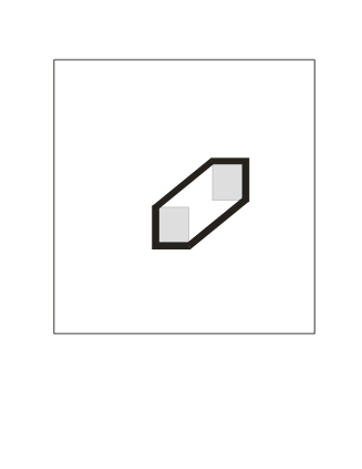
Figure 1. Geometry of the test problem. Gray areas represent charge areas. Thick black line represents the convex envelope of charge areas. Thin gray line represents the boundary $\Gamma$ of the domain $\Omega$.

It was found that if $P_{f}(\alpha,\Theta,\Psi)$ is calculated directly using the integration over $\Omega$, then the procedure based on (2.2.6) and (2.2.7) produces the convex hull of the charged areas with high accuracy. However, when $P_{f}(\alpha,\Theta,\Psi)$ is calculated using the integration over the boundary, the algorithm based on (2.2.6) produces the convex hull occupying the whole $\Omega$. Such a drastic difference is the result of small numerical errors in the boundary conditions determined by the numerical solution of the direct problem, and also in the numerical integration over the boundary.

Strong sensitivity to numerical errors arises from a specific nature of exponential functions. When $\alpha$ is large, these functions are rapidly increasing in one direction and rapidly oscillating in the orthogonal direction. As a result, small errors in boundary conditions are multiplied by large factors and the convex hull estimate based on (2.2.7) and (2.2.9) becomes distorted. For small values of $\alpha$, the value of $\log|P_{f}(\alpha,\Theta,\Psi)|/\alpha$ obtained using the integration over $\Omega$ is close to the one obtained using the integration over $\Gamma$. However, as $\alpha$ increases these two values diverge.

In order to verify the validity of the computational model, calculations were performed for the constant charge density: $f\equiv 1$ on $\Omega$. In this case, the precise value of $P_{f}(\alpha,\Theta,\Psi)$ can be computed analytically. For all values of $\alpha$, the analytical equations produced the same $\log|P_{f}(\alpha,\Theta,\Psi)|/\alpha$ values, no matter if the integration was performed over $\Omega$ or its boundary $\Gamma$. However, in the numerical analysis of this problem, the area and boundary integration were producing close values for small values of $\alpha$ and were diverging for large $\alpha$.

In practical problems based on experimental data, boundary conditions are always obtained with some errors. Therefore, as the above analysis show, in order to produce an algorithm for the solution of the inverse electrostatics problem that is numerically implementable, one needs to modify our approach. One possibility would be to find a set of harmonic functions exhibiting good behavior from the numerical viewpoint, which could replace the exponentials in the proof of Theorem 1.3.1.

3. Necessary and sufficient conditions for uniqueness of solutions

3.1. Proofs of uniqueness criteria

The goal of this subsection is to prove Theorems 1.2.2 and 1.2.6. Let us start with Theorem 1.2.2. To prove necessity, suppose that $u$ is a solution of problem (1.2.1) and let $h\in H(\Omega)$. Then

$$\int_{\Omega}f\cdot h=\int_{\Omega}\Delta u\cdot h=\int_{\Omega}u\cdot\Delta h=0.$$

Note that the boundary terms in the integration by parts disappear since $\phi_{1}=\phi_{2}=0$.

To prove sufficiency, denote by $G_{1}(x,y)$ the Green’s function of the Dirichlet boundary value problem in $\Omega$:

$$\Delta_{x}G_{1}(x,y)=\delta(x-y),\,\,\,G_{1}(x,y)|_{x\in\partial\Omega}=0,$$

and by $G_{2}(x,y)$ the Green’s function for the corresponding Neumann boundary value problem:

$$\Delta_{x}G_{2}(x,y)=\delta(x-y)-\frac{1}{|\Omega|},\,\,\,(\operatorname{grad}_{x}G_{2}(x,y),\nu)|_{x\in\partial\Omega}=0.$$

Note that the integral over $\Omega$ of the right–hand side of the equation above is zero, which is necessary for the existence of a solution of the Neumann problem with zero boundary conditions.

It follows from the definitions of $G_{1}$ and $G_{2}$ that

$$(G_{1}-G_{2})(x,y)+\frac{x_{1}^{2}}{2|\Omega|}$$

is a harmonic function of $x$. Therefore, the assumption $f\in Z$ implies

$$u(y):=\int_{\Omega}f(x)G_{1}(x,y)\,dx=\int_{\Omega}f(x)G_{2}(x,y)\,dx-\int_{\Omega}f(x)\frac{x_{1}^{2}}{2|\Omega|}\,dx$$

for all $y\in\Omega$. Note that the term

$$\int_{\Omega}f(x)\frac{x_{1}^{2}}{2|\Omega|}\,dx$$

is constant and hence of no importance for the Neumann boundary value problem. Let us also remark that $\int_{\Omega}f(x)dx=0$ since $f\in Z(\Omega)$. It is easy to check that, by the properties of $G_{1}$ and $G_{2}$, the function $u$ constructed above is a solution of problem (1.2.1). This completes the proof of Proposition 1.2.2. ∎

The proof of Theorem 1.2.6 is completely analogous. We note that the existence of Green’s functions for the Navier equation with either Dirichlet or Neumann boundary conditions is well-known — see, for instance [So, section 7.12].

3.2. Proof of Theorem 1.5.1

Proof of (i). Let $A,B,S$ be three spherical layers centered at the origin such that $A\cup B=S$ and $A~{}\cap~{}B=~{}\emptyset$. Consider the following linear combination of characteristic functions of the sets $A$ and $B$:

$$u=\operatorname{Vol}(B)\,\chi_{A}-\operatorname{Vol}(A)\,\chi_{B}.$$

By the mean value theorem for harmonic functions we immediately have $u\in Z(S)$, and this completes the proof of part (i) of the proposition.

Proof of (ii) In order to prove the second part of the proposition we note that a function $U$ lying in the kernel of the Navier operator $\mathcal{L}$ is biharmonic. Indeed, let $\mathcal{L}(U)=\Delta U+\alpha\operatorname{grad}\,\operatorname{div}U=0$. Taking the divergence on both sides we get $\operatorname{div}(\Delta U)=0$. Here we took into account that $\operatorname{div}\operatorname{grad}=\Delta$ and that the Laplacian commutes with the divergence. At the same time, applying the Laplacian to $\mathcal{L}(U)$ we get

$$\Delta^{2}\,U+\alpha\Delta\,\operatorname{grad}\,\operatorname{div}U=0.$$

But since $\operatorname{div}(\Delta U)=0$, the second term vanishes, because

$$\Delta\,\operatorname{grad}\,\operatorname{div}U=\operatorname{grad}\,\operatorname{div}\,\Delta U.$$

Hence, $\Delta^{2}U=0$ and $U$ is biharmonic.

It is well-known that a real valued biharmonic function $f(x)$ satisfies the following mean-value property (see, for example, [EK]):

$$\int_{B(x,r)}f(y)dy=\omega_{n}r^{n}f(x)+\frac{\omega_{n}\,r^{n+2}}{2(n+2)}\Delta f(x),$$ (3.2.1)

where $B(x,r)$ is a ball of radius $r$ centered at $x\in{\mathbb{R}}^{n}$ and $\omega_{n}$ is the volume of the unit ball in $\mathbb{R}^{n}$.

Consider now a ball $B=B(r_{3})$ centered at the origin. Let us represent it as a union of three sets $B(r_{1})\cup S(r_{1},r_{2})\cup S(r_{2},r_{3})$, $r_{3}>r_{2}>r_{1}>0$. Let $F_{a,b}$ be a piecewise constant vector-valued function taking the values $a$ and $b$ on $S(r_{2},r_{3})$ and $S(r_{1},r_{2}$), respectively, and the value one on $B(r_{1})$. Clearly, $F_{a,b}\in V_{\sigma}$ for all $a,b\in{\mathbb{R}}$. Let us show that for any triple $0<r_{1}<r_{2}<r_{3}$ there exists a choice of parameters $a,b$ such that $F_{a,b}\in\mathcal{Z}(B)$. It can be deduced from the mean-value formula (3.2.1), that the inclusion $F_{a,b}\in\mathcal{Z}(B)$ holds if the following system of equations is satisfied:

$$a(r_{3}^{n}-r_{2}^{n})+b(r_{2}^{n}-r_{1}^{n})+r_{1}^{n}=0,\,\,a(r_{3}^{n+2}-r_{2}^{n+2})+b(r_{2}^{n+2}-r_{1}^{n+2})+r_{1}^{n+2}=0.$$

One may check that the determinant of this system does not vanish for $r_{3}>r_{2}>r_{1}>0$. Indeed, if $r_{3}\neq r_{2}$, the only positive roots of the determinant considered as a polynomial in $r_{1}$ are $r_{1}=r_{2}$ and $r_{1}=r_{3}$ (there are no other positive roots because, as can be easily verified, the derivative with respect to $r_{1}$ has only one positive root). Hence, there always exists a unique solution $a,b$ of the system above, and the corresponding function $F_{a,b}\in\mathcal{Z}(B)$.

This completes the proof of Theorem 1.5.1.

Remark 3.2.2.

The proof of part (i) of Theorem 1.5.1 shows that the intersection $V_{\sigma}(S)\cap\mathcal{Z}(S)$ is in fact quite large. Indeed, it is easy to show that for any partition of $S$ into $k$ concentric spherical layers, there exists a $(k-1)$–dimensional linear subspace of functions in $V_{\sigma}\cap\mathcal{Z}(S)$.

The proof of part (ii) goes through without changes if instead of a ball $B(r_{3})$ one takes a spherical layer $S=S(r_{3},r_{0})=S(r_{0},r_{1})\cup S(r_{1},r_{2})\cup S(r_{2},r_{3})$. It follows from the proof that for any partition of $S$ into $k$ concentric spherical layers, there exists a $(k-2)$–dimensional linear space of functions in $\mathcal{V}_{\sigma}\cap\mathcal{Z}(S)$.

Acknowledgments

The authors are grateful to Victor Isakov and Leonid Polterovich for useful discussions. Research of Leonid Parnovski is supported by EPSRC grant EP/F029721/1. Research of Iosif Polterovich is supported by NSERC, FQRNT and Canada Research Chairs program.

References

- [AMR] G. Alessandrini, A. Morassi and E. Rosset, Detecting an inclusion in an elastic body by boundary measurements, SIAM J. Math. Anal. 33 No. 6 (2002), 1247–1268.
- [Ba] K.-J.Bathe, Finite Element Procedures in Engineering Analysis, Prentice-Hall, 1982.
- [Ca] A.P. Calderón, On an inverse boundary value problem, in Seminar on Numerical Analysis and its Applications to Continuum Physics, Rio de Janeiro, Editors W.H. Meyer and M.A. Raupp, Sociedade Brasileira de Matematica, (1980). 65-73.
- [CS] M.V.K. Chari and S.J. Salon, Numerical Methods in Electromagnetism, Academic Press, 2000.
- [CRS] T.C. Chu, W.F. Ranson, and M.A. Sutton, Applications of digital-image-correlation techniques to experimental mechanics, Experimental Mechanics Vol. 25 (1985) p. 232.
- [BSB] L. Ballani, D. Stromeyer, F. Barthelmes, Decomposition principles for linear source problems. In: Inverse Problems: Principles and Applications in Geophysics, Technology and Medicine. Anger, G. et al, eds., Mathematical Research, Vol. 74, Akademie-Verlag, Berlin 1993, p. 45-59.
- [BSD] D. Ban, E.H. Sargent, St.J. Dixon-Warren, G. Lethal, K. Hinzer, J.K. White, and D.G. Knight, Scanning Voltage Microscopy on Buried Heterostructure Multiquantum-Well Lasers: Identification of a Diode Current Leakage Path, IEEE Journal of Quantum Electronics, Vol. 40 (2004), 118–122.
- [Du] D.G. Duffy, Transform Methods for Solving Partial Differential Equations, Chapman Hall/CRC, 2004.
- [EK] M. El Kadiri, Sur la propriété de la moyenne restreinte pour les fonctions biharmoniques, C. R. Acad. Sci. Paris, Ser. I 335 (2002) 427–429.
- [GAT] A. Gruverman, O. Auciello, and H. Tokumoto, Scanning Force Microscopy: Application to Nanoscale Studies of Ferroelectric Domains, Integrated Ferroelectrics, Vol. 19 (1998) p. 49.
- [Hi] F.B. Hildebrand, Finite-Difference Equations and Simulations, Prentice-Hall, 1968.
- [Is1] V. Isakov, Inverse Source Problems, Math. Surveys and Monographs 34, Amer. Math. Soc., 1990.
- [Is2] V. Isakov, Inverse Problems for Partial Differential Equations, Springer-Verlag, 2006.
- [Is3] V. Isakov, Inverse obstacle problems, Inverse Problems 25 (2009) 123002.
- [Ja] J.D. Jackson, Classical Electrodynamics , John Wiley and Sons, 1999.
- [Kh] A.G. Khachaturyan, Theory of Structural transformations in Solids, John Wiley Sons, New York, 1983.
- [KBS] S.B. Kuntze, D. Ban, E.H. Sargent, St. J. Dixon-Warren, and J.K. White and K. Hinzer, Electrical Scanning Probe Microscopy: Investigating the Inner Workings of Electronic and Optoelectronic Devices, Critical Reviews in Solid State and Materials Sciences Vol. 30 ( 2005) p. 71.
- [LK] A. Leyk and E. Kubalek, MMIC Internal Electric Field Mapping with Submicrometre Spatial Resolution and Gigahertz Bandwidth by Means of High Frequency Scanning Force Microscope Testing, Electronic Letters, Vol. 31 (1995), p. 2089.
- [MiFo] V. Michel and A.S. Fokas, A unified approach to various techniques for the non-uniqueness of the inverse gravimetric problem and wavelet-based methods, Inverse Problems 24 (2008) 045019.
- [MG] A.R. Mitchell and D.F. Griffiths, The Finite Difference Method in Partial Differential Equations, John Wiley Sons, 1980.
- [MoFe] P.M. Morse and H. Feshbach, Methods of Theoretical Physics, McGraw-Hill Book Company, 1953.
- [NU] G. Nakamura and G. Uhlmann, Global uniqueness for an inverse boundary problem arising in elasticity, Invent. Math. 118 (1994), 457–474.
- [Pr] M.B. Prime, Cross-Sectional Mapping of Residual Stresses by Measuring the Surface Contour After a Cut, Transactions of the ASME, Vol. 123 (2001) p. 163
- [Sa] M.N.O. Sadiku, Numerical Techniques in Electromagnetics, CRC Press, 1992.
- [So] L. Solomon, Élasticité linéaire, Masson et Cie, Paris, 1968.
- [St] J.C. Strikwerda, Finite Difference Schemes and Partial Differential Equations, SIAM, 2004.
- [TG] S.P. Timoshenko and J.N. Goodier, Theory of Elasticity, McGraw-Hill Book Company, 1970.
- [Ts] C.C. Tschering, Density-gravity covariance functions produced by overlapping rectangular blocks of constant density, Geophys. J. Int. 105 (1991), 771-776.
- [Uh] G. Uhlmann, Electrical impedance tomography and Calderón’s problem, Inverse Problems 25 (2009), no. 12, 123011.
- [Wi1] P.J. Withers, Handbook of Residual Stress Analysis, Society of Experimental Mechanics, 1997.
- [Wi2] P.J. Withers, Residual stress and its role role in failure, Reports on progress in physics, Vol. 70 (2007) p. 2211.
- [XCS] Y. Xie, J. Cong and S. Sapatnekar (Editors), Three-Dimensional Integrated Circuit Design. EDA, Design and Microarchitectures, Springer, New York, 2010.