Kinetic theory of nonequilibrium stochastic long-range systems: Phase transition and bistability

Abstract

We study long-range interacting systems driven by external stochastic forces that act collectively on all the particles constituting the system. Such a scenario is frequently encountered in the context of plasmas, self-gravitating systems, two-dimensional turbulence, and also in a broad class of other systems. Under the effect of stochastic driving, the system reaches a stationary state where external forces balance dissipation on average. These states have the invariant probability that does not respect detailed balance, and are characterized by non-vanishing currents of conserved quantities. In order to analyze spatially homogeneous stationary states, we develop a kinetic approach that generalizes the one known for deterministic long-range systems; we obtain a very good agreement between predictions from kinetic theory and extensive numerical simulations. Our approach may also be generalized to describe spatially inhomogeneous stationary states. We also report on numerical simulations exhibiting a first-order nonequilibrium phase transition from homogeneous to inhomogeneous states. Close to the phase transition, the system shows bistable behavior between the two states, with a mean residence time that diverges as an exponential in the inverse of the strength of the external stochastic forces, in the limit of low values of such forces.

1 Introduction

Systems of particles interacting through two-body non-integrable potentials, also called long-range interactions, abound in nature. Common examples are plasmas interacting through repulsive or attractive Coulomb potential, self-gravitating systems (globular clusters, galaxies) involving interaction through attractive Newton potential, two-dimensional turbulence, and many others. In addition, there are several model systems with non-integrable interactions which have been studied extensively in recent years, such as spins, vortices in two dimensions, etc [1, 2, 3, 4, 5].

Very often, these systems are acted upon by external stochastic forces that drive them out of equilibrium. Unlike systems with short-range interactions, stochastic forces in long-range interacting systems act coherently on all particles, and not independently on each particle. Consider, e.g., globular clusters being influenced by the gravitational potential of their galaxy, which produces a force that fluctuates along their physical trajectories. In addition, galaxies themselves feel the random potential of other surrounding galaxies, and their halos are subjected to transient and periodic perturbations, which may be due to the passing of dwarfs or to orbital decaying [6]. Dynamics of plasmas are also strongly influenced by fluctuating electric and magnetic fields due to the ever-changing ambiance [7]. In situations of stochastic driving, the systems at long times often reach a nonequilibrium stationary state that violates detailed balance. In such a state, the power injected by the external random fields balances on average the dissipation, and there is a steady flux of conserved quantities through the system.

Study of nonequilibrium stationary states (NESS) is an active area of research of modern day statistical mechanics. One of the primary challenges in this field is to formulate a tractable framework to analyze nonequilibrium systems on a common footing, similar to the one due to Gibbs and Boltzmann that has been established for equilibrium systems [9, 10, 8]. This paper provides, to our knowledge, the first study of NESS in long-range systems with statistical mechanical perspectives.

Common theoretical approaches to study isolated systems with long-range interactions include the kinetic theory description of relaxation towards equilibrium. In plasma physics and astrophysics, this approach leads to the Lenard-Balescu equation or to the approximate Landau equation [11, 12]. One of the main theoretical results of this paper is a detailed development of a generalization of this kinetic theory approach to describe nonequilibrium stationary states in systems with long-range interactions driven by external stochastic forces, valid in the limit of small external stochastic fields. The nonequilibrium kinetic equation that we obtain describes the temporal evolution of the one-particle distribution function. In the limit of small external forcing, the system settles into a stationary state, in which we find the one-particle momentum distribution to be non-Gaussian. The predictions of our kinetic equation for spatially homogeneous stationary states compare very well with results of our extensive $N$-particle numerical simulations on a paradigmatic model of long-range interacting systems. Our numerical simulations also exhibit a nonequilibrium phase transition between homogeneous and inhomogeneous states. Close to the phase transition, we demonstrate the occurrence of bistability between these two types of states, with a mean residence time that diverges as an exponential in the inverse of the strength of the external forcing, in the limit of low values of such forcing.

Similar bistable behavior has recently been observed in two-dimensional turbulence with stochastic forcing [13]. We believe that such phase transitions are essential phenomena for geophysical flows and climate, for which the two-dimensional Euler equations are a simplified paradigmatic model. There exists a very strong analogy between the two-dimensional Euler equations and the Vlasov equation relevant for leading order dynamics of the model we discuss in this paper [14, 15]. One of the motivations of the present work is to be able to study analogous phenomena in a setup for which the theory can be more easily worked out.

In a recent letter, we reported on some of the above findings, in one of the first studies of non-equilibrium stationary states in systems with non-integrable potentials and driven by external stochastic fields [16]. The aim of this paper is to present a detailed derivation of the results given in Ref. [16], as well as to report on additional empirical results, more specifically non-equilibrium phase transitions.

We note that Ref. [17] presents a computation of the same kinetic equation as the one we describe in this work and in [16]. Nevertheless, the result is different.

The structure of the paper is as follows. In the following section, we define the dynamics we are going to consider of a long-range interacting system driven by external stochastic forces. We also discuss the paradigmatic example of the Hamiltonian mean-field (HMF) model. In section 3, we discuss the methods we adopt to analyze the dynamics. In particular, we give a detailed derivation of the kinetic theory to study spatially homogeneous stationary states of the dynamics. We describe the numerical simulation scheme that we employ to study the dynamics, specifically, to check the predictions of our kinetic theory. This is followed by a discussion in section 4 of the results obtained from the kinetic theory, and their comparison with numerical simulation results for spatially homogeneous stationary states. In section  5, we discuss the results of numerical simulations of spatially inhomogeneous stationary states. We report on the very interesting bistable behavior in which the system in the course of its temporal evolution switches back and forth between homogeneous and inhomogeneous states, with a mean residence time that we show to be diverging as an exponential in the inverse of the strength of the external stochastic forcing, in the limit of low values of such forcing. We close the paper with concluding remarks. Some of the technical details of our computation are collected in the four appendices.

2 Long-range interacting systems driven by stochastic fields

2.1 The model

Consider a system of $N$ particles interacting through a long-range pair potential, and described by the Hamiltonian

$$H=\sum_{i=1}^{N}\frac{p_{i}^{2}}{2}+\frac{1}{2N}\sum_{i,j=1}^{N}v(q_{i}-q_{j}).$$ (1)

Here, $q_{i}$ and $p_{i}$ are, respectively, the coordinate and the momentum of the $i$-th particle, and $v(q)$ is the two-body interaction potential. We take the particles to be of unit mass. In this paper, for simplicity, we regard $q_{i}$’s as scalar periodic variables of period $2\pi$; generalization to $q_{i}\in\mathbb{R}^{n}$, with $n=1,2$ or $3$, is straightforward.

In plasma physics, the typical number of particles interacting with one particle is given by the coupling parameter $\Gamma=n\lambda_{D}^{3}$, where $n$ is the number density, and $\lambda_{D}$ is the Debye length. It is then usual to rescale time such that the inverse of $\Gamma$ multiplies the interaction term [11]. In self-gravitating systems, the dynamics is dominated by collective effects, so that it is natural to rescale time in such a way that the parameter $1/N$ multiplies the interaction potential [18]. These facts explain the rescaling of the potential energy by $1/N$ in Eq. (1), called the Kac scaling in systems with long-range interactions [19]. We emphasize that no generality is lost in adopting the Kac prescription.

We perturb the system (1) by a statistically homogeneous Gaussian stochastic field $F(q,t)$ with zero mean, and variance given by

$$\langle F(q,t)F(q^{\prime},t^{\prime})\rangle=C(|q-q^{\prime}|)\delta(t-t^{\prime}).$$ (2)

The resulting equations of motion for the $i$-th particle are

$$\dot{q}_{i}=\frac{\partial H}{\partial p_{i}},\qquad{\rm and}\qquad\dot{p}_{i}=-\frac{\partial H}{\partial q_{i}}-\alpha p_{i}+\sqrt{\alpha}\,F(q_{i},t).$$ (3)

The property that the Gaussian fields $F(q_{i},t)$ are statistically homogeneous, i.e., the correlation function $C$ depends solely on $|q-q^{\prime}|$, is consistent with any perturbation that respects space homogeneity. Such a property is necessary for the discussions later in the paper on the kinetic theory approach to describe spatially homogeneous stationary states of the dynamics (3). Note that $C(q)$ is the correlation, so that it is a positive-definite function [20], and its Fourier components are positive:

$$c_{k}\equiv\frac{1}{2\pi}\int_{0}^{2\pi}{\rm d}q\leavevmode\nobreak\ C(q)e^{-ikq}>0;\leavevmode\nobreak\ \leavevmode\nobreak\ c_{-k}=c_{k},\leavevmode\nobreak\ \leavevmode\nobreak\ \leavevmode\nobreak\ \leavevmode\nobreak\ C(q)=c_{0}+2\sum_{k=1}^{\infty}c_{k}\cos(kq).$$ (4)

We find it convenient to use the equivalent Fourier representation of the Gaussian field $F(q,t)$ as follows:

$$F(q,t)\,=\,\sqrt{c_{0}}\ X_{0}(t)+\sum_{k=1}^{\infty}\sqrt{2c_{k}}\left[\cos(kq)\,X_{k}(t)+\sin(kq)\,Y_{k}(t)\right],$$ (5)

where $X_{0}(t)$, $X_{k}(t)$ and $Y_{k}(t)$ are independent scalar Gaussian white noises satisfying

$$\langle X_{k}(t)\,X_{k^{\prime}}(t^{\prime})\rangle=\delta_{k,k^{\prime}}\delta(t-t^{\prime}),$$ (6)

$$\langle Y_{k}(t)\,Y_{k^{\prime}}(t^{\prime})\rangle=\delta_{k,k^{\prime}}\delta(t-t^{\prime}),$$ (7)

$$\langle X_{k}(t)\,Y_{k^{\prime}}(t^{\prime})\rangle=0.$$ (8)

For stochastic dynamics of the type Eq. (3), general mathematical results allow to prove that the dynamics is ergodic (see, for instance, [21]).

Using the Itō formula [22] to compute the time derivative of the energy density $e=H/N$, and averaging over noise realizations give

$$\left\langle\frac{de}{dt}\right\rangle+\left\langle 2\alpha\kappa\right\rangle=\frac{\alpha}{2}C(0),$$ (9)

where $\kappa=\sum_{i=1}^{N}p_{i}^{2}/(2N)$ is the kinetic energy density. On integration, we get for homogeneous states for which $e=\kappa$ that

$$\langle k(t)\rangle\,=\,\left(\langle k(0)\rangle-\frac{C(0)}{4}\right)\,e^{-2\alpha t}\,+\,\frac{C(0)}{4}.$$ (10)

The average kinetic energy density in the stationary state is thus $\left\langle\kappa\right\rangle_{ss}=C(0)/4$. We define the kinetic temperature of the system as

$$\left\langle\kappa\right\rangle_{ss}\equiv\frac{T}{2};$$ (11)

as a result, we have

$$T=\frac{C(0)}{2}.$$ (12)

Let us note that in the dynamics (3), fluctuations of intensive observables due to stochastic forcing are of order $\sqrt{\alpha}$, while those due to finite-size effects are of order $1/\sqrt{N}$. Moreover, the typical timescale associated with the effect of stochastic forces is $1/\alpha$, as is evident from Eq. (10), while the one associated with relaxation to equilibrium due to finite-size effects is of order $N$, see [1, 2].

Our theoretical analysis to study the dynamics (3) by means of kinetic theory is valid for any general two-particle interaction potential $v(q)$. However, in order to perform simple numerical simulations with which we may check the predictions of the kinetic theory, we specifically make the choice $v(q)=1-\cos q$, that defines the stochastically-forced attractive Hamiltonian mean-field (HMF) model, as detailed below.

2.2 A specific example: The stochastically-forced HMF model

The Hamiltonian mean-field (HMF) model is a paradigmatic model to study long-range interacting systems. The model describes particles moving on a circle under deterministic Hamiltonian dynamics, and interacting through the interparticle potential $v(q)=1-\cos q$ [24, 23]. It displays many features of generic long-range interacting systems, e.g., existence of quasistationary states [24, 1]. In equilibrium, the model has a second-order phase transition from a high-energy spatially homogeneous phase to a low-energy inhomogeneous phase at the energy density $e_{c}=3/4$, corresponding to the critical temperature $T_{c}=1/2$. In a system of $N$ particles, the degree of spatial inhomogeneity at time $t$ is measured by the magnetization variable $m(t)$, defined as

$$m(t)=\frac{1}{N}\sqrt{\Big{(}\sum_{i=1}^{N}\cos q_{i}\Big{)}^{2}+\Big{(}\sum_{i=1}^{N}\sin q_{i}\Big{)}^{2}}.$$ (13)

In the thermodynamic limit $N\to\infty$, the magnetization in the steady state decreases continuously as a function of energy from one to zero at the transition energy $e_{c}$, and remains zero at all higher energies. When forced by the stochastic forces $F(q_{i},t)$ resulting in the dynamics (3), we call the corresponding model the stochastically-forced HMF model. We note for later purpose that the Fourier transform of the HMF interparticle potential is, for $k\neq 0$, $v_{k}=-\left[\delta_{k,1}+\delta_{k,-1}\right]/2$, where $\delta_{k,i}$ is the Kronecker delta.

3 Methods of analysis

3.1 Kinetic theory for homogeneous stationary states

Here, we develop a suitable kinetic theory description to study the dynamics (3) in the joint limit $N\to\infty$ and $\alpha\to 0$. While the first limit is physically motivated on grounds that most long-range systems indeed contain a large number of particles, the second one allows us to study stationary states for small external forcing. Moreover, for small $\alpha$, we will be able to develop a complete kinetic theory for the dynamics. For simplicity, we discuss here the continuum limit $N\alpha\gg 1$, when stochastic effects are predominant with respect to finite-size effects. The generalization of the following discussion to the cases $N\alpha$ of order one and $N\alpha\ll 1$ is straightforward, as pointed out at the end of this subsection. For the development of the kinetic theory, we assume the system to be spatially homogeneous; a possible generalization to the non-homogeneous case will be discussed in the conclusions of the paper.

As a starting point to develop the theory, we consider the Fokker-Planck equation associated with the equations of motion (3). This equation describes the evolution of the $N$-particle distribution function $f_{N}(q_{1},...,q_{N},p_{1},...,p_{N},t)$, which is the probability density (after averaging over noise realizations) to observe the system with coordinates and momenta around the values $\{q_{i},p_{i}\}_{1\leq i\leq N}$ at time $t$. This equation can be derived by standard methods [22]; we have

$$\frac{\partial f_{N}}{\partial t} = \sum_{i=1}^{N}\left[-p_{i}\frac{\partial f_{N}}{\partial q_{i}}+\frac{\partial(\alpha p_{i}f_{N})}{\partial p_{i}}\right]+\frac{1}{2N}\sum_{i,j=1}^{N}\frac{\partial v(q_{i}-q_{j})}{\partial q_{i}}\left[\frac{\partial}{\partial p_{i}}-\frac{\partial}{\partial p_{j}}\right]f_{N}$$ (14)

$$+\frac{\alpha}{2}\sum_{i,j=1}^{N}C(|q_{i}-q_{j}|)\frac{\partial^{2}f_{N}}{\partial p_{i}\partial p_{j}}.$$

In A, by applying the so-called potential conditions [25] for the above Fokker-Planck equation, we prove that a necessary and sufficient condition for the stochastic process (3) to verify detailed balance is that the Gaussian noise is white in space, that is, $c_{k}=c$ for all $k$. This condition is not satisfied for a generic correlation function $C(q)$, in which case, the steady states of the dynamics are true nonequilibrium ones, characterized by non-vanishing probability currents in configuration space, and a balance between external forces and dissipation.

Similar to the Liouville equation for Hamiltonian systems, the $N$-particle Fokker-Planck equation (14) is a very detailed description of the system. Using kinetic theory, we want to describe the evolution of the one-particle distribution function

$$f(z_{1},t)=\int\prod_{i=2}^{N}\,{\rm d}z_{i}f_{N}(z_{1},...,z_{N},t),$$ (15)

where we have used the notation $z_{i}\equiv(q_{i},p_{i})$. We note that with this definition, the normalization is $\int{\rm d}zf(z,t)=1$. Substituting in the Fokker-Planck equation (14) the reduced distribution functions

$$f_{s}(z_{1},...,z_{s},t)=\frac{N!}{(N-s)!N^{s}}\int\prod_{i=s+1}^{N}\,{\rm d}z_{i}\,f_{N}(z_{1},...,z_{N},t),$$ (16)

and using standard techniques [26], we get a hierarchy of equations, similar to those of the Bogoliubov-Born-Green-Kirkwood-Yvon (BBGKY) hierarchy, as follows:

$$\frac{\partial f_{s}}{\partial t}+\sum_{i=1}^{s}p_{i}\frac{\partial f_{s}}{\partial q_{i}}-\frac{1}{N}\sum_{i,j=1}^{s}\frac{\partial v(q_{i}-q_{j})}{\partial q_{i}}\frac{\partial f_{s}}{\partial p_{i}}-\sum_{i=1}^{s}\frac{\partial}{\partial p_{i}}[\alpha p_{i}f_{s}]$$

$$-\frac{\alpha}{2}\sum_{i,j=1}^{s}C(|q_{i}-q_{j}|)\frac{\partial^{2}f_{s}}{\partial p_{i}\partial p_{j}}=\sum_{i=1}^{s}\int dz_{s+1}\frac{\partial}{\partial q_{i}}v(q_{i}-q_{s+1})\frac{\partial f_{s+1}}{\partial p_{i}}$$ (17)

for $s=1,...,N-1$. In this paper, we use both the notations $\partial h/\partial q$ and $h^{\prime}$ to denote the derivative of a function $h$. With a slight abuse of the standard vocabulary, we will refer to Eq. (3.1) as the BBGKY hierarchy equation.

Now, as is usual in kinetic theory, we split the reduced distribution functions into connected and non-connected parts, e.g.,

$$f_{2}(z_{1},z_{2},t)=f(z_{1},t)f(z_{2},t)+\tilde{g}(z_{1},z_{2},t),$$ (18)

and similarly, for other $f_{s}$’s with $s>2$. In B, we show that the connected part $\tilde{g}(z_{1},z_{2},t)$ of the two-particle correlation is of order $\alpha$, so that we may write

$$f_{2}(z_{1},z_{2},t)=f(z_{1},t)f(z_{2},t)+\alpha g(z_{1},z_{2},t),$$ (19)

where $g$ is of order unity; more generally, the connected part of the $k$-particle correlation is of higher order, with respect to $\alpha$, in the small parameters $\alpha$ and $1/N$. Then, to close the BBGKY hierarchy, we neglect the effect of the connected part of the three-particle correlation on the evolution of the two-particle correlation function. This scheme is justified at leading order in the small parameter $\alpha$, and is the simplest self-consistent closure scheme for the hierarchy while taking into account the effects of the stochastic forcing. With our assumption that the system is homogeneous, i.e., $f$ depends on $p$, and $g$ depends on $|q_{1}-q_{2}|$, $p_{1}$ and $p_{2}$ only, the first two equations of the hierarchy are then

$$\frac{\partial f}{\partial t}-\alpha\frac{\partial}{\partial p}[pf]-\frac{\alpha}{2}C(0)\frac{\partial^{2}f}{\partial p^{2}}=\alpha\frac{\partial}{\partial p}\int{\rm d}q_{1}{\rm d}p_{1}v^{\prime}(q_{1})g(q_{1},p,p_{1},t),$$ (20)

and

$$\frac{\partial g}{\partial t}+L_{f}^{(1)}g+L_{f}^{(2)}g = C(|q_{1}-q_{2}|)f^{\prime}(p_{1},t)f^{\prime}(p_{2},t),$$ (21)

where $L_{f}^{(1)}$ and $L_{f}^{(2)}$ are the Vlasov operators linearized about the one-particle distribution $f$, and acting, respectively, on the first pair $(q_{1},p_{1})$ and on the second pair $(q_{2},p_{2})$ of the function $g=g(q_{1},p_{1},q_{2},p_{2},t)$. Explicitly, for a function $h$ of $(q,p,t)$, the expression for the linear Vlasov operator $L_{f}h$ is

$$L_{f}h(q,p,t)=p\frac{\partial h}{\partial q}-f^{\prime}(p,t)\int{\rm d}q_{1}{\rm d}p_{1}\,v^{\prime}(q-q_{1})h(q_{1},p_{1},t),$$ (22)

so that we have for $L_{f}^{(1)}g$,

$$L_{f}^{(1)}g(q_{1}-q_{2},p_{1},p_{2},t)=p_{1}\frac{\partial g}{\partial q_{1}}-f^{\prime}(p_{1},t)\int{\rm d}q_{3}{\rm d}p_{3}\,v^{\prime}(q_{1}-q_{3})g(q_{3}-q_{2},p_{3},p_{2},t).$$

$L_{f}^{(2)}g$ is obtained from Eq. (3.1) by exchanging the subscripts $1$ and $2$.

To obtain from Eqs. (20) and (21) a single kinetic equation for the distribution function $f$, we have to solve Eq. (21) for $g$ as a function of $f$ and plug the result into the right hand side of Eq. (20). Because the two equations are coupled, this program is not achievable without making further simplifying assumption. Nevertheless, we readily see from these equations that the two-particle correlation $g$ evolves over a timescale of order one, whereas the one-particle distribution function $f(p,t)$ evolves over a timescale of order $1/\alpha$. We may then use this timescale separation and compute the long-time limit of $g$ from Eq. (21) by assuming $f$ to be steady in time; this is the equivalent of the Bogoliubov’s hypothesis in the kinetic theory for isolated systems with long-range interactions. Note that for this timescale separation to be valid, we must also suppose that the one-particle distribution function $f(p,t)$ is a stable solution of the Vlasov equation at all times. Indeed, if this is not the case, it can be shown that $g$ diverges in the limit $t\to\infty$ [27]. The physical content of this hypothesis is that the system slowly evolves from the initial condition through a sequence of quasistationary states to the final stationary state.

Because we assume the system to be homogeneous in space, it is useful to Fourier transform Eqs. (20) and (21) with respect to the spatial variable; we get

$$\frac{\partial f}{\partial t}-\alpha\frac{\partial}{\partial p}[pf]-\frac{\alpha}{2}C(0)\frac{\partial^{2}f}{\partial p^{2}}=-2\pi i\alpha\sum_{k=-\infty}^{\infty}kv_{k}\frac{\partial}{\partial p}\int\mathrm{d}p^{\prime}\,g_{k}(p,p^{\prime},t),$$ (24)

and

$$\left(\frac{\partial g_{k}}{\partial t}+L_{f,k}^{(1)}g_{k}+L_{f,-k}^{(2)}g_{k}\right)(p_{1},p_{2},t)=c_{k}f^{\prime}(p_{1})f^{\prime}(p_{2}),$$ (25)

where $g_{k}(p_{1},p_{2},t)$ is the Fourier transform of $g(q,p_{1},p_{2},t)$ with respect to the spatial variable, and $v_{k}$ is the $k$-th Fourier coefficient of the pair potential $v(q)$. The explicit expression for the $k$-th Fourier component of the linear Vlasov operator $L_{f,k}$ acting on a function $h(p)$ is

$$\Bigl{(}L_{f,k}h\Bigr{)}(k,p)=ikph(p)-2\pi ikv_{k}f^{\prime}(p)\int\mathrm{d}p^{\prime}\,h(p^{\prime}).$$ (26)

One has analogous expressions for $L_{f,k}^{(1)}$ and for $L_{f,-k}^{(2)}$. We readily see that $L_{f,k}^{*}=L_{f,-k}$.

From the right hand side of Eq. (24), we see that to obtain a single kinetic equation, we need only the Fourier transform $g_{k}(p,p^{\prime},t)$, more specifically, its integral with respect to the second momentum variable $p^{\prime}$. Actually, it can be shown that $g_{k}(p,p^{\prime},t)$ does not have a well-defined time-asymptotic (it converges only in the sense of distribution), while its integral with respect to $p^{\prime}$ does have; this is connected to the mechanism of Landau damping [27].

The structure of Eqs. (20) and (21), or, equivalently, of Eqs. (24) and (25) is very familiar in kinetic theories; we refer the reader to [27] for a general discussion. Equation (21), or, equivalently, Eq. (25), is called the Lyapunov equation for the two-point correlation of a stochastic variable described by an Ornstein–Uhlenbeck process. However, there is a difference from the standard finite-dimensional case [22] in that in our case, $L_{f}$ is a linear infinite-dimensional operator acting on a functional space, instead of being a finite-dimensional one, i.e., a matrix. This makes it non-trivial to compute the long-time asymptotic of the right hand side of Eq. (20), where $g$ is the solution of Eq. (21) with $f$ steady in time. A possible way to achieve this goal is to follow the derivation of the Lenard–Balescu equation from the BBGKY hierarchy, as may be found in the Appendix A of Ref. [11]. For explicit technical details, see [27], in which the method to solve the Lyapunov equation in a general manner is discussed, and, subsequently, applied to the derivation of kinetic theories for long-range interacting systems and two-dimensional turbulence models.

In the present case, the linear transform of the stationary solution of the Lyapunov equation, Eq. (25), which is needed to compute the right hand side of Eq. (24), can be written (see Ref. [27]) in the frequency space as

$$\int dp_{1}\,g_{k}^{\infty}[f](p,p_{1}) \equiv \lim_{t\to\infty}\int dp_{1}\,g_{k}(p,p_{1},t)$$ (27)

$$= \frac{1}{\pi}\int_{\Gamma}\mathrm{d}\omega\,\Bigl{(}R_{f,k}(\omega)b\Bigr{)}(p)\,\int\mathrm{d}p^{\prime}\,\Bigl{(}R_{f,-k}(-\omega)b^{*}\Bigr{)}(p^{\prime}),$$ (28)

where $\Gamma$ is a contour which passes above all the poles of $\Bigl{(}R_{f,k}(\omega)b\Bigr{)}$, and $R_{f,k}(\omega)$ is the resolvent operator, defined as

$$R_{f,k}(\omega)\equiv(-i\omega+L_{f,k})^{-1},$$ (29)

while $b(p,t)=\sqrt{c_{k}}f^{\prime}(p,t)$. The discussion of the explicit form of the resolvent operator is a standard topic in plasma theory, and involves the phenomenon of Landau damping; we refer the reader to classical references for this result, for example, [28, 11, 12]. Its action on a function $h$, defined for $\omega$ such that $\mathrm{Im}(\omega)>0$, is

$$\Bigl{(}R_{f,k}(\omega)h\Bigr{)}(p)=\frac{1}{-i\omega+ikp}\left[h(p)+\frac{2\pi ikv_{k}}{\varepsilon(k,\omega)}f^{\prime}(p)\int\mathrm{d}p^{\prime}\,\frac{h(p^{\prime})}{-i\omega+ikp^{\prime}}\right],$$ (30)

where $\varepsilon(k,\omega)$ is the dielectric function, which for $\mathrm{Im}(\omega)>0$ is given by

$$\varepsilon(k,\omega)=\left[1-2\pi iv_{k}k\int{\rm d}p\frac{f^{\prime}(p)}{-i\omega+ikp}\right],$$ (31)

and by its analytic continuation for $\omega$ when $\mathrm{Im}(\omega)\leq 0$. Both the resolvent operator and the dielectric function are defined for $\omega\in\mathbb{R}$ by their analytic continuation, which will still be denoted by the same symbols.

Now, inserting Eq. (30) into Eq. (27), and with some calculations whose details will be reported in [27], we get the kinetic equation

$$\frac{\partial f}{\partial t}-\alpha\frac{\partial(pf)}{\partial p}-\alpha\frac{\partial}{\partial p}\left[D[f]\frac{\partial f}{\partial p}\right]=0,$$ (32)

where

$$D[f](p) = \frac{1}{2}C(0)$$ (33)

$$+2\pi\sum_{k=1}^{\infty}v_{k}c_{k}\int^{*}{\rm d}p_{1}\left[\frac{1}{|\varepsilon(k,kp)|^{2}}+\frac{1}{|\varepsilon(k,kp_{1})|^{2}}\right]\frac{1}{p_{1}-p}f^{\prime}(p_{1},t).$$

We recall that $v_{k}$ is the $k$-th Fourier coefficient of the pair potential $v(q)$, the quantity $c_{k}$ is defined in Eq. (4), $\varepsilon$ is the dielectric function defined in Eq. (31), and $\int^{*}$ indicates the Cauchy integral or Principal Value.

The kinetic equation (32) is the central result of the kinetic theory developed in this paper. It has the form of a non-linear Fokker-Planck equation [25] because the diffusion coefficient $D[f](p)$ is itself a functional of the one-particle distribution function $f$. The linear part of the diffusion coefficient $(1/2)C(0)$ is the mean-field effect of the stochastic forces, whereas the effect of two-particle correlation is encoded in the non-linear part. In the next section, we describe how we use this kinetic equation to get information about the nonequilibrium stationary states of the dynamics.

In the foregoing, we discussed the kinetic theory in the limit $N\alpha\gg 1$. The extension to the general case is straightforward: Because of the linearity of the equations of the hierarchy (20) and (21), the finite-$N$ and stochastic effects give independent contributions. The kinetic equation at leading order of both stochastic and finite-size effects is

$$\frac{\partial f}{\partial t}=Q_{\alpha}[f]+Q_{N}[f],$$ (34)

where $Q_{\alpha}$ is the operator described in Eq. (32), and $Q_{N}$ (of order $1/N$) is the Lenard-Balescu operator. For instance, in the case $N\alpha\ll 1$ and in dimensions greater than one, the operator $Q_{N}$ is responsible for the relaxation to Boltzmann equilibrium after a timescale of order $N$, whereas the smaller effect of $Q_{\alpha}$ selects the actual temperature after a longer timescale of order $1/\alpha$.

3.2 Numerical simulations

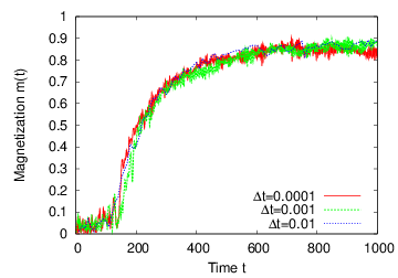
Figure 1: Magnetization as a function of time, obtained from numerical simulation of the stochastically-forced HMF model with $N=1000,\alpha=0.01$ at kinetic temperature $T=0.25$, and with $c_{1}=c_{2}=c_{3}=\ldots=c_{10}=C(0)/20,c_{k\geq 11}=0$, where $C(0)=2T$. The values of the integration step size $\Delta t$ used are marked in the figure. The data are obtained by using the integration algorithm described in section 3.2. That the magnetization plots collapse onto one curve shows the stability of our algorithm with respect to variation in $\Delta t$. We have checked that the final value of the magnetization matches with the prediction from equilibrium statistical mechanics.

Here we describe how we may simulate the dynamics (3) by means of a numerical integration scheme. To simulate the dynamics over a given time interval $[0:\mathcal{T}]$, choose a time step size $\Delta t$, and set $t_{n}=n\Delta t$ as the $n$-th time step of the dynamics. Here, $n=0,1,2,\ldots,N_{t}$, where $N_{t}=\mathcal{T}/\Delta t$. In our numerical scheme, at every time step, we first discard the effect of the noise and employ a fourth-order symplectic algorithm to integrate the deterministic Hamiltonian part of the dynamics [29]. Subsequently, we add the effect of noise and implement an Euler-like first-order algorithm to update the dynamical variables . Specifically, one step of the scheme from $t_{n}$ to $t_{n+1}=t_{n}+\Delta t$ involves the following updates of the dynamical variables for $i=1,2,\ldots,N$: For the symplectic part, we have, for $m=1,\ldots,4$,

$$p_{i}\Big{(}t_{n}+\frac{m\Delta t}{4}\Big{)}=p_{i}\Big{(}t_{n}+\frac{(m-1)\Delta t}{4}\Big{)}+b(m)\Delta t\Big{[}-\frac{\partial H}{\partial q_{i}}(\{q_{i}\Big{(}t_{n}+\frac{(m-1)\Delta t}{4}\Big{)}\})\Big{]},$$

$$q_{i}\Big{(}t_{n}+\frac{m\Delta t}{4}\Big{)}=q_{i}\Big{(}t_{n}+\frac{(m-1)\Delta t}{4}\Big{)}+a(m)\Delta t\leavevmode\nobreak\ p_{i}\Big{(}t_{n}+\frac{m\Delta t}{4}\Big{)},$$

where the constants $a(m)$’s and $b(m)$’s are given in Ref. [29]. At the end of the update (3.2), we have the set $\{q_{i}(t_{n+1}),p_{i}(t_{n+1})\}$. Next, one includes the effect of the stochastic noise by leaving $q_{i}(t_{n+1})$’s unchanged, but by updating $p_{i}(t_{n+1})$’s as

$$p_{i}(t_{n+1})\to p_{i}(t_{n+1})\Big{[}1-\alpha\Delta t\Big{]}+\sqrt{\alpha}\Big{[}\sqrt{c_{0}}\Delta X^{(0)}(t_{n+1})$$

$$+\sum_{k=1}^{N_{R}}\sqrt{2c_{k}}\Big{\{}\Delta X^{(k)}(t_{n+1})\cos\Big{(}kq_{i}(t_{n+1})\Big{)}+\Delta Y^{(k)}(t_{n+1})\sin\Big{(}kq_{i}(t_{n+1})\Big{)}\Big{\}}\Big{]}.$$ (36)

Here $\Delta X^{(k)}$ and $\Delta Y^{(k)}$ are Gaussian distributed random numbers with zero mean and unit variance. The outcome of implementing this mixed scheme for the stochastically-forced HMF model is shown in Fig. 1, where one may observe consistent results with respect to change of $\Delta t$ over a wide range of values. In numerical simulations reported later in the paper, we exclusively used this mixed scheme to simulate the dynamics (3).

4 Predictions of the kinetic theory and comparison with simulations

Figure 2: (a) Kinetic energy density $\langle\kappa\rangle$, and (b) $\langle p^{4}\rangle$ as a function of $\alpha t$, at kinetic temperature $T=0.75$, with modes $1-2$ excited with amplitudes satisfying $c_{1}=c_{2}=C(0)/4$, where $C(0)=2T$. The data for different $N$ and $\alpha$ values are obtained from numerical simulations of the stochastically-forced HMF model with $\Delta t=0.01$, and involve averaging over $50$ histories for $N=10^{4}$ and $10^{3}$ histories for $N=10^{3}$. The data collapse implies that $\alpha$ is the timescale of relaxation to the stationary state. The inset shows the data without time rescaling by $\alpha$. Similar plots for different parameter values were reported in Ref. [16].

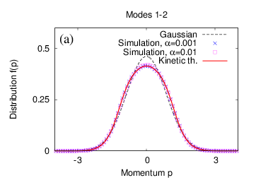
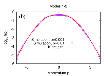
Figure 3: Stationary momentum distribution $f(p)$, on (a) linear, and (b) semi-log scales, for $\alpha=0.001$, and $0.01$ at kinetic temperature $T=0.75$. The plots correspond to modes $1$ and $2$ excited with amplitudes satisfying $c_{1}=c_{2}=C(0)/4$, where $C(0)=2T$. The data denoted by crosses and squares are results of $N$-body simulations of the stochastically-forced HMF model with $N=10000,\Delta t=0.01$ and $1000$ independent realizations of the dynamics, while the red continuous lines refer to the theoretical prediction from the kinetic theory. For comparison, the black broken line shows the Gaussian distribution with the same kinetic energy (stationary state of the stochastically-forced HMF model at $T=0.75$, $c_{0}=c_{1}=0,c_{2}=0.75,c_{k\geq 3}=0$).

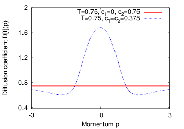
Figure 4: Diffusion coefficient $D[f](p)$ for the stationary momentum distribution $f(p)$ at kinetic temperature $T=0.75$, with $c_{0}=c_{k\geq 3}=0$, and either (i) $c_{1}=c_{2}=0.375$, or, (ii) $c_{1}=0,c_{2}=0.75$.

We now focus on how to obtain from the kinetic equation (32) predictions for the nonequilibrium stationary states of the system. According to Eq. (32), $1/\alpha$ is only a timescale; thus, at leading order in $\alpha$ and except for a time rescaling, the parameter $\alpha$ does not affect the time evolution of the system. This statement holds also beyond the leading order for what concerns the evolution of the kinetic energy; its evolution may be obtained directly from the equations of motion (3), as discussed in section 2, and can also be obtained from the kinetic equation (32), as detailed in C. For the evolution of other observables, there will be corrections at higher orders in $\alpha$.

As previously discussed, the dynamics of the system does not respect detailed balance if the forcing is not white in space. At the level of the kinetic equation, by inspecting the definition of the diffusion coefficient, Eq. (33), we see that the effect of correlations induced by the stochastic forces is modulated by the Fourier component $v_{k}$ of the interparticle potential. Then, taking the forcing spectral amplitudes $c_{k}$ different from zero if and only if $v_{k}=0$, the non-linear part of the diffusion coefficient vanishes. On the other hand, taking $c_{k}\neq 0$ for the modes for which $v_{k}\neq 0$ leads to a diffusion constant which has a non-vanishing non-linear part. To be concrete, let us discuss these two scenarios in the context of the stochastically-forced HMF model.

Since the Fourier transform of the HMF interparticle potential is, for $k\neq 0$, $v_{k}=-\left[\delta_{k,1}+\delta_{k,-1}\right]/2$, it follows that only the stochastic force mode with wave number $k=1$ contributes to the non-linear part of the diffusion coefficient; all the other stochastic force modes result in only a mean-field contribution through the term $C(0)$. Thus, for the case $c_{1}\neq 0$, the two relevant parameters that dictate the evolution of the stochastically-forced HMF model by the kinetic equation (32) with a non-linear diffusion coefficient are $C(0)$ and $c_{1}$. From Eq. (12), since $C(0)$ is related to the kinetic temperature $T$, we take $T$ and $c_{1}$ to be the two relevant parameters. From Eq. (11), we know that $2T$ equals the kinetic energy in the final stationary state. Also, Eq. (4) implies that $c_{1}\leq C(0)/2$.

If however $c_{1}=0$, then, at leading order in $\alpha$, the dynamics of the system is described by a linear Fokker-Planck equation; this equation is the same as the one which describes the HMF system when coupled to a Langevin thermostat, studied in [31, 30]. This means that for this particular choice of the parameters, the detailed balance is broken for the dynamics, but this feature cannot be seen in the kinetic theory, being an effect at a higher order in $\alpha$. In this case, the homogeneous stationary states of the kinetic equation have Gaussian momentum distribution $f(p)$. As has been studied thoroughly in the context of canonical equilibrium of the HMF model, these states are stable for kinetic energies greater than $1/4$, i.e., for $C(0)>1$.

Except for the special case of $c_{1}=0$, the stationary velocity distribution of the kinetic equation (32) is in general not Gaussian. This can be seen semi-analytically by observing that the Gaussian distribution function

$$f_{G}(p)=A\,\exp(-\beta p^{2})\,,\qquad A=\sqrt{\frac{\beta}{\pi}}\,,\qquad\beta=\frac{1}{2T},$$ (37)

with $\beta$ chosen such that the value of the kinetic energy is the one selected by $T$, solves the linear Fokker-Planck equation with the diffusion coefficient given by

$$D_{mf}=T.$$ (38)

To prove that the Gaussian distribution function is not a stationary solution of Eq. (32), we have to prove that the contribution to $\partial f/\partial t$ from the non-linear part of $D[f](p)$ in Eq. (33) does not vanish. This result can be proven with an asymptotic expansion [12] for large momenta of the integrals which appear in the diffusion coefficient. We report the straightforward computation in D. From the same analysis, one can deduce that, even though the distribution function is not Gaussian, its tails are Gaussian.

On the basis of the above discussions, we expect that for values of $T$ and $c_{1}$ such that $T>0.5$ and $c_{1}\ll 2T$, the stationary states will be close to homogeneous states with Gaussian momentum. In order to locate the actual stationary states of the kinetic equation, we have devised a simple numerical scheme, based on the observation that a linear Fokker-Planck equation whose diffusion coefficient $D(p)$ is strictly positive admits a unique stationary state

$$f_{ss}(p)=A\exp\left[-\int_{0}^{p}{\rm d}p^{\prime}\leavevmode\nobreak\ \frac{p^{\prime}}{D(p^{\prime})}\right].$$ (39)

For a given distribution $f_{n}(p)$, we compute the diffusion coefficient $D_{n}(p)$ through Eq. (33), and then $f_{n+1}$ using $D_{n}$ and Eq. (39). This procedure defines an iterative scheme. Whenever convergent, this scheme leads to a stationary state of Eq. (32). Each iteration involves integrations, so that we expect the method to be robust enough when starting not too far from an actual stationary state. However, we have no detailed mathematical analysis yet. Implementing this iterative scheme, we observed that the distribution $f_{\infty}$ to which the scheme converges is independent of the initial distribution $f_{0}$. Moreover, the convergence time is exponential in the number of steps $n$ whenever $T$ is not too close to loss of stability of $f_{\infty}$ with respect to the linear Vlasov dynamics; in practice, we are able to get reliable results for $T\gtrsim 0.65$.

In order to check the theoretical predictions discussed above, we performed numerical simulations of the stochastically forced HMF model. Figure 2 shows the evolution of the kinetic energy and $\langle p^{4}\rangle=(1/N)\sum_{i=1}^{N}p_{i}^{4}$, where they have been compared with our theoretical predictions. In the case of $\langle p^{4}\rangle$, we have compared the long-time asymptotic value with the kinetic theory prediction for the stationary state, computed numerically by using the iterative solution for the stationary distribution. The figure illustrates a very good agreement between the theory and simulations. For a more accurate check of the agreement, we have obtained the stationary momentum distribution from both $N$-body simulations and the numerical iterative scheme discussed above. A comparison between the two, shown in Fig. 3, both on linear and semi-log scales, shows a very good agreement between theory and simulations. In this figure, we also show the Gaussian distribution with the same kinetic energy, to illustrate the point that the stationary momentum distribution of the system is far from being Gaussian. The diffusion coefficient $D[f](p)$ is shown in figure 4.

In passing, let us remark that, with an iterative scheme analogous to the one described above, one could have also obtained the full time evolution $f(p,t)$ that obeys the kinetic equation (32). However, we will not address this point here.

We also note that while a linear Fokker-Planck equation with non-degenerate diffusion coefficient can be proven to converge to a unique stationary distribution [25], this is not true in general for non-linear Fokker-Planck equations like Eq. (32). We expect that if the dynamics is not too far from detailed balance, the kinetic equation will have a unique stationary state. Far from equilibrium, the kinetic equation could lead to very interesting dynamical phenomena, like bistability, limit cycle or more complex behaviors. The main issue is then the analysis of the evolution of the kinetic equation. Although some methods to study this type of equation exist [32], we have only the numerical iterative scheme described above to provide some preliminary answers. A more rigorous mathematical analysis is left for future studies.

5 Nonequilibrium phase transition and collapse

Until now, we have considered homogeneous stationary states of the dynamics (3), and have discussed a kinetic theory to analyze them. Although our theory can in principle be extended to include inhomogeneous stationary states, its actual implementation to get, e.g., the single-particle distribution, would require more involved computations than the one we encountered for homogeneous states. In order to get preliminary answers, we have performed extensive numerical simulations of the dynamics in the context of the stochastically-forced HMF model. Our specific interest is to know about how the magnetization behaves as the kinetic temperature is reduced from high values.

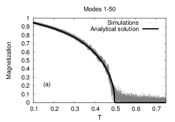
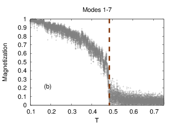
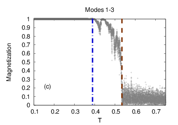
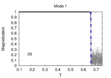
Figure 5: Numerical simulation results for magnetization in the stochastically-forced HMF model as a function of adiabatically-tuned kinetic temperature $T$; the different plots correspond to different number of modes excited in the spectrum with amplitudes satisfying $C(0)=c_{0}+2\sum_{k=1}^{N_{R}}c_{k}$, where $C(0)=2T$, the index $k=1,2,\ldots,N_{R}$ denotes the mode number, while $N_{R}$ is the total number of excited modes with $k\neq 0$. In all cases, the modes excited were chosen to have equal amplitudes, with $c_{0}=0,N=5000,\alpha=0.01,\Delta t=0.01$, while the tuning rate for $T$ is $10^{-5}$. It may be noted that forcing equally a large number of modes ($\sim 50$) reproduces the equilibrium magnetization profile as illustrated by the match with the analytical equilibrium solution in the panel (a). In panel (b), the first-order nonequilibrium phase transition is marked by the vertical dashed line. In panel (c), besides the first-order transition, we also show the dynamical transition to the collapsed state by the vertical dashed dotted line. In panel (d), the nonequilibrium phase transition and the dynamical transition almost coincide, and we just show the latter one by the vertical dashed dotted line.

In the case when the stochastic forcing respects detailed balance (i.e., when the noise spectrum is flat and all modes are excited), the stochastically-forced HMF model reduces to the Brownian mean-field (BMF) model studied previously [31]. Here, we know that the system settles into an equilibrium state in which it exhibits a second-order phase transition at the kinetic temperature $T=T_{c}=1/2$: on increasing $T$ from low values, the magnetization decreases continuously to zero at $T_{c}$ and remains zero at higher temperatures. In the following, we excite only a limited number of modes $N_{R}$, but the amplitudes of all excited modes are equal ($c_{k}$ equals $c$ for all $k\leq N_{R}$, and is zero otherwise, where the constant $c$ is related to the temperature). Figure 5(a) shows that with $N_{R}=50$, one reproduces very well the equilibrium profile of the magnetization as a function of temperature. On reducing the value of $N_{R}$, the system is driven more and more out of equilibrium. Indeed, Fig. 5(b) shows that with $N_{R}=7$, the magnetization profile changes; in particular, it develops a discontinuity around a temperature $T_{trans}\approx 0.49$, reminiscent of a first-order phase transition. The transition temperature is denoted by the vertical dashed line. With $N_{R}=3$, Fig. 5(c) shows that the discontinuity gets more pronounced, and $T_{trans}$ is now shifted to a higher value (denoted again by the vertical dashed line). A new feature appears in this plot, namely, at a temperature $T_{dyn}\approx 0.4$, the magnetization attains the maximal value of unity, which it retains for all lower temperatures. This value of unity corresponds to a state in which the particles are very close to one another on the circle, thus defining a “collapsed” state. We found that this state, as well as the transition to it, persist on changing the system size $N$.

Now, it is known that trajectories of ensembles of dissipative dynamical systems forced by the same realization of a stochastic noise converge to a single one [33, 34]. These attracting trajectories are referred to as the ones due to the so-called stochastic attractor. Although we did not perform a detailed characterization of the collapse in our model, we believe that the phenomenon is related to stochastic attractors.

Coming back to Fig. 5(c), we see that for temperatures $T_{dyn}<T<T_{trans}$, the magnetization shows strong fluctuations. Reducing the number of excited modes to a single one, namely, to the one that coincides with the Fourier mode of the HMF potential, it seems from Fig. 5(d) that only the dynamical transition to the collapsed state at a temperature $T_{dyn}\approx 0.66$ persists.

The hint that the nature of the phase transition at $T_{trans}$ is of first-order comes from the hysteresis plots of Fig. 6. To obtain these plots, one monitors the magnetization while tuning adiabatically the kinetic temperature across $T_{trans}$ from higher to lower values and back to complete a full cycle. As is evident from Fig. 6, the observed hysteresis is between the collapsed state and the zero-magnetization state. In principle, it should be possible to observe a hysteretical behavior between the magnetized and the zero-magnetization state. To achieve this in simulations involving adiabatic tuning of temperature, one should not allow the system to make the transition to the collapsed state, which requires conditions close to those that ensure detailed balance. However, a possible drawback of this method is that closeness to detailed balance might lead to narrow hysteresis loops. Moreover, the adiabatic tuning of temperature should not be very slow, as otherwise one observes bistability instead of the hysteresis. All these factors make the observation of hysteresis between the magnetized and the zero-magnetization state difficult to observe numerically; further explorations of this will be the subject of future investigations.

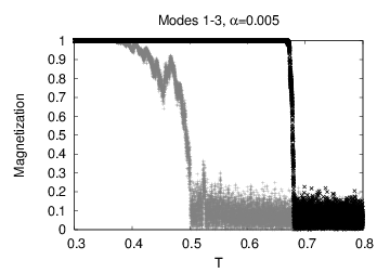
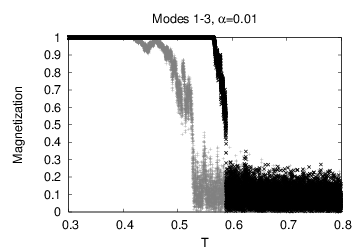
Figure 6: Numerical simulation results for magnetization in the stochastically-forced HMF model as a function of adiabatically-tuned kinetic temperature $T$ for two different values of $\alpha$. In each case, the modes $1-3$ are excited with amplitudes satisfying $c_{1}=c_{2}=c_{3}=C(0)/6$, where $C(0)=2T$. In all cases, $N=5000,\Delta t=0.01$, while the tuning rate for $T$ is $10^{-5}$. The grey points correspond to the case when the temperature is decreased from high values, while the black points correspond to the case when the temperature is increased from low values.

In order to explore further the region in Fig. 5(c) close to $T_{trans}$, and to ascertain the nature of the phase transition at $T_{trans}$, we fix the value of the temperature to be $T=0.53$, and monitor the magnetization as a function of time. The time series of the magnetization is shown in Fig. 7(a), in which one observes clear signatures of bistability, whereby the system switches back and forth between homogeneous ($m\approx 0$) and inhomogeneous ($m>0$) states. In addition, we show in Fig. 7(b) the distribution of the magnetization around the phase transition temperature: the distribution is bimodal with a peak around a zero value and another one around a positive value. When decreasing the temperature across the phase transition region, we clearly see that the peak heights of the distributions of the magnetization at the zero and non-zero values interchange. These two features, together with the hysteresis plots of Fig. 6, support the first-order nature of the transition around $T_{trans}$ which can be estimated from Fig. 7(b) to be $T_{trans}\approx 0.532$.

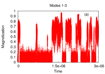
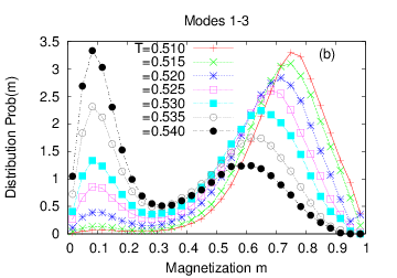
Figure 7: (a) Numerical simulation results for magnetization in the stochastically-forced HMF model as a function of time at kinetic temperature $T=0.53$, with $N=5000,\alpha=0.005,\Delta t=0.01$, and with modes $1-3$ excited, whose amplitudes satisfy $c_{1}=c_{2}=c_{3}=C(0)/6$, where $C(0)=2T$. The figure shows clear signatures of bistability in which the system during the course of evolution switches back and forth between spatially homogeneous ($m\sim O(0)$) and inhomogeneous ($m\sim O(1)$) states. (b) Distribution $Prob(m)$ of the magnetization $m$ as a function of $T$ at a fixed value of $\alpha=0.01$. The data are obtained from numerical simulation results similar to (a) for magnetization in the stochastically-forced HMF model, with $N=5000,\Delta t=0.01$, and with modes $1-3$ excited, whose amplitudes satisfy $c_{1}=c_{2}=c_{3}=C(0)/6$, where $C(0)=2T$.

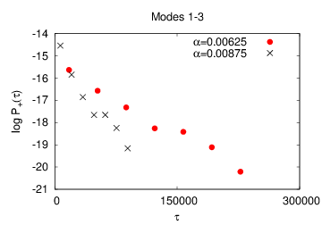
Figure 8: Distribution of the residence time $\tau$ in the inhomogeneous state, for two values of $\alpha$. The data are obtained from simulations with modes $1-3$ excited, whose amplitudes satisfy $c_{1}=c_{2}=c_{3}=C(0)/6$, where $C(0)=2T$. Here, the kinetic temperature $T=0.53$, while $\Delta t=10^{-2},N=5000$.

From Fig. 7, it is clear that the system has two well separated attractors, corresponding to the homogeneous and inhomogeneous states. A question of immediate interest is: How long does the system stay in one state before switching to the other? Let us define the residence time as the time the system stays in one state before it switches to the other. In the limit of low noise level $\alpha$, there is a clear separation between the natural dynamical time and the typical residence time, as is evident from Fig. 7(a). As a result, one may conjecture that two successive switching events are statistically independent of one another. In case such a conjecture holds for our model, the residence time statistics will be a Poisson process, characterized solely by the probability per unit time, $\lambda_{+}$, of switching from the inhomogeneous state to the homogeneous state, and the probability per unit time, $\lambda_{-}$, for the reverse switch. The distribution of residence time $\tau$ in each phase is then exponential:

$$P_{\pm}(\tau)=\frac{1}{\lambda_{\pm}}\exp(-\lambda_{\pm}\tau),$$ (40)

so that the average residence times in the two states are $\tau^{res}_{\pm}=\frac{1}{\lambda_{\pm}}$. Such an exponential form of the residence time distribution is verified from our simulation data displayed in Fig. 8. Note that generating such a plot requires running simulations of the dynamics for long enough times so that the magnetization switches back and forth between the two states a sufficient number of times, and one has good statistics for the residence times. For low values of $\alpha$, such as those used in Fig. 8, this was often not feasible due to very long simulation times. This results in bad statistics, and hence, the form of the plot displayed in Fig. 8, which, though good, may be improved upon by running longer simulations. We conclude that our conjecture of two successive jumps being independent holds for our model, and that the average residence time fully characterizes the switching process for small enough $\alpha$.

We now discuss how the residence times depend on the system parameters, in particular, on $\alpha$. For an equilibrium system, the type of switching process described above is an activation process with a residence time described by the Arrhenius law. A simple model of such an activation process is the Langevin dynamics of a Hamiltonian system in a potential $\mathcal{V}$. The noise level is then related to the temperature, and the Arrhenius law takes the form [35, 22, 36, 37]

$$\tau^{res}_{+}\propto\exp(\Delta\mathcal{V}_{+-}/\alpha),$$ (41)

$$\tau^{res}_{-}\propto\exp(\Delta\mathcal{V}_{-+}/\alpha).$$ (42)

Here, $\Delta\mathcal{V}_{+-}$ and $\Delta\mathcal{V}_{-+}$ are respectively the potential energy barrier as observed from the inhomogeneous and the homogeneous state. In a non-equilibrium context such as ours, there is no obvious equivalent of a potential, but the law given by Eqs. (41) and (42) is expected to hold on a fairly general basis, in the limit of small noise. This may be established from the instanton theory, or, from the Freidlin-Wentzell theory, which allows to compute $\mathcal{V}$ explicitly for a given model [38, 39]. Our system does not fulfill the hypothesis of Freidlin-Wentzell theory, nevertheless, it is interesting to check if the law given by Eqs. (41) and (42) holds. Our simulation data shown in Fig. 9 show that the dependence of $\tau^{res}_{\pm}$ on $\alpha$, as in Eqs. (41) and (42), holds also for our model, thereby suggesting that in the limit of low noise, the system behaves as one with transitions activated by a weak noise.

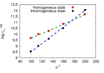
Figure 9: The plot shows as a function of $1/\alpha$ the $\log$ of the mean residence time $\tau^{res}_{+,-}$ in the two bistable states, namely, the inhomogeneous ($m>0$) state and the homogeneous state ($m\approx 0$). The plot is based on data obtained from simulations with modes $1-3$ excited, whose amplitudes satisfy $c_{1}=c_{2}=c_{3}=C(0)/6$, where $C(0)=2T$. Here, the kinetic temperature $T=0.53$, while $\Delta t=10^{-2},N=5000$. The straight line fits imply that $\tau^{res}_{+,-}\sim\exp(1/\alpha)$, in accordance with Eqs. (41) and (42). That the slopes of the two straight lines in the plot are different could be due to the fact that the height of the barrier is different when observed from the inhomogeneous and the homogeneous state.

We conclude this section by describing briefly the algorithm to find $P_{\pm}(\tau^{\pm})$ to produce Fig. 8, and $\tau^{res}_{\pm}$ to produce Fig. 9. To this end, one has to identify from the time series data of the magnetization (see Fig. 7(a) for an example) the switching time instants between the two states. In the limit of very small $\alpha$, the distinction between two states should be obvious. However, we could not reach such a limit in our numerical simulations because the simulation time grows exponentially with $1/\alpha$ (see Fig. 9). For intermediate values of $\alpha$, it is then a challenge to define precisely the two states. Indeed, as may be seen in Fig. 7(a), the data show strong fluctuations and hence, one needs to filter out “spurious” switching events and retain only the genuine ones. This may be done efficiently as we now discuss.

We first obtain from the data a rough estimate of the mean of the magnetization when the system is in the two states, the homogeneous and the inhomogeneous one. Let us denote by $m_{>}$ and $m_{<}$ these estimates when the system is in the inhomogeneous and the homogeneous state, respectively. Let us define a “threshold” value of the magnetization $m_{th}$ as the average of $m_{>}$ and $m_{<}$; magnetization crossing this threshold to switch from one state to another however is not a precise enough criterion to define a switching event, as is obvious from Fig. 7. We thus resort to our algorithm which we now illustrate for the case when the system is in the homogeneous state; when the system is in the inhomogeneous state, the algorithm may be defined in a manner similar to the one below. In our algorithm, we identify a switching event as the one for which the following two conditions are satisfied, namely, (i) that the magnetization crosses the threshold to switch from the homogeneous to the inhomogeneous state, (ii) the magnetization after the switching reaches the value $m_{>}$ before reaching the value $m_{<}$. When a switching event occurs, the switching time is defined as the time at which the magnetization crossed the threshold. This algorithm allows us to precisely define the switching times, from which we compute the switching time statistics $P_{\pm}(\tau_{\pm})$, and hence, the mean residence time $\tau^{res}_{\pm}$.

6 Conclusions

In this work, we considered long-range interacting systems driven by external stochastic fields, thereby leading to generic nonequilibrium stationary states. To study spatially homogeneous stationary states, we developed a kinetic theory approach by generalizing the known results for isolated long-range systems. Our theoretical approach is quite general, being applicable to any long-range inter-particle potential, space dimensions and boundary conditions. Our extensive numerical simulations on a paradigmatic model of long-range interacting systems demonstrated a very good agreement with the theory. Besides, our simulations for this representative case illustrated very interesting bistable behavior between homogeneous and inhomogeneous states, with a mean residence time that diverges as an exponential in the inverse of the strength of the external stochastic forces in the limit of low values of such forces.

Let us note that another route to deriving the kinetic theory studied in this paper is to adopt an approach similar to the one due to Klimontovich for isolated systems, by writing down the time evolution equation for the noise-averaged empirical measure $\rho(p,q,t)=(1/N)\sum_{i=1}^{N}\langle\delta(q_{i}(t)-q)\delta(p_{i}(t)-p)\rangle$. In the resulting equation, the noise appears as a multiplicative term, which can be treated perturbatively, leading to the kinetic equation (32).

This work leaves open some interesting issues, e.g., for technical simplicity, we assumed a homogeneous stationary state for the development of the kinetic theory. It would be of interest to generalize the theory to inhomogeneous states; in this regard, the method due to Heyvaerts reported recently may come of help [40]. Another issue is to study the dynamics of the kinetic equation (32), both analytically and numerically, which may unveil very interesting behaviors, such as limit cycles. One may also hope to develop a kinetic theory similar to the one analyzed here for related systems, for example, the point vortex model and the Euler equations in two-dimensional turbulence [5].

7 Acknowledgments

C. N. acknowledges the EGIDE scholarship funded by Ministère des Affaires Étrangères. S. G. and S. R. acknowledge the contract LORIS (ANR-10-CEXC-010-01). F. B. acknowledges the ANR program STATOCEAN (ANR-09-SYSC-014). Numerical simulations were done at PSMN, ENS-Lyon. S. G. is grateful to the Korea Institute for Advanced Study (KIAS), Seoul for the kind hospitality during the time part of this work was being done and written up.

Appendix A Condition of detailed balance for the dynamics (3)

We prove here that the dynamics defined by the equations of motion (3) satisfies detailed balance if and only if $c_{k}=c$ for all $k$, that is, if the stochastic forcing has a white spectrum in space.

We start from the $N$-particle Fokker-Planck equation (14) associated with the equations of motion (3). It will be useful to rewrite it in the following way:

$$\frac{\partial f_{N}(\mathbb{x})}{\partial t}=-\sum_{i=1}^{2N}\frac{\partial}{\partial x_{i}}[A_{i}(\mathbb{x})f_{N}(\mathbb{x})]+\frac{1}{2}\sum_{i,j=1}^{2N}\frac{\partial^{2}}{\partial x_{i}\partial x_{j}}[B_{i,j}(\mathbb{x})f_{N}(\mathbb{x})]\,,$$ (43)

where $x_{i}=q_{i}$ for $i=1,...,N$, $x_{i}=p_{i-N}$ for $i=(N+1),...,2N$, and we use the notation $\mathbb{x}=\{x_{i}\}$. The drift vector $A_{i}(\mathbb{x})$ is a function of the $x_{i}$’s, and is given by

$$A_{i}(\mathbb{x}) =p_{i}\qquad{\rm for}\qquad i=1,...,N,$$ (44)

$$A_{i}(\mathbb{x}) =-\alpha p_{i-N}-\frac{1}{N}\sum_{j=1}^{N}\frac{\partial v(q_{i-N}-q_{j})}{\partial q_{i-N}}\qquad{\rm for}\qquad i=(N+1),...,2N.$$ (45)

Similarly, the expression for the (symmetric) diffusion matrix $B_{i,j}$ is:

$$B_{i,j}(\mathbb{x})=\alpha C(|q_{i-N}-q_{j-N}|)\qquad{\rm for}\qquad i>N\,\wedge\,j>N,$$ (46)

and $B_{i,j}(\mathbb{x})=0$ otherwise. We moreover introduce the constants $\varepsilon_{i}=\pm 1$, which denote the parity with respect to time inversion of the variables $x_{i}$, and the notation $\varepsilon\mathbb{x}=\{\varepsilon_{i}x_{i}\}$.

It can be shown (see [22], Sect. 5.3.5, or [25], Sect. 6.4) that the dynamics described by a Fokker-Planck equation of the form (43) satisfies detailed balance if and only if the following two conditions are satisfied ($i=1,...,2N$):

$$\varepsilon_{i}\varepsilon_{j}B_{i,j}(\mathbb{\varepsilon x})=B_{i,j}(\mathbb{x}),$$ (47)

and

$$\varepsilon_{i}A_{i}(\varepsilon\mathbb{x})f^{s}_{N}(\mathbb{x})=-A_{i}(\mathbb{x})f^{s}_{N}(\mathbb{x})+\sum_{j=1}^{2N}\frac{\partial}{\partial x_{j}}B_{i,j}(\mathbb{x})f^{s}_{N}(\mathbb{x}),$$ (48)

where $f^{s}_{N}(\mathbb{x})$ is the stationary solution of (43).

In our case, in which the drift and the diffusion terms are given by Eqs. (44) and (46), respectively, the condition (47) is trivially satisfied. Our proof goes as follows: we solve formally Eq. (48), and show that $f^{s}_{N}(\mathbb{x})$ is a stationary solution of Eq. (43) if and only if the non-vanishing part of $B_{i,j}$ is proportional to the identity matrix. Then, it is simple to show that this implies that the spectrum of the forcing has to be white in space.

Equation (48) for $i=1,...,N$ is also trivially satisfied. On the other hand, for what concerns $i=(N+1),...,2N$, we have

$$2p_{k}f^{s}_{N}(\mathbb{x})=-\sum_{j=1}^{N}C(|q_{k}-q_{j}|)\frac{\partial f^{s}_{N}(\mathbb{x})}{\partial p_{j}},$$ (49)

where $k=i-N$. We introduce the $N\times N$ matrix $\mathcal{C}$ whose components are given by $\mathcal{C}_{k,j}(\mathbb{x})=C(|q_{k}-q_{j}|)$, and observe that, for generic values of the $q_{i}$’s, $\mathcal{C}$ admits an inverse $\mathcal{C}^{-1}$. Integrating Eq. (49), we thus have

$$f^{s}_{N}(\mathbb{x})=d(q_{1},...,q_{N})\exp\left[-\sum_{k,j=1}^{N}p_{k}\left(\mathcal{C}^{-1}\right)_{k,j}p_{j}\right],$$ (50)

where $d(q_{1},...,q_{N})$ is an undetermined function. Inserting Eq. (50) into the Fokker-Planck equation (43), imposing that it is a stationary solution, and with some calculations, we get

$$\sum_{i=1}^{N}\left[-\frac{\partial f^{s}_{N}}{\partial q_{i}}\frac{\partial H}{\partial p_{i}}+\frac{\partial H}{\partial q_{i}}\frac{\partial f^{s}_{N}}{\partial p_{i}}\right]=0\,.$$ (51)

Then, $f^{s}_{N}$ is a function of the Hamiltonian $H$, that is $f^{s}_{N}(\mathbb{x})=\psi(H(\mathbb{x}))$ for some function $\psi$. On the other hand, because $f^{s}_{N}$ is given by the formula in Eq. (50), we can also deduce that $\psi$ is an exponential, and thus, that $f^{s}_{N}$ is Gaussian in the velocities. We conclude that $\mathcal{C}^{-1}$ (and hence, $\mathcal{C}$) has to be independent of the $q_{i}$’s and proportional to the identity. Finally, from the form of $C(|q_{i}-q_{j}|)$ in Eq. (4), we see that this condition on $\mathcal{C}$ is satisfied if and only if the spectrum of the forcing is white in space.

Appendix B Closure of the BBGKY hierarchy (3.1)

We analyze here in detail the closure of the BBGKY hierarchy discussed in the text, in particular, the reasons for which the connected part of the two-particle correlation is of order $\alpha$, while higher correlations are negligible at leading order in $\alpha$, so that this closure is self-consistent.

In the following, we expand the functions $f_{2}$ and $f_{3}$ as

$$f_{2}(z_{1},z_{2},t)=f(z_{1},t)f(z_{2},t)+\tilde{g}(z_{1},z_{2},t),$$ (52)

and

$$f_{3}(z_{1},z_{2},z_{3},t) = f(z_{1},t)f(z_{2},t)f(z_{3},t)+f(z_{1},t)\tilde{g}(z_{2},z_{3},t)$$ (53)

$$+f(z_{2},t)\tilde{g}(z_{1},z_{3},t)+f(z_{3},t)\tilde{g}(z_{1},z_{2},t)+h(z_{1},z_{2},z_{3},t),$$

and similarly, for other $f_{s}$’s for $s\geq 4$.

Now, let us write explicitly the first two equations of the BBGKY hierarchy (3.1). The first one, obtained from Eqs. (3.1) and (52), is

$$\frac{\partial f}{\partial t}+p\frac{\partial f}{\partial q}-\frac{\partial f}{\partial p}\frac{\partial\Phi[f]}{\partial q}-\alpha\frac{\partial}{\partial p}[pf]-\frac{\alpha}{2}C(0)\frac{\partial^{2}f}{\partial p^{2}}=\frac{\partial}{\partial p}\int{\rm d}q_{1}{\rm d}p_{1}\,v^{\prime}(q-q_{1})\tilde{g}(z,z_{1},t),$$ (54)

where

$$\Phi[f](q)=\int{\rm d}q_{1}{\rm d}p_{1}\,v(q-q_{1})f(q_{1},p_{1},t)$$ (55)

is the mean-field potential. For the second equation of the hierarchy, we use Eqs. (53) and (54) to get

$$\frac{\partial\tilde{g}(z_{1},z_{2},t)}{\partial t} = \Big{[}-p_{1}\frac{\partial\tilde{g}}{\partial q_{1}}+\frac{\partial\tilde{g}}{\partial p_{1}}\frac{\partial\Phi[f]}{\partial q_{1}}+\frac{f(z_{2})}{N}\frac{\partial v(q_{1}-q_{2})}{\partial q_{1}}\frac{\partial f}{\partial p_{1}}+\frac{1}{N}\frac{\partial v(q_{1}-q_{2})}{\partial q_{1}}\frac{\partial\tilde{g}}{\partial p_{1}}$$ (56)

$$+\frac{\partial f}{\partial p_{1}}\int{\rm d}z_{3}\frac{\partial v(q_{1}-q_{3})}{\partial q_{1}}\tilde{g}(z_{2},z_{3})+\frac{\partial}{\partial p_{1}}[\alpha p_{1}\tilde{g}]+\frac{\alpha}{2}C(|q_{1}-q_{2}|)\frac{\partial f}{\partial p_{1}}\frac{\partial f}{\partial p_{2}}$$

$$+\frac{\alpha}{2}C(0)\frac{\partial^{2}\tilde{g}}{\partial p_{1}^{2}}+\frac{\alpha}{2}C(|q_{1}-q_{2}|)\frac{\partial^{2}\tilde{g}}{\partial p_{1}\partial p_{2}}+\int{\rm d}z_{3}\,\frac{\partial v(q_{1}-q_{3})}{\partial q_{1}}\frac{\partial h}{\partial p_{1}}\Big{]}$$

$$+\{1\leftrightarrow 2\},$$

where the symbol $\{1\leftrightarrow 2\}$ stands for an expression obtained from the bracketed one on the right hand side by exchanging the subscripts $1$ and $2$.

Let us analyze the order of magnitude of various terms in Eq. (56). First of all, we have $f\sim 1$, as it is normalized to unity. However, we do not know a priori the order of magnitude of $\tilde{g}$ and $h$. Thus, the order of magnitude of all but the terms $\frac{f(z_{2})}{N}\frac{\partial v(q_{1}-q_{2})}{\partial q_{1}}\frac{\partial f}{\partial p_{1}}$ and $\frac{\alpha}{2}C(|q_{1}-q_{2}|)\frac{\partial f}{\partial p_{1}}\frac{\partial f}{\partial p_{2}}$ is unknown. In the continuum limit $N\alpha\gg 1$, we have

$$\frac{f(z_{2})}{N}\frac{\partial v(q_{1}-q_{2})}{\partial q_{1}}\frac{\partial f}{\partial p_{1}}\sim\frac{1}{N}\ll\alpha\sim\frac{\alpha}{2}C(|q_{1}-q_{2}|)\frac{\partial f}{\partial p_{1}}\frac{\partial f}{\partial p_{2}},$$ (57)

so that it is natural to guess that $\tilde{g}\sim\alpha$. Let us also observe that in the limit $N\alpha\ll 1$, we have

$$\frac{f(z_{2})}{N}\frac{\partial v(q_{1}-q_{2})}{\partial q_{1}}\frac{\partial f}{\partial p_{1}}\sim\frac{1}{N}\gg\alpha\sim\frac{\alpha}{2}C(|q_{1}-q_{2}|)\frac{\partial f}{\partial p_{1}}\frac{\partial f}{\partial p_{2}},$$ (58)

so that we obtain $\tilde{g}\sim 1/N$. In the limit $N\alpha\ll 1$, the kinetic theory leads to the Lenard-Balescu equation.

Once we have established that $\tilde{g}\sim\alpha$, one can write down the equation of the hierarchy for $h$ and, with similar reasoning as above, one then finds that $h$ is at least of order $\alpha/N\ll\alpha$ (or, $\alpha^{2}$ depending on whether $\alpha/N\ll\alpha^{2}$ or the reverse), so that the term $\int{\rm d}z_{3}\,\frac{\partial v(q_{1}-q_{3})}{\partial q_{1}}\frac{\partial h}{\partial p_{1}}$ is negligible in Eq. (56), as may be straightforwardly checked. The iterative procedure can be repeated at all orders of the hierarchy. Discarding three-particle and higher-order correlations is thus a self-consistent procedure. Moreover, note that in Eq. (56), some of the terms are of higher orders ($\alpha^{2}$, $\alpha/N$,…) with respect to $\alpha$, and thus, can be discarded. The final form of the second equation of the BBGKY hierarchy is thus

$$\frac{\partial\tilde{g}(z_{1},z_{2})}{\partial t} = \Big{[}-p_{1}\frac{\partial\tilde{g}}{\partial q_{1}}+\frac{\partial\tilde{g}}{\partial p_{1}}\frac{\partial\Phi[f]}{\partial q_{1}}+\frac{\partial f}{\partial p_{1}}\int{\rm d}z_{3}v^{\prime}(q_{1}-q_{3})\tilde{g}(z_{2},z_{3})$$ (59)

$$+\frac{\alpha}{2}C(|q_{1}-q_{2}|)\frac{\partial f}{\partial p_{1}}\frac{\partial f}{\partial p_{2}}\Big{]}+\{1\leftrightarrow 2\}.$$

Note that $\tilde{g}\sim\alpha$ implies, see Eq. (54), that the mean-field effect of the stochastic forces gives a contribution at the same order to the two-particle correlation induced by them.

Appendix C Evolution of the kinetic energy for the dynamics (3)

We derive here the evolution of the kinetic energy as obtained from the kinetic equation (32). Let us recall that the average kinetic energy density at time $t$ in the continuous limit can be written as

$$\langle k(t)\rangle=\frac{1}{2}\int dp\,p^{2}\,f(p,t).$$ (60)

The starting point to obtain its time evolution is to multiply the kinetic equation (32) by $\frac{1}{2}p^{2}$, and then, to integrate over $p$. Neglecting for the moment the non-linear part of the diffusion coefficient, and integrating by parts, we get

$$\left\langle\frac{\partial k(t)}{\partial t}\right\rangle\,+\,2\alpha\,\langle k(t)\rangle\,-\,\frac{\alpha}{2}C(0)\,=0,$$ (61)

which gives

$$\langle k(t)\rangle\,=\,\left(\langle k(0)\rangle-\frac{C(0)}{4}\right)\,e^{-2\alpha t}\,+\,\frac{C(0)}{4}.$$ (62)

The kinetic energy density in the stationary state is thus $\left\langle\kappa\right\rangle_{ss}=C(0)/4$.

We now have to prove that the non-linear part of the diffusion coefficient (33) does not contribute to the time evolution of the kinetic energy. Such a result is expected and is usually valid for collisional terms (i.e., those terms in the kinetic equations which are given by two-particle correlation), for example, in the Boltzmann equation or in the Lenard-Balescu equation [28]. The contribution to $k(t)$ from the non-linear part of the diffusion coefficient is a sum of terms proportional to

$$T = \frac{1}{2}\int dp\,p^{2}\,$$

$$\times\frac{\partial}{\partial p}\,\left\{f^{\prime}(p,t)\left[\frac{1}{|\varepsilon(k,kp)|^{2}}\,\int^{*}dp_{1}\,\frac{f^{\prime}(p_{1},t)}{p_{1}-p}\,+\,\int^{*}dp_{1}\,\frac{f^{\prime}(p_{1},t)}{p_{1}-p}\frac{1}{|\varepsilon(k,kp_{1})|^{2}}\right]\right\};$$

we will show that each of such terms vanishes independently. Indeed, integrating the last expression over $p$ by parts, we get that

$$T=-\int dp\int^{*}dp_{1}\,p\,f^{\prime}(p,t)\left[\frac{f^{\prime}(p_{1},t)}{p_{1}-p}\,\frac{1}{|\varepsilon(k,kp)|^{2}}+\frac{f^{\prime}(p_{1},t)}{p_{1}-p}\,\frac{1}{|\varepsilon(k,kp_{1})|^{2}}\right].$$ (64)

Exchanging now the variables $p_{1}$ and $p$ and the order of integration, we get that the above equation may be rewritten as

$$T=\int dp\int^{*}dp_{1}\,p_{1}\,f^{\prime}(p_{1},t)\left[\frac{f^{\prime}(p,t)}{p_{1}-p}\,\frac{1}{|\varepsilon(k,kp_{1})|^{2}}+\frac{f^{\prime}(p,t)}{p_{1}-p}\,\frac{1}{|\varepsilon(k,kp)|^{2}}\right]\,.$$ (65)

Summing up the last two equations, we therefore have

$$T=\frac{1}{2}\int dp\,\int dp_{1}\,f^{\prime}(p_{1},t)\,f^{\prime}(p,t)\left[\frac{1}{|\varepsilon(k,kp_{1})|^{2}}+\frac{1}{|\varepsilon(k,kp)|^{2}}\right],$$ (66)

which vanishes on integrating by parts both with respect to $p_{1}$ and $p$.

Appendix D Proof that Eq. (32) admits non-Gaussian stationary distribution with Gaussian tails

We prove here that for a general forcing spectra, the Gaussian distribution function in Eq. (37) is not a stationary solution of the kinetic equation (32), and that the tails of any stationary state are Gaussian. For the first point, we have to prove that the contribution to $\partial f/\partial t$ from the non-linear part of $D[f](p)$ in Eq. (33) is not vanishing. This result can be proven with an asymptotic expansion [12] for large momenta of the integrals which appear in the diffusion coefficient. Given any function $g(p)$, we approximate integrals of the form

$$\int^{*}dp_{1}\frac{g(p_{1})}{p_{1}-p}$$ (67)

by expanding $\frac{1}{p_{1}-p}$ in Taylor series. We get, for example,

$$\int^{*}{\rm d}p_{1}\,\frac{f^{\prime}_{G}(p_{1})}{p_{1}-p}\,\simeq\,\frac{2}{\sqrt{\pi}}\beta^{3/2}\int_{-\infty}^{\infty}e^{-\beta p_{1}^{2}}\left[\frac{p_{1}}{p}+\left(\frac{p_{1}}{p}\right)^{2}+\left(\frac{p_{1}}{p}\right)^{3}+...\right]\,\simeq\,\frac{1}{p^{2}},$$ (68)

where, in the last equality, we have taken into account the fact that the Gaussian distribution being even, the terms containing $\left(\frac{p_{1}}{p}\right)^{k}$ with $k$ odd do not contribute. In a similar way, we have

$$|\varepsilon(k,kp)|^{2}\,\simeq\,1-\frac{4\pi v(k)}{p^{2}},$$ (69)

and

$$\int^{*}dp_{1}\,\left[\frac{f^{\prime}_{G}(p_{1})}{p_{1}-p}\frac{1}{|\varepsilon(k,kp_{1})|^{2}}\right]\,\simeq\,\frac{2\beta^{3/2}}{\sqrt{\pi}\,p^{2}}\,\int dp_{1}\,\frac{p_{1}^{2}\,e^{-\beta p_{1}^{2}}}{|\varepsilon(k,kp_{1})|^{2}},$$ (70)

where we have used the fact that $|\varepsilon(k,kp)|^{2}$ is an even function of $p$. With these results, we can evaluate the non-linear part of the kinetic equation: for large $p_{1}$, the non-linear contribution to $\partial f/\partial t$ is

$$2\pi\alpha\sum_{k=1}^{\infty}\,v_{k}\,c_{k}\left[1+\frac{2\beta^{3/2}}{\sqrt{\pi}}\,\int\,dp\,\frac{p^{2}e^{-p^{2}}}{|\varepsilon(k,kp)|^{2}}\right]\left[\frac{4\beta^{5/2}}{\sqrt{\pi}}\,e^{-\beta p_{1}^{2}}\right].$$ (71)

It can be shown that such a term is a non-vanishing function of $p_{1}$. This completes the proof: for a generic forcing spectra, the stationary state, when exists, is not Gaussian.

Using the same asymptotic expansion as before, it can be checked that the diffusion coefficient $D[f](p)$ converges to $C(0)/2$ for any distribution $f$. From this observation and Eq. (39), it follows that any stationary solution of the kinetic equation (32) has Gaussian tails.

References

References

- [1] Campa A, Dauxois T and Ruffo S, Statistical mechanics and dynamics of solvable models with long-range interactions, 2009 Phys. Rep. 480 57
- [2] Bouchet F, Gupta S and Mukamel D, Thermodynamics and dynamics of systems with long-range interactions, 2010 Physica A 389 4389
- [3] Chavanis P H, Phase transitions in self-gravitating systems, 2006 Int. J. Mod. Phys. B 20 3113
- [4] J. Stat. Mech. Topical Issue: Long-Range Interacting Systems
- [5] Bouchet F and Venaille A, Statistical mechanics of two-dimensional and geophysical flows, 2012 Phys. Rep. 515 227.
- [6] Weinberg M D, Noise driven evolution in stellar systems I. Theory, 2001 Mon. Not. R. Astron. Soc. 328 311
- [7] Liewer P C, Measurements of microturbulence in tokamaks and comparisons with theories of turbulence and anomalous transport, 1985 Nucl. Fusion 25 543
- [8] Dhar A, Heat transport in low-dimensional systems, 2008 Adv. Phys. 57 457
- [9] Derrida B, Non-equilibrium steady states: Fluctuations and large deviations of the density and of the current, 2007 J. Stat. Mech. P07023
- [10] Jarzynski C, Nonequilibrium work relations: Foundations and applications, 2008 Eur. Phys. J. B 64 331
- [11] Nicholson D R, Introduction to plasma physics, 1992 (Krieger, Malabar, Florida)
- [12] Lifshitz E M and Pitaevski L P, Physical kinetics, 2002 (Butterworth-Heinemann, London)
- [13] Bouchet F and Simonnet E, Random changes of flow topology in two-dimensional and geophysical turbulence, 2009 Phys. Rev. Lett. 102 94504
- [14] Briggs R J, Daugherty J D and Levy R H, Role of Landau damping in crossed-field electron beams and inviscid shear flow, 1970 Phys. Fluids 13 421
- [15] Dikii L A, The stability of plane-parallel flows of an ideal fluid, 1960 Dokl. Akad. Nauk SSSR 135 1068, Translated in Sov. Phys. Doklady 5, 1179
- [16] Nardini C, Gupta S, Ruffo S, Dauxois T and Bouchet F, Kinetic theory for non-equilibrium stationary states in long-range interacting systems, 2012 J. Stat. Mech. L01002
- [17] Chavanis P H, Kinetic theory of spatially homogeneous systems with long-range interactions: I. General results, 2012 Eur. Phys. J PLUS 127 19
- [18] Heggie D and Hut P, The gravitational million-body problem, 2003 (Cambridge University Press, Cambridge, UK)
- [19] Kac M, Uhlenbeck G E and Hemmer P C, On the van der Waals theory of the vapor-liquid equilibrium I. Discussion of a one-dimensional Model, 1963 J. Math. Phys. 4 216
- [20] Papoulis A, Probability, random variables and stochastic processes, 1965 (Tokyo: McGraw-Hill Kogakusha)
- [21] Rey-Bellet L, Ergodic properties of Markov processes, in Open Quantum systems II. The Markovian approach, Lecture notes in Mathematics 1881, 2006 (Springer, Berlin)
- [22] Gardiner C W, Handbook of stochastic methods for physics, chemistry and the natural sciences, 1983 (Springer-Verlag, Berlin)
- [23] Antoni M and Ruffo S, Clustering and relaxation in Hamiltonian long-range dynamics, 1995 Phys. Rev. E 52 2361
- [24] Yamaguchi Y Y, Barré J, Bouchet F, Dauxois T and Ruffo S, Stability criteria of the Vlasov equation and quasi-stationary states of the HMF model, 2004 Physica A 337 36
- [25] Risken H, The Fokker-Planck equation: Methods of solutions and applications, 1989 (Springer-Verlag, Berlin)
- [26] Huang K, Statistical mechanics, 1987 (Wiley, New York)
- [27] Nardini C and Bouchet F, 2013 (in preparation)
- [28] Balescu R, Statistical Dynamics: Matter Out of Equilibrium, 1987 (Imperial College Press, London)
- [29] McLachlan R I and Atela P, 1992 Nonlinearity 5 541
- [30] Baldovin F and Orlandini E, Nosé-Hoover and Langevin thermostats do not reproduce the nonequilibrium behavior of long-range Hamiltonians, 2007 Int. J. Mod. Phys. B 21 4000
- [31] Chavanis P H, Baldovin F and Orlandini E, Noise-induced dynamical phase transitions in long-range systems, 2011 Phys. Rev. E 83 040101(R)
- [32] Frank T D, Nonlinear Fokker-Planck Equations: Fundamentals and Applications, 2005 (Springer, Berlin)
- [33] Arnold L, Random dynamical systems, 2003 (Springer-Verlag, Berlin)
- [34] Maritan A and Banavar J R, Chaos, noise, and synchronization, 1994 Phys. Rev. Lett. 72 1451; Pikovsky A S, Comment on “Chaos, Noise, and Synchronization” 1994 Phys. Rev. Lett. 73 2931; Maritan A and Banavar J R, Maritan and Banavar Reply 1994 Phys. Rev. Lett. 73 2932
- [35] Kramers H A, Brownian motion in a field of force and the diffusion model of chemical kinetics, 1940 Physica 7 284
- [36] van Kampen N G, Stochastic processes in physics and chemistry, 1992 (North Holland, Amsterdam)
- [37] Hänggi P, Talkner P and Borkovec M, Reaction Rate Theory: Fifty Years After Kramers 1990 Rev. Mod. Phys. 62 251
- [38] Freidlin M I and Wentzell A D Random perturbations of dynamical systems, 1998 (Springer, Berlin)
- [39] Touchette H, The large deviation approach to statistical mechanics, 2009 Phys. Rep. 478 1
- [40] Heyvaerts J, A Balescu-Lenard-type kinetic equation for the collisional evolution of stable self-gravitating systems, 2010 Mon. Not. R. Astron. Soc. 407 355