Inference algorithms for pattern-based CRFs on sequence data
Rustem Takhanov Vladimir Kolmogorov
takhanov@mail.ruvnk@ist.ac.at Nazarbayev University, Kazakhstan
Institute of Science and Technology Austria
Abstract
We consider Conditional Random Fields (CRFs) with pattern-based potentials
defined on a chain. In this model the energy of a string (labeling)
is the sum of terms over intervals where each term is non-zero only if the substring
equals a prespecified pattern . Such CRFs can be naturally applied to many sequence tagging problems.
We present efficient algorithms for the three standard inference tasks in a CRF, namely
computing (i) the partition function, (ii) marginals, and (iii) computing the MAP.
Their complexities are respectively
, and
where is the combined length of input patterns, is the maximum length of a pattern,
and is the input alphabet.
This improves on the previous algorithms of [Ye et al. NIPS 2009] whose complexities are respectively ,
and ,
where is the number of input patterns. In addition, we give an efficient algorithm for sampling,
and revisit the case of MAP with non-positive weights.
††A preliminary version of this paper appeared in
Proceedings of the 30th International Conference on Machine Learning (ICML), 2013 [8]. This work was partially supported by the European Research Council under the European Unions Seventh Framework Programme (FP7/2007-2013)/ERC grant agreement no 616160.
This paper addresses the sequence labeling (or the sequence tagging) problem: given an observation
(which is usually a sequence of values), infer labeling
where each variable takes values in some finite domain .
Such problem appears in many domains such as text and speech analysis, signal analysis, and bioinformatics.
One of the most successful approaches for tackling the problem is the Hidden Markov Model (HMM).
The th order HMM is given by the probability distribution
with the energy function
(1)
where and is the substring of from to .
A popular generalization is the Conditional Random Field model [3] that allows all terms to depend
on the full observation :
(2)
We study a particular variant of this model called a pattern-based CRF.
It is defined via
(3)
where is a fixed set of non-empty words, is the length of word and is the Iverson bracket.
If we take then (3)
becomes equivalent to (2); thus we do not loose generality (but gain more flexibility).
Intuitively, pattern-based CRFs allow to model long-range interactions for selected subsequences of labels.
This could be useful for a variety of applications:
in part-of-speech tagging patterns could correspond to certain syntactic constructions or stable idioms;
in protein secondary structure prediction - to sequences of dihedral angles corresponding to stable configuration such as -helixes;
in gene prediction - to sequences of nucleatydes with supposed functional roles such as “exon” or “intron”, specific codons, etc.
Inference This paper focuses on inference algorithms for pattern-based CRFs.
The three standard inference tasks are
•
computing the partition function ;
•
computing marginal probabilities for all triplets present in (3);
The complexity of solving these tasks is discussed below.
We denote to be total length of patterns
and to be the maximum length of a pattern.
A naive approach is to use standard message passing techniques for an HMM of order .
However, they would take time which would become impractical for large .
More efficient algorithms with complexities ,
and respectively
were given by Ye et al. [10].111Some of the bounds stated in [10] are actually weaker.
However, it is not difficult to show that their algorithms can be implemented in times stated above, using our Lemma 1.
Our first contribution is to improve this to
, and
respectively (more accurate estimates are given in the next section).
We also give an algorithm for sampling from the distribution .
Its complexity is either (i) per sample, or (ii)
per sample with an preprocessing
(assuming that we have an oracle that produces independent samples from the uniform distribution on
in time).
Finally, we consider the case when all costs are non-positive.
Komodakis and Paragios [2] gave an technique for minimizing energy (3) in this case.
We present a modification that has the same worst-case complexity but can beat
the algorithm in [2] in the best case.
Related work The works of [10] and [2]
are probably the most related to our paper.
The former applied pattern-based CRFs to the handwritten character recognition problem and to the problem of identification of named entities from texts.
The latter considered a pattern-based CRF on a grid for a computer vision application;
the MAP inference problem in [2] was converted to sequence labeling problems by decomposing the grid into thin “stripes”.
Qian et al. [5] considered a more general formulation in which a single pattern is characterized
by a set of strings rather than a single string . They proposed an exact inference algorithm
and applied it to the OCR task and to the Chinese Organization Name Recognition task.
However, their algorithm could take time exponential in the total lengths of input patterns;
no subclasses of inputs were identified which could be solved in polynomial time.
A different generalization (for non-sequence data) was proposed by Rother et al. [6]. Their inference procedure
reduces the problem to the MAP estimation in a pairwise CRF with cycles,
which is then solved with approximate techniques such as BP, TRW or QPBO.
This model was applied to the texture restoration problem.
Nguyen et al. [4] extended algorithms in [10] to the Semi-Markov model [7].
We conjecture that our algorithms can be extended to this case as well, and can yield a better complexity compared to [4].
In [8] we applied the pattern-based CRF model to the problem of the protein dihedral angles prediction.
1 Notation and preliminaries
First, we introduce a few definitions.
•
A pattern is a pair where is an interval in and is
a sequence over alphabet indexed by integers in ().
The length of is denoted as .
•
Symbols “” denotes an arbitrary word or pattern
(possibly the empty word or the empty pattern at position ).
The exact meaning will always be clear from the context.
Similary, “+” denotes an arbitrary non-empty word or pattern.
•
The concatenation of patterns and is the
pattern .
Whenever we write we assume that it is defined, i.e. and for some .
•
For a pattern and interval ,
the subpattern of at position is the pattern
where .
If then is called a prefix of .
If then is a suffix of .
•
If is a subpattern of , i.e. for some ,
then we say that is contained in . This is equivalent to the condition .
•
is the
set of patterns with interval .
We typically use letter for patterns in and letters for other patterns.
Patterns will be called partial labelings.
•
For a set of patterns and index we denote to be the set of patterns in
that end at position : .
•
For a pattern let be the
prefix of of length ; if is empty
then is undefined.
We will consider the following general problem.
Let be the set of patterns of words in placed at all possible positions:
.
Let be a commutative semiring with elements
which are identities for and respectively. Define the cost of pattern via
(4)
where are fixed constants. (Throughout the paper we adopt the convention that operations and over the empty set of arguments give
respectively and , and so e.g. .)
Our goal is to compute
(5)
Example 1 If then problem (5) is equivalent
to computing the partition function for the energy (3),
if we set .
Example 2 If where
then we get the problem of minimizing energy (3),
if .
The complexity of our algorithms will be stated in terms of the following quantities:
•
is the number of distinct non-empty prefixes of words in .
Note that .
•
is the number of distinct proper prefixes of words in .
There holds .
If then
. If
is a sparse random
subset of the set above then
.
•
is the set of non-empty words which are both prefixes and suffixes of some words in .
Note that and
.
We will present 6 algorithms:
Sec. 2: algorithm for the case
when is a ring, i.e. it has operation that satisfies
for all .
This holds for the semiring in Example 1 (but not for Example 2).
Sec. 3: algorithm for sampling.
Alternatively, it can be implemented to produce independent samples in time per
sample with a preprocessing.
Sec. 4: algorithm for computing marginals for all patterns .
Sec. 5: algorithm
for a general commutative semiring, which is equivalent to the algorithm in [10].
It will be used as a motivation for the next algorithm.
Sec. 6: algorithm
for a general commutative semiring; for the semiring in Example 2 the complexity
can be reduced to .
Sec. 7: algorithm for the case
, for all .
All algorithms will have the following structure. Given the set of input patterns , we first
construct another set of patterns ; it will
typically be either the set of prefixes or the set of proper prefixes of patterns in .
This can be done in a preprocessing step since
sets will be isomorphmic (up to a shift) for indexes that
are sufficiently far from the boundary. (Recall that is the set of patterns in that end at position .)
Then we recursively compute messages for
which have the following interpretation: is the sum (“”)
of costs over a certain set of partial labelings of the form .
In some of the algorithms we also compute
messages which is the sum of over all partial labelings of the form .
Graph The following construction will be used throughout the paper. Given a set of patterns
and index , we define to
be the Hasse diagram of the partial order on , where
iff is a suffix of ().
In other words, is a directed acyclic graph with the following set of edges:
belongs to for if and
there exists no “intermediate” pattern with .
It can be checked that graph is a directed forest.
If then is connected and therefore is a tree. In this case we treat as the root.
An example is shown in Fig. 1.
.
.
.
.
.
.
.
.
.
.
.
0
.
.
.
.
.
1
.
.
.
.
1
0
.
.
.
1
0
0
.
.
.
1
0
1
.
.
1
0
0
0
.
.
1
0
1
0
Figure 1: Graph for the set of 8 patterns shown on the left (for brevity, their intervals are not shown;
they all end at the same position .) This set of patterns would arise if and
was defined as the set of all prefixes of patterns in .
Computing partial costs Recall that for a pattern
is the cost of all patterns inside (eq. (4)).
We also define to be the cost of only those patterns that are suffixes of :
(6)
Quantities
and will be heavily used by the algorithms below; let us show
how to compute them efficiently.
Lemma 1.
Let be a set of patterns with for all .
Values for all
can be computed using multiplications (“”).
The same holds for values assuming that is prefix-closed,
i.e. for all non-empty patterns .
Proof.
To compute for patterns , we use the following procedure: (i) set ;
(ii) traverse edges of tree
(from the root to the leaves) and
set
Now suppose that is prefix-closed.
After computing , we go through indexes and set
∎
Sets of partial labelings
Let be a set of patterns that end at position .
Assume that . For a pattern
we define
(7)
(8)
It can be seen that sets are disjoint, and their union over is .
Furthermore, there holds
(9)
We will use eq. (9) as the definition of in the case when .
2 Computing partition function
In this section we give an algorithm for computing quantity (5)
assuming that is a ring. This can be used, in particular, for computing the partition function.
We will assume that ; we can always add to if needed222Note
that we still claim complexity where is the number of distinct non-empty prefixes of words in the original set .
Indeed, we can assume w.l.o.g. that each letter in occurs in at least one word .
(If not, then we can “merge” non-occuring letters to a single
letter and add this letter to ; clearly, any instance over the original pair can be equivalenly formulated
as an instance over the new pair. The transformation increases only by ). The assumption implies that .
Adding to increases by at most , and thus does not affect bound ..
First, we select set as
the set of prefixes of patterns in :
(10)
We will compute the following quantities for each , :
(11)
It is easy to see that for the following equalities relate and :
(12a)
(12b)
These relations motivate the following algorithm.
Since for indexes that are sufficiently far from the boundary, its complexity is
assuming that values in eq. (13a) are computed using Lemma 1.
Algorithm 1 Computing for a ring
1: initialize messages:
set
2: for traverse nodes of tree
starting from the leaves and set
where if the argument is true,
and otherwise.
This will be sufficient for establishing the theorem: summing these equations over
and using (11), (15) yields eq. (13a).
Two cases are possible:
Case 1: for some .
(Such is unique since sets are disjoint.)
Then both sides of (16) are .
Case 2: . Then eq. (16)
is equivalent to .
This holds since there is no pattern
with (otherwise we would have and thus
by definition (9) - a contradiction).
3 Sampling
In this section consider the semiring
from Example 1. We assume that all costs are strictly positive.
We present an algorithm for sampling labelings according
to the probability distribution .
As in the previous section, we assume that ,
and define to be the set of prefixes of patterns in
(eq. (10)).
For a node let be the
set of nodes in the subtree of rooted at , with
. For a pattern we define set
(17)
We can now present the algorithm (see Algorithm 2).
Algorithm 2 Sample
1: run Algorithm 1 to compute messages for all patterns
2: sample with probability
3: for sample with probability
4: return labeling with for
We say that step of the algorithm is valid if
either (i) , or (ii) , step is valid,
and
for some .
(This is a recursive definition.) Clearly, if step is valid
then line 3 of the algorithm is well-defined.
Theorem 3.
(a) With probability 1 all steps of the algorithm are valid.
(b) The returned labeling is distributed
according to .
Complexity Assume that we have an oracle that produces independent samples from the uniform distribution on
in time.
The main subroutine performed by the algorithm
is sampling from a given discrete distribution. Clearly, this
can be done in time where is the number of allowed values of the random variable.
With a preprocessing, a sample can also be produced in time by
the so-called “alias method” [9].
This leads to two possible complexities: (i) (without preprocessing);
(ii) per sample (with preprocessing).
Let us discuss the complexity of this preprocessing.
Running Algorithm 1 takes time.
After that, for each we need to run the linear time
procedure of [9] for distributions
.
The following theorem implies that this takes time.
Theorem 4.
There holds .
Proof.
Consider pattern . For a letter
let be longest suffix of with
(at least one such suffix exists, namely ).
It can be seen that the set is exactly
the set of patterns for which contains
(checking this fact is just definition chasing). Therefore, the sum in the theorem
equals .
∎
To summarize, we showed that with a preprocessing we can compute independent samples from
in time per sample.
Suppose that step of the algorithm is valid;
this means that patterns for are well-defined.
For we then define the set
of patterns
(if then we define instead).
We also define sets of labelings
(18)
(19)
where is a labeling with for .
Let .
Lemma 5.
Suppose that step is valid.
(a) is a disjoint union of sets over .
(b) For each there holds
,
and consequently for any there holds
Theorem 3 will follow from this lemma.
Indeed, the lemma shows that the algorithm implicitly computes a sequence
of nested sets .
At step we divide set into disjoint subsets ,
and select one of them, , with the probability
proportional to .
We still need to show that if step is valid
then step is valid as well with probability 1. It follows from the precondition
that sampled in line 3 satisfies with probability 1;
this implies that .
From the paragraph above we get that with probability 1.
We also have
implying that for some .
This concludes the proof that step is valid with probability 1.
Part (a) First, we need to check that
is equal to the disjoint union of over
where .
Disjointness of for different is obvious. Since ,
then for any , is straightforward
from the definition of .
Thus, we only need to check the inclusion of in the union.
Elements of can be seen as nodes in tree .
Then any pattern from defines the longest suffix such that .
It is easy to see that , and moreover, the descending path in from to does not contain elements
from , otherwise . It is easy to see that
this is equivalent to . Since , is a subset of the
union of over .
Now according to definition of we can write:
It only remains to check that in the last union the set corresponding to is exactly equal to .
Part (b)
Let be the start position of , i.e. .
Consider labeling , we then must have .
Let be a pattern with , .
We will prove that ; this will imply the claim.
Suppose on the contrary that . Denote ,
then and .
Therefore, (since ).
However, this contradicts the assumption that .
4 Computing marginals
In this section we again consider the semiring
from Example 1 where all costs are strictly positive,
and consider a probablity distribution over labelings .
For a pattern we define
(20)
(21)
We also define the set of patterns
(22)
Note that and for indexes
that are sufficiently far from the boundary.
We will present an algorithm for computing for all
patterns in time .
Marginal probabilities
of a pattern-based CRF can then be computed as
for a pattern .
In the previous section we used graph for a set of patterns ;
here we will need an analogous but a slightly different construction for patterns in .
For patterns we write
if .
If we have
then we write .
Now consider . We define to be the set of patterns
such that and there is no other
pattern
with .
Our algorithm is given below. In the first step it runs Algorithm 1
from left to right and from right to left; as a result, we get
forward messages
and backward messages
for patterns such that
(23)
Algorithm 3 Computing values
1: run Algorithm 1 in both directions to get messages , .
For each pattern set
We prove the theorem in section 4.1, but first let us discuss algorithm’s complexity.
We claim that all values used by the algorithm can be computed in time
where and are respectively the number of distinct non-empty prefixes and suffixes of words in .
Indeed, we first compute these values for patterns in the set ;
by Lemma 1, this takes time. This covers values used in eq. (24a).
As for the value in eq. (24b) for pattern , we can use the formula
where if and otherwise, and
The latter values can be computed in time by applying Lemma 1
in the forward and backward directions. (In fact, they were already computed when running Algorithm 1.)
We showed that step 1 can be implemented in time; let us analyze step 2.
The following lemma implies that it performs arithmetic operations;
since , we then get that the
overall complexity is .
Lemma 7.
For each there exist at most patterns
such that .
Proof.
Let be the set of such patterns . Note, there holds .
We need to show that .
Let us order patterns lexicographically (first by , then by ):
with , and denote
where is the interval for .
We will prove by induction that for ;
this will imply that , as desired.
The base case is trivial. Suppose that it holds for ; let us prove it for .
If then by the definition of the order on ,
so the claim holds. Suppose that . If
then
contradicting the condition .
Thus, , and so the claim of the induction step holds.
∎
Remark 1 An alternative method for computing marginals
with complexity
was given in [10].
They compute value directly from messages and
by summing over pairs of patterns (thus the square factor in the complexity).
In contrast, we use a recursive rule that uses previously computed values of .
We also use the existence of the “” operation.
This allows us to achieve better complexity.
Consider labeling . We define
to be the set of patterns contained in .
For an interval we also define
sets
(26a)
(26b)
and corresponding costs
(27a)
(27b)
It can be checked that quantities , defined via (23)
and (24)
satisfy
(28)
where is the interval for .
Consider pattern .
We will show that for any there holds
(29)
This will be sufficient for establishing algorithm’s correctness:
summing these equations over and using (21),(28)
yields eq. (25).
Lemma 8.
The sum in (29) contains at most one pattern
with .
Proof.
Consider two such patterns and .
Define , , , then
for .
Using the definition of set , it can be checked that .
The fact that then implies that
for , and so .
∎
We now consider two possible cases.
Case 1: There are no patterns with
. This implies that is empty, and therefore .
Eq. (29) thus holds.
Case 2: There exists a (unique) pattern with
. Eq. (29) then becomes equivalent to
the condition . We will prove this by showing that .
The inclusion is obvious; let us show the other direction.
Suppose that .
Define , , .
It can be checked that .
We also have .
Therefore, condition implies that ,
and so , , and .
5 General case: algorithm
In this section and in the next one we consider the case of a general commutative semiring
(without assuming the existence of an inverse operation for ).
This can be used for computing MAP in CRFs containing positive costs .
The algorithm closely resembles the method in [10]; it is based on the same idea
and has the same complexity. Our primary goal of presenting this algorithm is to motivate
the algorithm for the MAP problem given in the next section.
First, we select as
the set of proper prefixes of patterns in :
(30)
For each we will compute message
(31)
In order to go from step to , we will use an extended set of patterns :
It can be checked that
(33)
In step we compute values in eq. (31) for all .
Note, we now use the generalized definition of
(eq. (9))
since we may have .
After completing step , messages
for can be discarded.
Our algorithm is given below. We have
for indexes that are sufficiently far from the boundary,
and thus the algorithm’s complexity is
(if Lemma 1 is used for computing values ).
Algorithm 4 Computing
1: initialize messages:
set
2: for traverse nodes of tree
starting from the leaves and set
Remark 2
As we already mentioned, Algorithm 4 resembles the algorithm in [10].
The latter computes the same set of messages as we do but using the following recursion: for a pattern
they set
(35)
where is the last letter of and for is
the set of patterns in the branch of rooted at .
It can be shown that updates (34) and (35) are equivalent:
they need exactly the same number of additions (and the same number of
multiplications, if in eq. (35) is replaced with and moved before the sum).
To prove the correctness,
we need to show that eq. (34) holds for each .
Lemma 10.
For any there holds
(36)
Proof.
For the claim is trivial:
we have (since ), therefore
and the sum in (36) is .
We thus assume that .
Using definition (5), it can be checked that
the mapping is a bijection
.
Consider .
We claim that if and then .
Indeed, we have (since ),
and so if then - a contradiction.
Using the claim, we conclude that .
This implies the lemma.
∎
The fact implies the
following characterization of for :
where the subtree of in is defined as the set of
descendants of in (including ).
Now it becomes clear that and equals the set of partial labelings such that
•
ends with , , and
•
does not end with any pattern from the subtree of in .
It is easy to check that the last set of partial labelings equals ,
and such sets for different ’s are disjoint.
We showed that is a disjoint union of sets
and for .
This fact together with Lemma 36
implies eq. (34).
6 General case: algorithm
In the previous section we presented an algorithm for a general commutative semiring
with complexity . In some applications the size of the input alphabet
can be very large (e.g. hundreds or thousands), so the technique may be very costly.
Below we present a more complicated version with complexity .
If then this can be reduced to using the algorithm for Range Minimum Queries
by [1].
We assume that .
We will use the same definitions of sets and
as in the previous section, and the same intepretation of messages
given by eq. (31).
We need to solve the following problem: given messages
for , compute messages for .
Recall that in the previous section this was done by computing messages
for patterns in the extended set of size .
The idea of our modification is to compute these messages only for
patterns in the set where
Note that .
Patterns in will be called special. To define them,
we will use the following notation for a node :
•
is the set of children of in the tree .
•
is the set of nodes in the subtree of rooted at .
We have .
We now define set as follows: pattern is special if either (i) , or
(ii) has at least two children
such that subtree for contains a pattern from ,
i.e. .
The set of remaining patterns will be split
into two sets and as follows:
•
is the set of patterns
such that subtree does not contain patterns from .
•
is the set of patterns
such that has exactly one child in
for which .
Clearly, is a disjoint union of , and .
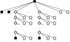
Figure 2: Structure of the subtree of rooted at a node .
White circles represent nodes in (so all their children are also white), gray circles - nodes in ,
and black circles - nodes in . Note, if is a child of then .
Consider a node . From the definition, has exactly one link
to a child in
that belongs to . If this child does not belong to , then it belongs to and the same argument can be repeated
for it. By following such links we eventually
get to a node in ; the first such node will be denoted as .
We will need two more definitions. For an index and patterns ending at position with we denote
(38a)
(38b)
We can now formulate the structure of the algorithm (see Algorithm 5).
Algorithm 5 Computing
1: initialize messages:
set
2: for each traverse nodes of tree
starting from the leaves and set
(39)
where
(40a)
(40b)
If then use
3: return
To fully specify the algorithm, we still need to describe how we compute quantities
and defined by eq. (40a) and (40b).
This is addressed by the theorem below.
Theorem 11.
(a) Algorithm 5 is correct.
(b) There holds .
(c) Let be the maximum depth of tree .
(Note, .)
With an preprocessing, values
for any with can be computed in time.
(d) Values for all can be computed in time,
or in time when .
Clearly, the theorem implies that the algorithm can be implemented in time,
or in time when .
To see this, observe that the sum in (40b) is effectively
over a subset of children of in the tree (see Fig. 2),
and this tree has size .
Before presenting the proof, let us make a few remarks.
To give some insights into how we prove the theorem, let us make a few remarks.
It can be easily checked that graph
has the following structure: the root has children,
and for each child the subtree
of rooted at is isomorphismic to the tree .
The isomorphism is given by the
the mapping .
For nodes with
we denote
to be the unique path from to in
(treated as a set of edges in ).
Analogously, for nodes with let
be the unique path from to in .
It follows from the previous paragraph that if
then path is isomorphic to the path .
The statement is equivalent to the correctness of (39).
Let us first divide the sum over in the last expression (39) into
two parts: nodes that belong to and those that do not:
(41)
It is easy to see that the second sum can be written as
(see Fig. 2), where
(42)
Using the distributive law, we can rewrite (39) as
(43)
We will use eq. (34) (for which the correctness is already proved) for the case when .
We can rewrite it as follows (we use the fact that ):
(44)
The first and the last terms of the sum in (44) equal to that
of the sum in (43). The lemma below implies
that the same holds for the second and third terms, thus proving the correctness of eq. (43).
Lemma 12.
(a) For any there holds
(45)
(b) For any there holds
(46)
Proof.
Part (a) Suppose that .
This means that
there are no patterns of the form
(recall that ). This in turn implies
that .
This also implies that for any there holds ,
and consequently .
Part (b) Suppose that .
The definition of implies that set does not contain nodes in
or in .
Using this fact and the definition of sets , we get the following.
(i)
If then .
(ii)
If then is a disjoint union of
and .
(iii)
Partial labeling
cannot end with a pattern .
(If such exists then from the fact above we get ,
i.e. and - a contradiction.)
Therefore, for such we have .
This implies that
.
Recall that .
Using this fact and properties (i)-(iii), we conclude that (46)
holds in each of the two cases ( and ).
∎
Let us consider the process of a breadth-first search in the tree starting from the root.
At each step we will keep a certain set of nodes of the tree (which we call active nodes), and the transition to the next step is made by choosing one of the active nodes and replacing it with its children. The process stops when the set of active nodes becomes equal to the set of the leaves of the tree.
To each step of the process we correspond a partition of the set . The partition is defined by the following rule: if are active nodes, then the partition is
.
Let us denote the partition at step as .
Partitions of the set is a poset with respect to the natural order defined as follows: if for any there is such that
.
It is easy to see that . Moreover, if a chosen active node at step is a special one and does not belong to then . Indeed, there are at least two children of , denoted as and ,
such that sets and are nonempty (by the definition of a special node).
As step these sets are separate components of partition ,
but at step these sets still belong to the same component of ; thus, .
We know that the length of a chain cannot exceed .
We conclude that the number of special patterns that do not belong to is bounded by ; this implies Theorem 11(b).
Note that . In this section we describe a preprocessing which will
allow computing values for any in time.
The procedure will be based on the following observation;
it follows trivially from the definition (38b).
Lemma 13.
For any there holds
(47)
During preprocessing we will compute values for pairs in
a certain set of size . In order to define , we need some notation.
For a pattern let be the height of in ,
and for an integer let be the node
of tree obtained from by taking steps towards the root. We now define
The preprocessing will consist of 3 steps.
Step 1: compute values for all .
We do it by traversing nodes of tree
and setting
(48)
This takes time.
Step 2: go through and compute
values for all
where is the set of children of in .
A naive way is to use the formula
for all ; however, this would take time where .
Instead, we do the following. Let us order patterns in arbitrarily:
. For denote
We compute these values in time by setting ,
and then using recursions
After that we set
For a given the procedure takes time,
and thus for all it takes time.
We now have values for all .
Step 3: compute values for all
using the recursion
for and .
Evaluating queries for We showed how to compute values for in time ;
let us now describe how to compute
value for a given in time .
Let us construct a sequence as follows:
, and for let where
is the maximum value such that for and is still
a descendant of . We stop when we get ; clearly, this happens after steps.
We now set
We will consider the general case of a commutative semiring and the case when ;
the latter will be called the MAP case.
Let for be the number of children of
in , ,
and for be the number
of children of in . We will present a
preprocessing
technique that will allow computing value for
in time . The resulting
complexity will be
In the MAP case (i.e. when )
we will present a faster solution. Namely, the preprocessing will take time,
and computing value for
will take
time, leading to the overall complexity .
For that we will use the Range Minimum Query (RMQ) problem
which is defined as follows: given numbers ,
compute for a given interval .
It is known [1] that with an preprocessing each
query for can be answered in time per interval.
As in the previous section, we denote .
We assume that for each
we already have values for all
(they were computed in the previous section).
Preprocessing Consider , and let us fix an ordering
of children of :
where .
For an interval we denote
(49)
The goal of preprocessing is to build a data structure that
we will allow an efficient computation of for any given interval .
In the MAP case we simply run the preprocessing of [1] for
the sequence ; this takes time.
Value for an interval can then be computed in time.
In the general case we do the following.
Define a set of intervals
Note that .
We compute quantities
for all . This can be done in time by
setting for and then using
recursions
for .
Value for an interval can now be
computed in time. Indeed, we can represent
as a disjoint union of intervals from :
with . We can then use the formula
(50)
Computing for
Denote .
As discussed earlier, (the set of children
of in ) is isomorphic to
.
Let be the ordering
of patterns in such that
is the ordering of patterns in
chosen in the preprocessing step. We need to compute
Denote .
We can represent as a disjoint union of at most intervals
where .
Clearly, (see Fig. 2),
and so .
We can write
(51)
As discussed above, each value can be computed
in time in the MAP case and in in the general case.
Thus, computing takes respectively
and time, as desired.
7 MAP for non-positive costs
In this section we assume that
and for all .
[2] gave an algorithm that makes comparisons
and additions. We will present a modification that
makes only comparisons. The number of additions
in general will still be , but we will show that
in certain scenarios it can be reduced using a Fast Fourier Transform (FFT).
We will assume that contains at least one word with
(it can always be added if needed).
As usual, we first select a set of patterns with ;
this step will be described later.
For a pattern let be the longest proper prefix of that is in
(, ). If does not contains proper prefixes of
then is undefined.
We can now present the algorithm.
Algorithm 6 Computing (if )
1: initialize messages: set
2: for traverse nodes of forest
starting from the leaves and set
(52)
where is the end position of (
and .
If is undefined then ignore the first expression in (52).
3: return
Selecting It remains to specify how to choose set . For patterns we define
A simple valid option is to set
.
Computing set is slightly more complicated, but can
still be done in polynomial time for a given (we omit this procedure).
In order to analyze set , let us define
As increases, set monotonically shrinks, and stops changing after .
We denote this limit set as , so that .
It can be seen that for all .
Complexity Assume that we use .
The algorithm performs two types of operations: comparisons
(to compute minima) and arithmetic operations (to compute the first expression in (52)).
The number of comparisons does not exceed the total number of edges in graphs
for , which is smaller than the number of nodes (since graphs are forests).
Thus, comparisons take time.
The time for arithmetic operations depends on how we compute quantities .
One possible approach is to use Lemma 1
for computing for all where
is the set of prefixes of patterns in (note that ).
We have , and therefore the resulting overall complexity
is .
Next, we describe an alternative approach based on a Fast Fourier Transform.
7.1 Computing using FFT
For a word and index let be the pattern .
It is easy to see that
Lemma 15.
For fixed words quantities for
can be computed in time.
Proof.
We assume that , otherwise the claim is trivial.
Let , and define sequences via
where is the Iverson bracket. It can be checked that
Thus, is the convolution of and the reverse of .
The convolution of such sequences can be computed in using a Fast Fourier Transform.
∎
In practice this method can be useful for computing when . A natural way to do this is first
choose a subset of words that are very often included as subwords in words from (usually, this
means where is some threshold constant). Then computing for all and
will take time.
For quantities can be computed directly.
An example of using such an approach is the following theorem; it is proved by taking and .
Theorem 16.
Suppose where consists of words of a fixed length . Then Algorithm 6 can be implemented in
time.
First, let us prove that for all patterns
there holds
(58)
We use induction on the order used in the algorithm.
The base case is ensured by the initialization step.
Consider pattern .
Suppose that is defined; let be the end position of .
Consider partial labeling , and let be its unique extension by letters
() such that .
Due to non-positivity of costs we have
Applying the induction hypothesis and the inequality above yields the desired claim:
where in the equations above always denotes a partial labeling in
and denotes a partial labeling in . If is undefined
then we can write similar inequalities but omitting expressions contaiting .
By applying the claim to patterns we conclude that .
The remainder of this section is devoted to the proof of the reverse inequality: .
Let us fix . Let
be the set of patterns present in , and
be the set of maximal patterns in .
We can assume w.l.o.g. that for each there exists with .
Indeed, if it is not the case for some then we can modify by replacing the -th letter of
with some letter ; this operation does not increase .
We define a total order on patterns as
the lexicographical order with components
(the first component is more significant).
Lemma 17.
(a) For each pattern there holds .
(b) Consider two consecutive patterns in
with , , and let
be the
pattern at which they intersect. (By the assumption above, ). There holds .
(c) For the patterns in (b), condition
implies .
Proof.
Part (a) We can write labeling as
where patterns , are empty.
Let us show that this choice satisfies conditions in (56). Condition (a) holds
since . Suppose that (b) does not
hold, then there exists pattern with .
We have
and thus - a contradiction. Therefore, .
Part (b)
The definitions of and imply
that . (If then we must have , but then - a contradiction.)
There also holds (otherwise we would have - a contradiction).
This means that we can write labeling as where
, and the pattern intervals are as follows:
Let us show that this choice satisfies conditions in (56). Condition (a) holds
since and . Suppose that (b) does not
hold, then there exists pattern where
and .
This means that .
From the definition of , there exists pattern
with . To summarize, we have and .
If then and thus - a contradiction.
Thus,
there must hold .
Similarly, we prove that .
This implies that ,
and therefore patterns and are not consecutive in - a contradiction.
Part (c) is a proper prefix of that belongs to .
Therefore, is defined.
We can define a sequence of patterns
with ,
respectively such that
and for . Let us prove by
induction on that for .
Let us first check the base of the induction. Since and ,
by the definition of graph there is a (unique) path
from to
with .
By eq. (52),
. Therefore,
where the last inequality holds by the assumption of part (c). This establishes the base case.
Now suppose that the claim holds for ; let us prove it for .
Denote and . Note, is the index in step 2 of the algorithm
during the processing of . From eq. (52) and the induction hypothesis
we get
We will prove next that ,
thus completing the induction step. It suffices to show that there is no
pattern with and .
Suppose on the contrary that such pattern exists. By the definition of there
exists pattern
with .
We have and .
These facts imply that ,
contradicting the assumption that and are consecutive
patterns in .
∎
We use induction on the total order . The lowest pattern
starts at position 1;
for such pattern the claim follows by inspecting Algorithm 6.
The induction step follows from Lemma 17(c).
∎
Acknowledgements
We thank Herbert Edelsbrunner for helpful discussions.
References
[1]
Omer Berkman and Uzi Vishkin.
Recursive star-tree parallel data structure.
SIAM Journal on Computing, 22(2):221–242, 1993.
[2]
N. Komodakis and N. Paragios.
Beyond pairwise energies: Efficient optimization for higher-order
MRFs.
In CVPR, 2009.
[3]
J. Lafferty, A. McCallum, and F Pereira.
Conditional random fields: Probabilistic models for segmenting and
labeling sequence data.
In ICML, 2001.
[4]
Viet Cuong Nguyen, Nan Ye, Wee Sun Lee, and Hai Leong Chieu.
Semi-Markov conditional random field with high-order features.
In ICML 2011 Structured Sparsity: Learning and Inference
Workshop, 2011.
[5]
Xian Qian, Xiaoqian Jiang, Qi Zhang, Xuanjing Huang, and Lide Wu.
Sparse higher order conditional random fields for improved sequence
labeling.
In ICML, 2009.
[6]
C. Rother, P. Kohli, W. Feng, and J. Jia.
Minimizing sparse higher order energy functions of discrete
variables.
In CVPR, 2009.
[7]
S. Sarawagi and W. Cohen.
Semi-Markov conditional random fields for information extraction.
In NIPS, 2004.
[8]
R. Takhanov and V. Kolmogorov.
Inference algorithms for pattern-based CRFs on sequence data.
In ICML, 2013.
[9]
M. D. Vose.
A linear algorithm for generating random numbers with a given
distribution.
IEEE Transactions on software engineering, 17(9):972–975,
1991.
[10]
Nan Ye, Wee Sun Lee, Hai Leong Chieu, and Dan Wu.
Conditional random fields with high-order features for sequence
labeling.
In NIPS, 2009.