Induced mirror symmetry breaking via template-controlled copolymerization: theoretical insights

Abstract

A chemical equilibrium model of template-controlled copolymerization is presented for describing the outcome of the experimental induced desymmetrization scenarios recently proposed by Lahav and coworkers.

It is an empirical fact that mirror symmetry is broken in all known biological systems, where processes crucial for life such as replication, imply chiral supramolecular structures, sharing the same chiral sign (homochirality). These chiral structures are proteins, composed of aminoacids almost exclusively found as the left-handed enantiomers (S), also DNA, and RNA polymers and sugars with chiral building blocks composed by right-handed (R) monocarbohydrates.

One scenario for the transition from prebiotic racemic chemistry to chiral biology suggests that homochiral peptides must have appeared before the onset of the primeval enzymes Bada and Miller (1987); Avetisov et al. (1985); Goldanskii et al. (1986); Avetisov and Goldanskii (1996); Orgel (1992). However, the polymerization of racemic mixtures (1:1 proportions) of monomers in ideal solutions typically yields chains composed of random sequences of both the left and right handed repeat units following a binomial distribution Guijarro and Yus (2009). This statistical problem has been overcome recently by the experimental demonstration of the generation of amphiphilic peptides of homochiral sequence, that is, of a single chirality, from racemic compositions. This route consists of two steps: (1) the formation of racemic parallel or anti-parallel $\beta$-sheets either in aqueous solution or in 3-D crystals Weissbuch et al. (2009) during the polymerization of racemic hydrophobic $\alpha$-amino acids followed by (2) an enantioselective controlled polymerization reaction Zepik et al. (2002); Nery et al. (2005, 2007); Rubinstein et al. (2007, 2008); Illos et al. (2008, 2010) (Fig. 1). This process leads to racemic or mirror-symmetric mixtures of isotactic oligopeptides where the chains are composed from amino acid residues of a single handedness. Furthermore, when racemic mixtures of different amino acid species were polymerized, isotactic co-peptides of homochiral sequence were generated. Here a host or majority species $(R_{0},S_{0})$, together with a given number $m$ of minority amino acid species $(R_{1},S_{1}),(R_{2},S_{2}),...(R_{m},S_{m})$ (supplied with lesser abundance) were employed. The guest (S) and (R) molecules are enantioselectively incorporated into the chains of the (S) and (R) peptides, respectively, however the former are stochastically distributed within the homochiral chains. As a combined result of these two effects, the sequence of the co-peptide S and R chains will differ from each other, resulting in non-racemic mixtures of co-peptide polymer chains: non-enantiomeric pairs of chains are thus formed. By considering the sequences of these peptide chains, a statistical departure from the racemic composition of the library of the peptide chains is created which varies with chain length $N$ and with the relative concentrations of the host/guest monomers used in the polymerization Nery et al. (2005, 2007).

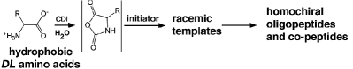
Figure 1: The scheme proposed in Ref. Weissbuch et al. (2009) leading to regio-enantioselection within racemic $\beta$-sheet templates.

The mechanism has some features in common with the scenarios proposed by GreenGreen and Garetz (1984), EschenmoserBolli et al. (1997) and SiegelSiegel (1998) in which a limited supply of material results in a stochastic mirror symmetry breaking process.

To address the general scenario for the generation of libraries of diastereoisomeric mixtures of peptides in accord with that proposed in Ref.Nery et al. (2005), consider a model with a host amino acid species and $m$ guest amino acids. We assume as given the prior formation of the initial templates or $\beta$-sheets, and are concerned exclusively with the subsequent random polymerization reactions (step (2)). The underlying nonlinear template control is implicit throughout the discussion.

We consider stepwise additions and dissociations of single monomers from one end of the (co)polymer chain, considered as a strand within the $\beta$-sheet. It is reasonable to regard the $\beta$-sheet in equilibrium with the free monomer poolWagner et al. (2011).

From detailed balance, each individual monomer attachment or dissociation reaction is in equilibrium. This holds for closed equilibrium systems in which the free monomers are depleted/replenished by the templated polymerization. Then we can compute the equilibrium concentrations of all the (co)-polymers in terms of equilibrium constants $K_{i}$ and the free monomer concentrations. The equilibrium concentration of an $S$-type copolymer chain of length $n_{0}+n_{1}+n_{2}+...+n_{m}=N$ made up of $n_{j}$ molecules $S_{j}$ is given by $p^{S}_{n_{0},n_{1},...,n_{m}}=(K_{0}s_{0})^{n_{0}}(K_{1}s_{1})^{n_{1}}...(K_{m}s_{m})^{n_{m}}/K_{0}$, where $s_{j}=[S_{j}]$ Markvoort et al. (2011). Similarly for the concentration of an $R$-type copolymer chain of length $n^{\prime}_{0}+n^{\prime}_{1}+n^{\prime}_{2}+...+n^{\prime}_{m}=N$ made up of $n^{\prime}_{j}$ molecules $R_{j}$: $p^{R}_{n^{\prime}_{0},n^{\prime}_{1},...,n^{\prime}_{m}}=(K_{0}r_{0})^{n^{\prime}_{0}}(K_{1}r_{1})^{n^{\prime}_{1}}...(K_{m}r_{m})^{n^{\prime}_{m}}/K_{0}$, where $r_{j}=[R_{j}]$.

The number of different $S$-type copolymers of length $l$ with $n_{j}$ molecules of type $S_{j}$ is given by the multinomial coefficient. Hence the total concentration of the $S$-type copolymers of length $l$ is given by

$$p_{l}^{S} = \sum_{n_{0}+n_{1}+...+n_{m}=l}\left(\begin{array}[]{c}l\\ n_{0},n_{1},...,n_{m}\\ \end{array}\right)p^{S}_{n_{0},n_{1},...,n_{m}}=\frac{1}{K_{0}}(K_{0}s_{0}+K_{1}s_{1}+...+K_{m}s_{m})^{l},$$ (3)

which follows from the multinomial theorem nis (technical report). We calculate the number of each type $S_{j}$ of $S$-monomer present in the $S$-copolymer of length equal to $l$, for any $0\leq j\leq m$:

$$s_{j}(p^{S}_{l})=\sum_{n_{0}+n_{1}+...+n_{m}=l}\left(\begin{array}[]{c}l\\ n_{0},n_{1},...,n_{m}\\ \end{array}\right)n_{j}p^{S}_{n_{0},n_{1},...,n_{m}}=s_{j}\frac{\partial}{\partial s_{j}}p_{l}^{S}=\frac{K_{j}}{K_{0}}s_{j}l(K_{0}s_{0}+K_{1}s_{1}+...+K_{m}s_{m})^{l-1}.$$ (6)

Then we need to know the total amount of the $S$-type monomers bound within the $S$-type copolymers, from the dimer on up to a maximum chain length $N$. Using Eq.6 for the $jth$ type of amino acid, this is given by

$$s_{j}(p^{S}_{Tot})=\sum_{l=2}^{N}s_{j}(p^{S}_{l})\rightarrow\frac{K_{j}}{K_{0}}s_{j}\frac{a(2-a)}{(1-a)^{2}},$$ (7)

the final expression holds in the limit $N\rightarrow\infty$ provided that $a=(K_{0}s_{0}+K_{1}s_{1}+...+K_{m}s_{m})<1$. This must be the case, otherwise the system would contain an infinite number of molecules Markvoort et al. (2011). Similar considerations hold for the $R$-sector, and the total amount of $R$ monomers inside $R$ type copolymers for the $jth$ amino acid, is given by $r_{j}(p^{R}_{Tot})=\frac{K_{j}}{K_{0}}r_{j}\frac{b(2-b)}{(1-b)^{2}}$ where $b=(K_{0}r_{0}+K_{1}r_{1}+...+K_{m}r_{m})<1$. From this we obtain the mass balance equations which hold for both enantiomers of the host and guest amino acids, and is our key result:

$$s_{j}+\frac{K_{j}}{K_{0}}s_{j}\frac{a(2-a)}{(1-a)^{2}}={s_{j}}_{tot},\qquad r_{j}+\frac{K_{j}}{K_{0}}r_{j}\frac{b(2-b)}{(1-b)^{2}}={r_{j}}_{tot}.$$ (8)

These equations express the fact that each type of enantiomer is either free, or is else bound inside a (co)polymer strand within the template.

The problem then consists in the following: given the total concentrations of all the $m+1$ enantiomers $\{{s_{j}}_{tot},{r_{j}}_{tot}\}_{j=0}^{m}$, and the $K_{i}$ we calculate the free monomer concentrations $\{s_{j},r_{j}\}_{j=0}^{m}$ from solving Eqs. (9). Denote by $s_{0_{tot}}+...+s_{m_{tot}}+r_{0_{tot}}+...+r_{m_{tot}}=c_{tot}$ the total system concentration. From the solutions we can calculate e.g., the equilibrium concentrations of homochiral copolymers of any specific sequence or composition as well as the resultant enantiomeric excess for homochiral chains of length $l$ composed of the host (majority) amino acid: $ee_{l}=\frac{(r_{0})^{l}-(s_{0})^{l}}{(r_{0})^{l}+(s_{0})^{l}}$. When there are no guest aminoacids, i.e., for $m=0$, and when the majority species is supplied in racemic proportions ${s_{0}}_{tot}:{r_{0}}_{tot}=1:1$, then $ee_{l}$ must be zero: there will be no mirror symmetry breaking. So we turn to the scenario of RefNery et al. (2005) and consider the influence of a single guest species, $m=1$ being sufficient for our purposes.

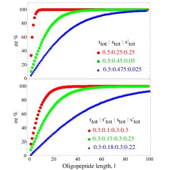
Figure 2: Calculated $ee$ values versus chain length $l$ from solving Eqs. (9). Top: non-racemic host $r_{tot}>s_{tot}$ and one guest aminoacid $s^{\prime}_{tot}$ $(m=1)$ and three monomer starting compositions (in moles) $r_{tot}:s_{tot}:s^{\prime}_{tot}=0.5:0.25:0.25$ (filled circles), $0.5:0.45:0.05$ (squares) and $0.5:0.475:0.025$ (triangles) for the equilibrium constant $K=1M^{-1}$ and the total monomer concentration $c_{tot}=1M$. Compare to Fig. 13 of Ref.Nery et al. (2005). Bottom: racemic host $r_{tot}=s_{tot}$ and $m=1$ guest $r^{\prime}_{tot},s^{\prime}_{tot}$. Starting compositions $r_{tot}:r^{\prime}_{tot}:s_{tot}:s^{\prime}_{tot}=0.3:0.1:0.3:0.3$ (filled circles), $0.3:0.15:0.3:0.25$ (squares) and $0.3:0.18:0.3:0.22$ (triangles) for four monomers.

We first use our mass balance equations to calculate $ee_{l}$ for the same initial compositions of the monomers as reported in Nery et al. (2005). This is shown in top of Fig. 2. We consider a single equilibrium constant $K_{0}=K_{1}=K=1M^{-1}$ for sake of simplicity, and the total system concentration, $c_{tot}=1M$. The enantiomeric excess increases when increasing the amount of guest species $s^{\prime}_{tot}$, obtaining a maximal symmetry breaking for the case shown with equal amounts of majority and minority S-molecules: $s_{tot}=s^{\prime}_{tot}$. In the limit as $s^{\prime}_{tot}\rightarrow 0$ we tend towards a racemic situation, so decreasing the amount of the minority or guest species is equivalent to approaching the racemic state, manifested through ever smaller values of $ee_{l}$ for fixed $l$ (top to bottom sequence of curves). The $ee_{l}$ increases monotonically with the chain length $l$ in all cases. The behavior of the $ee_{l}$ demonstrates quite well the induced symmetry breaking mechanism proposed in Ref.Nery et al. (2005).

The solutions of the mass balance equations (9) can be used to evaluate the average chain lengths as functions of initial monomer compositions and the equilibrium constants. The average chain lengths of the $S$-type copolymers $<l_{S}>$, composed of random sequences of the $S_{j}$ type monomers, and that of the $R$-type copolymers $<l_{R}>$ composed of random sequences of the $R_{j}$ type monomers, are derived in the Supplementary Information. Results for the $m=1$ three monomer cases are shown there in Table I. There is a marked increase in the average chain length when increasing $K$, we moreover observe how the average chain length corresponding to each monomer species increases when increasing its own starting proportion. In the case of additives of only one handedness (three monomer case) and for the different compositions considered ($r_{tot}:s_{tot}:s^{\prime}_{tot}=0.5:0.25:0.25$, $0.5:0.45:0.05$, $0.5:0.475:0.025$) the average chain length for the $S$-type copolymers and the $R$-type polymers will be the same. This follows since $K$ is the same for both monomer types and the amount of $S$-type and $R$-type molecules in the starting compositions is the same, $r_{tot}=s_{tot}+s^{\prime}_{tot}$, so the average chain length must be the same: $<l_{S}>=<l_{R}>$.

By a further example, we carry out an analysis for the case of one guest $m=1$ and all four enantiomers, treating a majority species $R,S$ in strictly racemic proportions and a single guest amino acid $R^{\prime},S^{\prime}$ in various relative proportions. We solve Eq. (9) and then calculate $ee_{l}$ for the different chain lengths $l$ for three different starting monomer compositions. In Fig. 2 (bottom) we show the results obtained from calculating $ee_{l}$ for $K=1M^{-1}$ and $c_{tot}=1M$. The behavior is qualitatively similar to that previously commented, the greater the relative disproportion of the minority species $r^{\prime}_{tot},s^{\prime}_{tot}$, the greater is the enantiomeric excess. Values for the average chain lengths are calculated for four molecules, with the abundances $r_{tot}:r^{\prime}_{tot}:s_{tot}:s^{\prime}_{tot}=0.3:0.1:0.3:0.3$ and $r_{tot}:r^{\prime}_{tot}:s_{tot}:s^{\prime}_{tot}=0.3,0.14,0.3:0.26$, and are displayed in Table II in Supplementary Information, where other choices for the $K_{i}$ and $c_{tot}$ are employed (see Tables III-VI).

In summary, we consider a multinomial sample space for the distribution of equilibrium concentrations of homochiral copolymers formed via template control. We deduce mass balance equations for the enantiomers of the individual amino acid species, and their solutions are used to evaluate the sequence-dependent copolymer concentrations, in terms of the total species concentrations. Measurable quantities signalling the degree of mirror symmetry breaking such as the $ee$ and average chain lengths are evaluated. This approach provides a quantitative basis for the template-controlled induced desymmetrization mechanisms advocated by Lahav and coworkers Zepik et al. (2002); Nery et al. (2005, 2007); Rubinstein et al. (2007, 2008); Illos et al. (2008, 2010).

We are indebted to Meir Lahav for suggesting a mathematical approach to this problem. CB has a Calvo Rodés scholarship from INTA. DH acknowledges a grant AYA2009-13920-C02-01 from the MICINN and forms part of the COST Action CM0703 “Systems Chemistry”.

Supplementary Information

I $\beta$-sheet controlled copolymerization

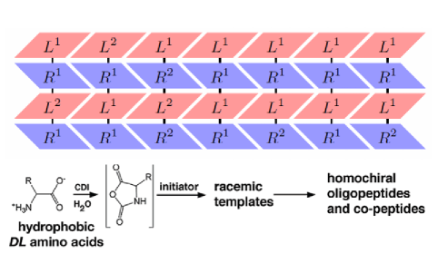
Figure 3: Regio-enantioselection within racemic $\beta$-sheet templates.

The proposed regio-enantioselection within racemic beta sheets is graphically illustrated by Fig 3. For sake of simplicity, we consider a host majority species $(L_{1},R_{1})$ and a minority guest species $(L_{2},R_{2}$) of amino acids both provided in ideally racemic proportions. The amino acids of a given handedness attach to sites of the same chirality within the growing beta sheet leading to the polymerization of oligomer strands of a single chirality, in the alternating fashion as depicted. The vertical line segments denote hydrogen bonds between adjacent strands. Since the polymerization in any given strand is random and the guest molecules are less abundant than the hosts, the former will attach in a random fashion, leading to independent uncorrelated random sequences in each strand. The overall effect leads to non-enantiomeric pairs of chiral copolymers, so mirror symmetry is broken in a stochastic manner.

II Average chain lengths

We can calculate the average copolymer chain lengths as functions of initial monomer compositions ${s_{j}}_{tot},{r_{j}}_{tot}$, for the $jth$ species, $0\leq j\leq m$, and the equilibrium constants $K_{j}$, using the solutions of our mass balance equations:

$$s_{j}+\frac{K_{j}}{K_{0}}s_{j}\frac{a(2-a)}{(1-a)^{2}}={s_{j}}_{tot},\qquad r_{j}+\frac{K_{j}}{K_{0}}r_{j}\frac{b(2-b)}{(1-b)^{2}}={r_{j}}_{tot},$$ (9)

where $a=K_{0}s_{0}+K_{1}s_{1}+...+K_{m}s_{m}<1$ and $b=K_{0}r_{0}+K_{1}r_{1}+...+K_{m}r_{m}<1$.

The ensemble-averaged chain lengths afford an alternative measure of the degree of mirror symmetry breaking resulting from the desymmetrization process discussed in Nery et al. (2005). There are a number of relevant and interesting averages one can define and calculate. The average chain lengths, starting from the dimers, of the $S$-type copolymers, composed of random sequences of the $S_{j}$ type monomers, and that of the $R$-type copolymers composed of random sequences of the $R_{j}$ type monomers are given by:

$$<l_{S}>=\frac{\sum_{l=2}^{N}(s_{0}(p^{S}_{l})+s_{1}(p^{S}_{l})+...+s_{m}(p^{S}_{l}))}{\sum_{l=2}^{N}p^{S}_{l}}\rightarrow\frac{(s_{0}+\frac{K_{1}}{K_{0}}s_{1}+...+\frac{K_{m}}{K_{0}}s_{m})\frac{a(2-a)}{(1-a)^{2}}}{\frac{a^{2}}{(1-a)K_{0}}}=\frac{2-a}{1-a},$$ (10)

$$<l_{R}>=\frac{\sum_{l=2}^{N}(r_{0}(p^{R}_{l})+r_{1}(p^{R}_{l})+...+r_{m}(p^{R}_{l}))}{\sum_{l=2}^{N}p^{R}_{l}}\rightarrow\frac{(r_{0}+\frac{K_{1}}{K_{0}}r_{1}+...+\frac{K_{m}}{K_{0}}r_{m})\frac{b(2-b)}{(1-b)^{2}}}{\frac{b^{2}}{(1-b)K_{0}}}=\frac{2-b}{1-b},$$ (11)

respectively. We also obtain an expression for the average length of the polymer chains composed exclusively by the $S_{j}$ or $R_{j}$ monomers for a given fixed amino acid type $j$:

$$<l_{S}^{s_{j}}>=\frac{\sum_{l=2}^{N}s_{j}(p^{S(s_{j})}_{l})}{\sum_{l=2}^{N}p^{S(s_{j})}_{l}}=\frac{\sum_{l=2}^{N}\frac{K_{j}}{K_{0}}s_{j}l(K_{j}s_{j})^{l-1}}{\sum_{l=2}^{N}\frac{(K_{j}s_{j})^{l}}{K_{0}}}\rightarrow\frac{\frac{(s_{j}K_{j})^{2}(2-K_{j}s_{j})}{(1-K_{j}s_{j})^{2}}}{\frac{(K_{j}s_{j})^{2}}{(1-K_{j}s_{j})}}=\frac{2-K_{j}s_{j}}{1-K_{j}s_{j}},$$ (12)

$$<l_{R}^{r_{j}}>=\frac{\sum_{l=2}^{N}r_{j}(p^{R(r_{j})}_{l})}{\sum_{l=2}^{N}p^{R(r_{j})}_{l}}=\frac{\sum_{l=2}^{N}\frac{K_{j}}{K_{0}}r_{j}l(K_{j}r_{j})^{l-1}}{\sum_{l=2}^{N}\frac{(K_{j}r_{j})^{l}}{K_{0}}}\rightarrow\frac{\frac{(r_{j}K_{j})^{2}(2-K_{j}r_{j})}{(1-K_{j}r_{j})^{2}}}{\frac{(K_{j}r_{j})^{2}}{(1-K_{j}r_{j})}}=\frac{2-K_{j}r_{j}}{1-K_{j}r_{j}}.$$ (13)

To complete the list, we can calculate the chain length averaged over all the copolymers in the system:

$$<l> = \frac{\sum_{l=2}^{N}(s_{0}(p^{S}_{l})+s_{1}(p^{S}_{l})+...+s_{m}(p^{S}_{l})+r_{0}(p^{R}_{l})+r_{1}(p^{R}_{l})+...+r_{m}(p^{R}_{l}))}{\sum_{l=2}^{N}(p^{S}_{l}+p^{R}_{l})}$$ (14)

$$\rightarrow \frac{(s_{0}+\frac{K_{1}}{K_{0}}s_{1}+...+\frac{K_{m}}{K_{0}}s_{m})\frac{a(2-a)}{(1-a)^{2}}+(r_{0}+\frac{K_{1}}{K_{0}}r_{1}+...+\frac{K_{m}}{K_{0}}r_{m})\frac{b(2-b)}{(1-b)^{2}}}{\frac{a^{2}}{(1-a)K_{0}}+\frac{b^{2}}{(1-b)K_{0}}}$$

$$= \frac{a^{2}(2-a)(1-b)^{2}+b^{2}(2-b)(1-a)^{2}}{a^{2}(1-b)^{2}(1-a)+b^{2}(1-b)(1-a)^{2}}.$$

The right-hand most expressions $(\rightarrow)$ hold in the limit of $N\rightarrow\infty$ and for $a<1$ and $b<1$.

In the following, we first consider the simplest case of $m=1$ guest and equal equilibrium constants $K_{0}=K_{1}=K$. In the case of additives of only one handedness (chiral additives, $r_{tot}:s_{tot}:s^{\prime}_{tot}$), and for the three different cases considered in the Communication ($0.5:0.25:0.25$, $0.5:0.45:0.05$ and $0.5:0.475:0.025$) the average chain length for the $S$-type copolymers and the $R$-type polymers will be the same, see Table 1. This follows since the equilibrium constant is the same for both monomer types and the amount of $S$-type and $R$-type molecules in the starting compositions is the same $r_{tot}=s_{tot}+s^{\prime}_{tot}$, so the total average chain length must be the same: $<l_{S}>=<l_{R}>=<l>$. In the particular case of $r_{tot}:s_{tot}:s^{\prime}_{tot}=0.5:0.25:0.25$, that is, for the same starting amounts $s_{tot}=s^{\prime}_{tot}$, the average length for the chains exclusively composed of $S$ or $S^{\prime}$ is the also same: $<l_{S}^{s}>=<l_{S}^{s^{\prime}}>$ (fifth and sixth columns in Table 1). We can appreciate a clear increase in the average chain length when increasing $K$ (top to bottom rows), we observe moreover that the average chain length corresponding to each monomer species increases when increasing its starting proportion; see Table 1, from left to right in the groups.

Table 1:  Average chain lengths for the three different starting compositions as a function of $K$ for $c_{tot}=1M$

	$r_{tot}:s_{tot}:s^{\prime}_{tot}=0.5:0.25:0.25$					$r_{tot}:s_{tot}:s^{\prime}_{tot}=0.5:0.45:0.05$					$r_{tot}:s_{tot}:s^{\prime}_{tot}=0.5:0.475:0.025$
$K(M^{-1})$	$<l>$	$<l_{S}>$	$<l_{R}>$	$<l_{S}^{s}>$	$<l_{S}^{s^{\prime}}>$	$<l>$	$<l_{S}>$	$<l_{R}>$	$<l_{S}^{s}>$	$<l_{S}^{s^{\prime}}>$	$<l>$	$<l_{S}>$	$<l_{R}>$	$<l_{S}^{s}>$	$<l_{S}^{s^{\prime}}>$
$1$	$2.37$	$2.37$	$2.37$	$2.15$	$2.15$	$2.37$	$2.37$	$2.37$	$2.32$	$2.03$	$2.37$	$2.37$	$2.37$	$2.34$	$2.01$
$5$	$3.16$	$3.16$	$3.16$	$2.37$	$2.37$	$3.16$	$3.16$	$3.16$	$2.93$	$2.06$	$3.16$	$3.16$	$3.16$	$3.04$	$2.03$
$10$	$3.79$	$3.79$	$3.79$	$2.47$	$2.47$	$3.79$	$3.79$	$3.79$	$3.37$	$2.07$	$3.79$	$3.79$	$3.79$	$3.56$	$2.03$
$50$	$6.52$	$6.52$	$6.52$	$2.69$	$2.69$	$6.52$	$6.52$	$6.52$	$4.80$	$2.09$	$6.52$	$6.52$	$6.52$	$5.51$	$2.04$
$100$	$8.59$	$8.59$	$8.59$	$2.77$	$2.77$	$8.59$	$8.59$	$8.59$	$5.57$	$2.10$	$8.59$	$8.59$	$8.59$	$6.71$	$2.05$
$500$	$17.32$	$17.32$	$17.32$	$2.88$	$2.88$	$17.32$	$17.32$	$17.32$	$7.44$	$2.10$	$17.32$	$17.32$	$17.32$	$10.24$	$2.05$
$1000$	$23.87$	$23.87$	$23.87$	$2.92$	$2.92$	$23.87$	$23.87$	$23.87$	$8.18$	$2.11$	$23.87$	$23.87$	$23.87$	$11.92$	$2.05$

In the particular case of $r_{tot}:r^{\prime}_{tot}:s_{tot}:s^{\prime}_{tot}=0.3:0.1:0.3:0.3$, that is the same starting amounts of $r$, $s$ and $s^{\prime}$, the average chain length for the chains exclusively composed of $s$ or $s^{\prime}$ is the same, $<l_{S}^{s}>=<l_{S}^{s^{\prime}}>$. Numerical results for the cases $r_{tot}:r^{\prime}_{tot}:s_{tot}:s^{\prime}_{tot}=0.3:0.1:0.3:0.3$ and $r_{tot}:r^{\prime}_{tot}:s_{tot}:s^{\prime}_{tot}=0.3,0.14,0.3:0.26$ are shown in Table 2.

We consider the effect of different equilibrium constants $K_{0}\neq K_{1}$ and a much smaller total system concentration $c_{tot}=10^{-3}M$ in Table 3. The dependence on varying $c_{tot}$ for fixed but distinct equilibrium constants $K_{0}\neq K_{1}$ is displayed in Table 4. These should be compared to the previous Table 1, since they refer to the same starting monomer compositions as used in that Table. Finally Tables 5 and 6 have been calculated for the same starting compositions as Table 2 and can be compared with the latter.

Table 2:  Average chain lengths for the two different starting compositions as a function of $K$ for $c_{tot}=1M$

	$r_{tot}:r^{\prime}_{tot}:s_{tot}:s^{\prime}_{tot}=0.3:0.1:0.3:0.3$							$r_{tot}:r^{\prime}_{tot}:s_{tot}:s^{\prime}_{tot}=0.3:0.14:0.3:0.26$
$K(M^{-1})$	$<l>$	$<l_{S}>$	$<l_{R}>$	$<l_{S}^{s}>$	$<l_{S}^{s^{\prime}}>$	$<l_{R}^{r}>$	$<l_{R}^{r^{\prime}}>$	$<l>$	$<l_{S}>$	$<l_{R}>$	$<l_{S}^{s}>$	$<l_{S}^{s^{\prime}}>$	$<l_{R}^{r}>$	$<l_{R}^{r^{\prime}}>$
$1$	$2.38$	$2.42$	$2.31$	$2.17$	$2.17$	$2.21$	$2.06$	$2.37$	$2.40$	$2.33$	$2.18$	$2.15$	$2.20$	$2.08$
$5$	$3.18$	$3.30$	$3.00$	$2.40$	$2.40$	$2.60$	$2.14$	$3.16$	$3.25$	$3.07$	$2.42$	$2.35$	$2.54$	$2.20$
$10$	$3.82$	$4.00$	$3.56$	$2.50$	$2.50$	$2.84$	$2.18$	$3.80$	$3.92$	$3.66$	$2.54$	$2.43$	$2.74$	$2.25$
$50$	$6.57$	$7.00$	$6.00$	$2.71$	$2.71$	$3.50$	$2.25$	$6.54$	$6.82$	$6.22$	$2.80$	$2.62$	$3.23$	$2.35$
$100$	$8.64$	$9.26$	$7.84$	$2.78$	$2.78$	$3.78$	$2.27$	$8.61$	$9.00$	$8.15$	$2.88$	$2.68$	$3.42$	$2.38$
$500$	$17.41$	$18.83$	$15.65$	$2.89$	$2.89$	$4.32$	$2.30$	$17.35$	$18.24$	$16.34$	$3.02$	$2.78$	$3.76$	$2.42$
$1000$	$24.00$	$26.00$	$21.50$	$2.92$	$2.92$	$4.49$	$2.31$	$23.91$	$25.17$	$22.48$	$3.06$	$2.80$	$3.86$	$2.44$

Table 3:  Average chain lengths for the three different starting compositions as a function of $K_{0}$ for $K_{1}=K_{0}/2$ and $c_{tot}=10^{-3}M$

	$r_{tot}:s_{tot}:s^{\prime}_{tot}=0.5:0.25:0.25$					$r_{tot}:s_{tot}:s^{\prime}_{tot}=0.5:0.45:0.05$					$r_{tot}:s_{tot}:s^{\prime}_{tot}=0.5:0.475:0.025$
$K_{0}(M^{-1})$	$<l>$	$<l_{S}>$	$<l_{R}>$	$<l_{S}^{s}>$	$<l_{S}^{s^{\prime}}>$	$<l>$	$<l_{S}>$	$<l_{R}>$	$<l_{S}^{s}>$	$<l_{S}^{s^{\prime}}>$	$<l>$	$<l_{S}>$	$<l_{R}>$	$<l_{S}^{s}>$	$<l_{S}^{s^{\prime}}>$
$1$	$2.00$	$2.00$	$2.00$	$2.00$	$2.00$	$2.00$	$2.00$	$2.00$	$2.00$	$2.00$	$2.00$	$2.00$	$2.00$	$2.00$	$2.00$
$10$	$2.00$	$2.00$	$2.00$	$2.00$	$2.00$	$2.00$	$2.00$	$2.00$	$2.00$	$2.00$	$2.00$	$2.00$	$2.00$	$2.00$	$2.00$
$100$	$2.04$	$2.04$	$2.05$	$2.02$	$2.01$	$2.05$	$2.05$	$2.05$	$2.04$	$2.00$	$2.05$	$2.05$	$2.05$	$2.04$	$2.00$
$1000$	$2.34$	$2.31$	$2.37$	$2.17$	$2.10$	$2.36$	$2.36$	$2.37$	$2.32$	$2.02$	$2.36$	$2.36$	$2.37$	$2.34$	$2.00$
$10000$	$3.76$	$3.73$	$3.79$	$2.51$	$2.42$	$3.79$	$3.78$	$3.80$	$3.40$	$2.06$	$3.79$	$3.79$	$3.79$	$3.58$	$2.03$
$100000$	$8.57$	$8.56$	$8.59$	$2.78$	$2.75$	$8.59$	$8.58$	$8.59$	$5.60$	$2.10$	$8.59$	$8.59$	$8.59$	$6.73$	$2.04$

Table 4:  Average chain lengths for the three different starting compositions as a function of $c_{tot}$ for $K_{0}=100000$ and $K_{1}=K_{0}/2$

	$r_{tot}:s_{tot}:s^{\prime}_{tot}=0.5:0.25:0.25$					$r_{tot}:s_{tot}:s^{\prime}_{tot}=0.5:0.45:0.05$					$r_{tot}:s_{tot}:s^{\prime}_{tot}=0.5:0.475:0.025$
$c_{tot}(M)$	$<l>$	$<l_{S}>$	$<l_{R}>$	$<l_{S}^{s}>$	$<l_{S}^{s^{\prime}}>$	$<l>$	$<l_{S}>$	$<l_{R}>$	$<l_{S}^{s}>$	$<l_{S}^{s^{\prime}}>$	$<l>$	$<l_{S}>$	$<l_{R}>$	$<l_{S}^{s}>$	$<l_{S}^{s^{\prime}}>$
$10^{-5}$	$2.34$	$2.31$	$2.37$	$2.17$	$2.10$	$2.36$	$2.36$	$2.36$	$2.32$	$2.02$	$2.36$	$2.36$	$2.37$	$2.34$	$2.01$
$10^{-4}$	$3.76$	$3.73$	$3.79$	$2.51$	$2.42$	$3.79$	$3.78$	$3.79$	$3.40$	$2.06$	$3.79$	$3.79$	$3.79$	$3.58$	$2.03$
$10^{-3}$	$8.57$	$8.56$	$8.59$	$2.78$	$2.75$	$8.59$	$8.58$	$8.59$	$5.60$	$2.09$	$8.59$	$8.59$	$8.59$	$6.73$	$2.04$
$10^{-2}$	$23.86$	$23.86$	$23.87$	$2.92$	$2.91$	$23.87$	$23.86$	$23.87$	$8.18$	$2.11$	$23.87$	$23.87$	$23.87$	$11.93$	$2.05$
$10^{-1}$	$72.21$	$72.21$	$72.21$	$2.97$	$2.97$	$72.22$	$72.22$	$72.21$	$9.88$	$2.11$	$72.24$	$72.27$	$72.21$	$16.79$	$2.05$

Table 5:  Average chain lengths for the two different starting compositions as a function of $K_{0}$ for $K_{1}=K_{0}/2$ and $c_{tot}=10^{-3}M$

	$r_{tot}:r^{\prime}_{tot}:s_{tot}:s^{\prime}_{tot}=0.3:0.1:0.3:0.3$							$r_{tot}:r^{\prime}_{tot}:s_{tot}:s^{\prime}_{tot}=0.3:0.14:0.3:0.26$
$K_{0}(M^{-1})$	$<l>$	$<l_{S}>$	$<l_{R}>$	$<l_{S}^{s}>$	$<l_{S}^{s^{\prime}}>$	$<l_{R}^{r}>$	$<l_{R}^{r^{\prime}}>$	$<l>$	$<l_{S}>$	$<l_{R}>$	$<l_{S}^{s}>$	$<l_{S}^{s^{\prime}}>$	$<l_{R}^{r}>$	$<l_{R}^{r^{\prime}}>$
$1$	$2.00$	$2.00$	$2.00$	$2.00$	$2.00$	$2.00$	$2.00$	$2.00$	$2.00$	$2.00$	$2.00$	$2.00$	$2.00$	$2.00$
$10$	$2.00$	$2.00$	$2.00$	$2.00$	$2.00$	$2.00$	$2.00$	$2.00$	$2.00$	$2.00$	$2.00$	$2.00$	$2.00$	$2.00$
$100$	$2.04$	$2.04$	$2.03$	$2.03$	$2.01$	$2.03$	$2.00$	$2.04$	$2.04$	$2.04$	$2.03$	$2.01$	$2.03$	$2.00$
$1000$	$2.33$	$2.36$	$2.28$	$2.19$	$2.12$	$2.22$	$2.04$	$2.33$	$2.35$	$2.30$	$2.20$	$2.10$	$2.22$	$2.05$
$10000$	$3.77$	$3.94$	$3.53$	$2.53$	$2.45$	$2.88$	$2.16$	$3.75$	$3.86$	$3.61$	$2.58$	$2.40$	$2.78$	$2.22$
$100000$	$8.62$	$9.23$	$7.83$	$2.80$	$2.77$	$3.81$	$2.27$	$8.58$	$8.79$	$8.13$	$2.89$	$2.67$	$3.44$	$2.37$

Table 6:  Average chain lengths for the two different starting compositions as a function of $c_{tot}$ for $K_{0}=100000$ and $K_{1}=K_{0}/2$

	$r_{tot}:r^{\prime}_{tot}:s_{tot}:s^{\prime}_{tot}=0.3:0.1:0.3:0.3$							$r_{tot}:r^{\prime}_{tot}:s_{tot}:s^{\prime}_{tot}=0.3:0.14:0.3:0.26$
$c_{tot}(M)$	$<l>$	$<l_{S}>$	$<l_{R}>$	$<l_{S}^{s}>$	$<l_{S}^{s^{\prime}}>$	$<l_{R}^{r}>$	$<l_{R}^{r^{\prime}}>$	$<l>$	$<l_{S}>$	$<l_{R}>$	$<l_{S}^{s}>$	$<l_{S}^{s^{\prime}}>$	$<l_{R}^{r}>$	$<l_{R}^{r^{\prime}}>$
$10^{-5}$	$2.33$	$2.36$	$2.28$	$2.19$	$2.12$	$2.22$	$2.04$	$2.33$	$2.35$	$2.30$	$2.20$	$2.10$	$2.22$	$2.05$
$10^{-4}$	$3.77$	$3.94$	$3.53$	$2.53$	$2.45$	$2.88$	$2.16$	$3.75$	$3.86$	$3.61$	$2.58$	$2.40$	$2.78$	$2.22$
$10^{-3}$	$8.62$	$9.23$	$7.83$	$2.79$	$2.77$	$3.81$	$2.26$	$8.58$	$8.97$	$8.13$	$2.89$	$2.67$	$3.44$	$2.37$
$10^{-2}$	$23.99$	$25.99$	$21.50$	$2.92$	$2.92$	$4.49$	$2.31$	$23.90$	$25.16$	$22.48$	$3.06$	$2.80$	$3.86$	$2.43$
$10^{-1}$	$72.58$	$78.96$	$64.75$	$2.97$	$2.97$	$4.82$	$2.33$	$72.34$	$76.33$	$67.83$	$3.12$	$2.85$	$4.05$	$2.46$

References

• Bada and Miller (1987) J. Bada and S. Miller, Biosystems 20, 21 (1987).
• Avetisov et al. (1985) V. Avetisov, V. Goldanskii, and V. Kuzmin, Dokl. Akad. Nauk USSR 115, 282 (1985).
• Goldanskii et al. (1986) V. Goldanskii, V. Avetisov, and V. Kuzmin, FEBS Lett. 207, 181 (1986).
• Avetisov and Goldanskii (1996) V. Avetisov and V. Goldanskii, Proc. Natl. Acad. Sci. USA 93, 11435 (1996).
• Orgel (1992) L. Orgel, Nature 358, 203 (1992).
• Guijarro and Yus (2009) A. Guijarro and M. Yus, The Origin of Chirality in the Molecules of Life (RSC Publishing, Cambridge, 2009), 1st ed.
• Weissbuch et al. (2009) I. Weissbuch, R. Illos, G. Bolbach, and M. Lahav, Acc. Chem. Res. 42, 1128 (2009).
• Zepik et al. (2002) H. Zepik, E. Shavit, M. Tang, T. Jensen, K. Kjaer, G. Bolbach, L. Leiserowitz, I. Weissbuch, and M. Lahav, Science 295, 1266 (2002).
• Nery et al. (2005) J. Nery, G. Bolbach, I. Weissbuch, and M. Lahav, Chem. Eur. J. 11, 3039 (2005).
• Nery et al. (2007) J. Nery, R. Eliash, G. Bolbach, I. Weissbuch, and M. Lahav, Chirality 19, 612 (2007).
• Rubinstein et al. (2007) I. Rubinstein, R. Eliash, G. Bolbach, I. Weissbuch, and M. Lahav, Angew. Chem. Int. Ed. 46, 3710 (2007).
• Rubinstein et al. (2008) I. Rubinstein, G. Clodic, G. Bolbach, I. Weissbuch, and M. Lahav, Chem. Eur. J. 14, 10999 (2008).
• Illos et al. (2008) R. Illos, F. Bisogno, G. Clodic, G. Bolbach, I. Weissbuch, and M. Lahav, J. Am. Chem. Soc. 130, 8651 (2008).
• Illos et al. (2010) R. Illos, G. Clodic, G. Bolbach, I. Weissbuch, and M. Lahav, Orig. Life Evol. Biosph. 40, 51 (2010).
• Green and Garetz (1984) M. M. Green and B. A. Garetz, Tetrahedron Letters 25, 2831 (1984).
• Bolli et al. (1997) M. Bolli, R.Micura, and A. Eschenmoser, Chem. Biol. 4, 309 (1997).
• Siegel (1998) J. Siegel, Chirality 10, 24 (1998).
• Wagner et al. (2011) N. Wagner, B. Rubinov, and G. Ashkenasy, ChemPhysChem 12, 2771 (2011).
• Markvoort et al. (2011) A. Markvoort, H. ten Eikelder, P. Hilbers, T. de Greef, and E. Meijer, Nat. Commun. (2011).
• nis (technical report) Tech. Rep., National Institute of Standards and Technology, http://dlmf.nist.gov/26 (technical report).