$HeadURL:file:///home/lechen/svn/Article-Heat/HeatAnnounce.tex$ $LastChangedDate:2012-10-0417:49:18+0200(Thu,04Oct2012)$ $LastChangedRevision:106$ $LastChangedBy:lechen$

The nonlinear stochastic heat equation
with rough initial data:
a summary of some new results

1 Introduction

The stochastic heat equation

$$\begin{cases}\displaystyle\left(\frac{\partial}{\partial t}-\frac{\nu}{2}\frac{\partial^{2}}{\partial x^{2}}\right)u(t,x)=\rho(u(t,x))\>\dot{W}(t,x),&x\in\mathbb{R},\;t\in\mathbb{R}_{+}^{*},\\ \displaystyle\quad u(0,\cdot)=\mu(\cdot)\;,\end{cases}$$ (1.1)

where $\dot{W}$ is space-time white noise, $\rho(u)$ is globally Lipschitz, $\mu$ is the initial data, and $\mathbb{R}_{+}^{*}=\;]0,+\infty[$, has been intensively studied during last two decades by many authors [1, 2, 3, 4, 5, 7, 8, 9, 10, 11, 13, 12, 14, 15] . In particular, the special case $\rho(u)=\lambda u$ is called the parabolic Anderson model [2]. Our work focuses on this equation with general deterministic initial data, and we study how the initial data affects the solution.

The one-dimensional heat kernel function is

$$G_{\nu}(t,x):=\frac{1}{\sqrt{2\pi\nu t}}\exp\left\{-\frac{|x|^{2}}{2\nu t}\right\},\quad(t,x)\in\mathbb{R}_{+}^{*}\times\mathbb{R}\>.$$ (1.2)

For the existence of random field solutions to (1.1), the case where the initial data $\mu$ is a bounded and measurable function is covered by the classical theory of Walsh [15]. When $\mu$ is a positive Borel measure on $\mathbb{R}$ such that

$$\sup_{t\in[0,T]}\sup_{x\in\mathbb{R}}\sqrt{t}\left(\mu*G_{\nu}(t,\circ)\right)(x)<\infty,\quad\text{for all $T>0$},$$ (1.3)

where $*$ denotes convolution in the spatial variable, Bertini and Cancrini [1] gave an ad-hoc definition for the Anderson model via a smoothing of the space-time white noise and a Feynman-Kac type formula. Their analysis depends heavily on properties of the local times of Brownian bridges. Recently, Conus and Khoshnevisan [5] constructed a weak solution defined through certain norms on random fields. The initial data has to verify certain technical conditions, which include the Dirac delta function in some of their cases. In particular, the solution is defined for almost all $(t,x)$, but not at specific $(t,x)$. More recently, Conus, Joseph, Khoshnevisan and Shiu [3] also studied random field solutions. In particular, they require the initial data to be a finite measure of compact support. We improve the existence result by working under a much weaker condition on initial data, namely, $\mu$ can be any signed Borel measure over $\mathbb{R}$ such that

$$\left(|\mu|*G_{\nu}(t,\cdot)\right)(x)<+\infty\;,\quad\text{for all $t>0$ and $x\in\mathbb{R}$}\;,$$ (1.4)

where, from the Jordan decomposition, $\mu=\mu_{+}-\mu_{-}$ where $\mu_{\pm}$ are two non-negative Borel measures and $|\mu|:=\mu_{+}+\mu_{-}$. For instance, if $\mu(\mathrm{d}x)=f(x)\mathrm{d}x$, then $f(x)=\exp\left(a|x|^{p}\right)$, $a>0$, $p\in\;]0,2[$, (i.e., exponential growth at $\pm\infty$), will satisfy this condition. Proposition 2.9 below shows that initial data cannot be extended beyond measures to other Schwartz distributions, even with compact support.

Moreover, we obtain estimates for the moments $\mathbb{E}(|u(t,x)|^{p})$ with both $t$ and $x$ fixed for all even integers $p\geq 2$. In particular, for the parabolic Anderson model, we give an explicit formula for the second moment of the solution. When the initial data is either Lebesgue measure or the Dirac delta function, we give explicit formulae for the two-point correlation functions (see (2.21) and (2.24) below), which can be compared to the integral form in Bertini and Cancrini’s paper [1, Corollaries 2.4 and 2.5].

Our proof of existence is based on the standard Picard iteration. The main difference from the conventional situation is that instead of applying Gronwall’s lemma to bound the second moment from above, we show that the sequence of the second moments in the Picard iteration converges to an explicit formula (in the case of the parabolic Anderson model).

After establishing the existence of random field solutions, we study whether the solution exhibits intermittency properties. More precisely, define the upper and lower Lyapunov exponents for constant initial data (Lebesgue measure) as follows

$$\overline{\lambda}_{p}:= \mathop{\lim\sup}_{t\rightarrow+\infty}\frac{\log\mathbb{E}\left[|u(t,x)|^{p}\right]}{t},\qquad\underline{\lambda}_{p}:=\mathop{\lim\inf}_{t\rightarrow+\infty}\frac{\log\mathbb{E}\left[|u(t,x)|^{p}\right]}{t}\;.$$ (1.5)

Following Bertini and Cancrini [1], we say that the solution is intermittent if $\lambda_{n}:=\underline{\lambda}_{n}=\overline{\lambda}_{n}$ and the strict inequalities

$$\lambda_{1}<\frac{\lambda_{2}}{2}<\cdots<\frac{\lambda_{n}}{n}<\cdots$$ (1.6)

are satisfied. Carmona and Molchanov gave the following definition [2, Definition III.1.1, on p. 55]:

Definition 1.1 (Intermittency).

Let $p$ be the smallest integer for which $\lambda_{p}>0$. When $p<\infty$, we say that the solution $u(t,x)$ shows (asymptotic) intermittency of order $p$ and full intermittency when $p=2$.

They showed that full intermittency implies the intermittency defined by (1.6) (see [2, III.1.2, on p. 55]). This mathematical definition of intermittency is related to the property that the solutions develop high peaks on some small “islands”. The parabolic Anderson model has been well studied: see [2] for a discrete approximation and [1] and [9] for the continuous version. Further discussion can be found in [16].

When the initial data are not homogeneous, in particular, when they have certain exponential decrease at infinity, Conus and Khoshnevisan [4] defined the following lower and upper exponential growth indices:

$$\underline{\lambda}(n):= \sup\left\{\alpha>0:\underset{t\rightarrow\infty}{\lim\sup}\frac{1}{t}\sup_{|x|\geq\alpha t}\log\mathbb{E}\left(|u(t,x)|^{n}\right)>0\right\}\;,$$ (1.7)

$$\overline{\lambda}(n):= \inf\left\{\alpha>0:\underset{t\rightarrow\infty}{\lim\sup}\frac{1}{t}\sup_{|x|\geq\alpha t}\log\mathbb{E}\left(|u(t,x)|^{n}\right)<0\right\}\>,$$ (1.8)

and proved that if the initial data $\mu$ is a non-negative, lower semicontinuous function with compact support of positive measure, then for the Anderson model ($\rho(u)=\lambda u$),

$$\frac{\lambda^{2}}{2\pi}\leq\underline{\lambda}(2)\leq\overline{\lambda}(2)\leq\frac{\lambda^{2}}{2}\;.$$

We improve this result by showing that $\underline{\lambda}(2)=\overline{\lambda}(2)=\lambda^{2}/2$, and extend this to more general measure-valued initial data. This is possible mainly thanks to our explicit formula for the second moment.

We now discuss the regularity of the random field solution. Denote by $C_{\beta_{1},\beta_{2}}(D)$ the set of random fields whose trajectories are almost surely $\beta_{1}$-Hölder continuous in time and $\beta_{2}$-Hölder continuous in space on the domain $D\subseteq\mathbb{R}_{+}\times\mathbb{R}$, and let

$$C_{\beta_{1}-,\beta_{2}-}(D):=\bigcup_{\alpha_{1}\in\;\left]0,\beta_{1}\right[}\bigcup_{\alpha_{2}\in\;\left]0,\beta_{2}\right[}C_{\alpha_{1},\alpha_{2}}(D)\;.$$

In Walsh’s notes [15, Corollary 3.4, p. 318], a slightly different equation was studied and the Hölder exponents given (for both space and time) are $1/4-\epsilon$. Bertini and Cancrini [1] stated in their paper that the random field solution for the parabolic Anderson model with initial data satisfying (1.3) belongs to $C_{\frac{1}{4}-,\frac{1}{2}-}(\mathbb{R}_{+}^{*}\times\mathbb{R})$. In [11, 14], the authors showed that if the initial data is a continuous function with certain exponentially growing tails, then

$$u\in C_{\frac{1}{4}-,\frac{1}{2}-}(\mathbb{R}_{+}\times\mathbb{R}),\quad\text{a.s.}$$ (1.9)

Sanz-Solé and Sarrà [13] considered the stochastic heat equation over $\mathbb{R}^{d}$ with spatially homogeneous colored noise which is white in time. Let $\tilde{\mu}$ be the spectral measure satisfying

$$\int_{\mathbb{R}^{d}}\frac{\tilde{\mu}(\mathrm{d}\xi)}{\left(1+|\xi|^{2}\right)^{\eta}}<+\infty,\quad\text{for some $\eta\in\;]0,1[$.}$$

They proved that if the initial data is a bounded $\rho$-Hölder continuous function for some $\rho\in\;]0,1[$, then the solution is in

$$u(t,x)\in C_{\frac{1}{2}(\rho\wedge(1-\eta))-,\rho\wedge(1-\eta)-}\left(\mathbb{R}_{+}^{*}\times\mathbb{R}\right)\;.$$

For the case of space-time white noise, the spectral measure $\tilde{\mu}$ is Lebesgue measure and hence $\eta$ can be $1/2-\epsilon$ for any $\epsilon>0$. Their result ([12, Theorem 4.3]) reduces to

$$u(t,x)\in C_{\left(\frac{1}{4}\wedge\frac{\rho}{2}\right)-,\left(\frac{1}{2}\wedge\rho\right)-}\left(\mathbb{R}_{+}^{*}\times\mathbb{R}\right)\;.$$

More recently, Conus et al proved in their paper [3, Lemma 9.3] that the random field solution is Hölder continuous in $x$ with exponent $1/2-\epsilon$ (for initial data that is a finite measure). They did not give the regularity estimate over the time variable. In their papers [7, 8], Dalang, Khoshnevisan and Nualart considered a system of heat equations with vanishing initial conditions subject to space-time white noise, and proved that the solution is jointly Hölder continuous with exponents $1/4-$ in time and $1/2-$ in space. We extend the $C_{\frac{1}{4}-,\frac{1}{2}-}\left(\mathbb{R}_{+}^{*}\times\mathbb{R}\right)$-Hölder continuity result to measure-valued initial data satisfying (1.4). We show that the result in (1.9) should exclude the time line $t=0$ unless the initial data $\mu$ is $1/2$-Hölder continuous.

The difficulties for the proof of the Hölder continuity of the random field solution lie in the fact that for the initial data satisfying (1.4), the $p$-th moment $\mathbb{E}\left[|u(t,x)|^{p}\right]$ is neither bounded for $x\in\mathbb{R}$, nor for $t\in[0,T]$. Standard techniques, which isolate the effects of initial data by the $L^{p}(\Omega)$-boundedness of the solution, fail in our case. Instead, the initial data play an active role in our proof. Note that Fourier transforms are not applicable here because $\mu$ need not be a tempered measure.

2 Main Results

Denote the solution to the homogeneous equation

$$\begin{cases}\displaystyle\left(\frac{\partial}{\partial t}-\frac{\nu}{2}\frac{\partial^{2}}{\partial x^{2}}\right)u(t,x)=0,&x\in\mathbb{R},\;t\in\mathbb{R}_{+}^{*},\\ \displaystyle\quad u(0,\cdot)=\mu(\cdot)\;,\end{cases}$$ (2.1)

by

$$J_{0}(t,x):=\left(\mu*G_{\nu}(t,\cdot)\right)(x)=\int_{\mathbb{R}}G_{\nu}(t,x-y)\mu(\mathrm{d}y)\>,\quad(t,x)\in\mathbb{R}_{+}^{*}\times\mathbb{R}\>.$$

Note that $J_{0}(t,x)$ is well-defined by the hypothesis (1.4). We formally rewrite the stochastic partial differential equation (1.1) in the integral form (mild form):

$$u(t,x) =J_{0}(t,x)+I(t,x)$$ (2.2)

where

$$I(t,x):=\iint_{[0,t]\times\mathbb{R}}G_{\nu}(t-s,x-y)\rho\left(u(s,y)\right)\dot{W}(\mathrm{d}s,\mathrm{d}y)\>.$$ (2.3)

By convention, $I(0,x)=0$. The above stochastic integral is defined in the sense of Walsh [15, 6].

2.1 Notations and Conventions

Assume that the function $\rho:\mathbb{R}\mapsto\mathbb{R}$ is globally Lipschitz continuous with Lipschitz constant $\operatorname{Lip}_{\rho}>0$. We need some growth conditions on $\rho$: Assume that

$$|\rho(x)|^{2}\leq\operatorname{\mathit{L}}_{\rho}^{2}\left(\operatorname{\overline{\varsigma}}^{2}+|x|^{2}\right),\qquad\text{for all $x\in\mathbb{R}$}\;,$$ (2.4)

for some constants $\operatorname{\mathit{L}}_{\rho}>0$ and $\operatorname{\overline{\varsigma}}\geq 0$. Note that $\sqrt{2}\operatorname{Lip}_{\rho}\leq\operatorname{\mathit{L}}_{\rho}$, and the inequality may be strict. In order to bound the second moment from below, we will sometimes assume that for some constants $\operatorname{\mathit{l}}_{\rho}>0$ and $\operatorname{\underline{\varsigma}}\geq 0$,

$$|\rho(x)|^{2}\geq\operatorname{\mathit{l}}_{\rho}^{2}\left(\operatorname{\underline{\varsigma}}^{2}+|x|^{2}\right),\qquad\text{for all $x\in\mathbb{R}$}\;.$$ (2.5)

We shall also give special attention to the linear case (the parabolic Anderson model) $\rho(u)=\lambda u$ with $\lambda\neq 0$, which is a special case of the following quasi-linear growth condition: for some constant $\operatorname{\varsigma}\geq 0$,

$$|\rho(x)|^{2}=\lambda^{2}\left(\operatorname{\varsigma}^{2}+|x|^{2}\right),\qquad\text{for all $x\in\mathbb{R}$}\;.$$ (2.6)

We use the convention that $G_{\nu}(t,\cdot)\equiv 0$ if $t\leq 0$. Hence, the integral region in the stochastic integral in (2.3) can be written as $\mathbb{R}_{+}\times\mathbb{R}$.

Define a kernel function

$$\mathcal{K}\left(t,x;\nu,\lambda\right):=G_{\frac{\nu}{2}}(t,x)\left(\frac{\lambda^{2}}{\sqrt{4\pi\nu t}}+\frac{\lambda^{4}}{2\nu}\>e^{\frac{\lambda^{4}t}{4\nu}}\Phi\left(\lambda^{2}\sqrt{\frac{t}{2\nu}}\right)\right)\;,$$ (2.7)

for all $(t,x)\in\mathbb{R}_{+}^{*}\times\mathbb{R}$, where $\Phi(x)$ is the probability distribution function of the standard normal distribution:

$$\Phi(x):=\int_{-\infty}^{x}\frac{e^{-y^{2}/2}}{\sqrt{2\pi}}\mathrm{d}y\;.$$

We also use the error function $\mathrm{erf}(x):=\frac{2}{\sqrt{\pi}}\int_{0}^{x}e^{-y^{2}}\mathrm{d}y$ and its complement $\mathrm{erfc}(x):=1-\mathrm{erf}(x)$. Clearly,

$$\Phi(x)=\frac{1}{2}\left(1+\mathrm{erf}\left(x/\sqrt{2}\right)\right)\;,$$

$$\mathrm{erf}(x) =2\Phi\left(\sqrt{2}\>x\right)-1,\quad\mathrm{erfc}(x)=2\left(1-\Phi\left(\sqrt{2}\>x\right)\right)\;.$$

We use $\star$ to denote the simultaneous convolution in both space and time variables. Define another function

$$\mathcal{H}(t;\nu,\lambda):=\left(1\star\mathcal{K}\right)(t,x)=2e^{\frac{\lambda^{4}\>t}{4\nu}}\Phi\left(\lambda^{2}\sqrt{\frac{t}{2\nu}}\right)-1\;.$$ (2.8)

Clearly, $\mathcal{K}\left(t,x;\nu,\lambda\right)$ can be written as

$$\mathcal{K}\left(t,x;\nu,\lambda\right)=G_{\nu/2}(t,x)\left(\frac{\lambda^{2}}{\sqrt{4\pi\nu t}}+\frac{\lambda^{4}}{4\nu}\left[\mathcal{H}(t;\nu,\lambda)+1\right]\right)\;.$$

We use the following conventions:

$$\mathcal{K}(t,x) :=\mathcal{K}\left(t,x\>;\>\nu,\lambda\right)\;,$$ (2.9)

$$\overline{\mathcal{K}}(t,x) :=\mathcal{K}\left(t,x\>;\>\nu,\operatorname{\mathit{L}}_{\rho}\right)\;,$$ (2.10)

$$\underline{\mathcal{K}}(t,x) :=\mathcal{K}\left(t,x\>;\>\nu,\operatorname{\mathit{l}}_{\rho}\right)\;,$$ (2.11)

$$\widehat{\mathcal{K}}_{p}(t,x) :=\mathcal{K}\left(t,x\>;\>\nu,a_{p,\operatorname{\overline{\varsigma}}}\>z_{p}\>\operatorname{\mathit{L}}_{\rho}\right)\;,\quad\text{for all $p>2$}\;,$$ (2.12)

where $z_{p}$ is the universal constant in the Burkholder-Davis-Gundy inequality (in particular, $z_{2}=1$) and $a_{p,\operatorname{\overline{\varsigma}}}$ is a constant defined as

$$a_{p,\operatorname{\overline{\varsigma}}}\>:=\>\begin{cases}2^{(p-1)/p}&\text{if $\operatorname{\overline{\varsigma}}\neq 0,\>p>2$,}\cr\sqrt{2}&\text{if $\operatorname{\overline{\varsigma}}=0,\>p>2$,}\cr 1&\text{if $p=2$}.\end{cases}$$ (2.13)

We only need to keep in mind that $a_{p,\operatorname{\overline{\varsigma}}}\leq 2$. Note that the kernel function $\widehat{\mathcal{K}}_{p}(t,x)$ implicitly depends on $\operatorname{\overline{\varsigma}}$ through $a_{p,\operatorname{\overline{\varsigma}}}$ which will be clear from the context. If $p=2$, then $\widehat{\mathcal{K}}_{2}(t,x)=\overline{\mathcal{K}}(t,x)$.

Similarly $\overline{\mathcal{H}}(t)$, $\underline{\mathcal{H}}(t)$ and $\widehat{\mathcal{H}}_{p}(t)$ denote the kernel functions with $\lambda$ in $\mathcal{H}(t)$ replaced by $\operatorname{\mathit{L}}_{\rho}$, $\operatorname{\mathit{l}}_{\rho}$ and $a_{p,\operatorname{\overline{\varsigma}}}z_{p}\operatorname{\mathit{L}}_{\rho}$, respectively. Again $\widehat{\mathcal{H}}_{p}(t)$ depends on $\operatorname{\overline{\varsigma}}$ implicitly which will be clear from the context.

Let us set up the filtered probability space. Let

$$\Big{\{}\>W_{t}(A):\>A\in\mathcal{B}_{b}\left(\mathbb{R}\right),t\geq 0\>\Big{\}}$$

be a space-time white noise defined on a probability space $(\Omega,\mathcal{F},P)$, where $\mathcal{B}_{b}\left(\mathbb{R}\right)$ is the collection of Borel measurable sets with finite Lebesgue measure. Let $(\mathcal{F}_{t},t\geq 0)$ be the standard filtration generated by this space-time white noise. More precisely, let

$$\mathcal{F}_{t}^{0}:=\sigma\left(W_{s}(A):\>0\leq s\leq t,A\in\mathcal{B}_{b}\left(\mathbb{R}\right)\right)\vee\mathcal{N},\quad t\geq 0$$

be the natural filtration augmented by all $P$-null sets in $\mathcal{F}$. Define $\mathcal{F}_{t}:=\mathcal{F}_{t+}^{0}=\wedge_{s>t}\mathcal{F}_{s}^{0}$ for any $t\geq 0$. In the following, we fix this filtered probability space $\left\{\Omega,\mathcal{F},\{\mathcal{F}_{t}:t\geq 0\},P\right\}$. We use $\left|\left|\cdot\right|\right|_{p}$ to denote the $L^{p}(\Omega)$-norm. Denote $\lceil p\rceil_{2}:=2\lceil p/2\rceil$, which is the smallest even integer greater than or equal to $p$.

Let $\mathcal{M}(\mathbb{R})$ be the set of locally finite Borel measures over $\mathbb{R}$. Define

$$\mathcal{M}_{G}^{\operatorname{\beta}}(\mathbb{R}):=\left\{\mu\in\mathcal{M}(\mathbb{R}):\>\int_{\mathbb{R}}e^{\operatorname{\beta}|x|}|\mu|(\mathrm{d}x)<+\infty\right\}\;,\quad\operatorname{\beta}\geq 0,$$ (2.14)

where $|\mu|=\mu_{+}+\mu_{-}$ is the Jordan decomposition of a measure into two non-negative measures. We use subscript “$+$” to denote the subset of non-negative measures. For example, $\mathcal{M}_{+}(\mathbb{R})$ is the set of non-negative Borel measures over $\mathbb{R}$ and $\mathcal{M}_{G,+}^{\operatorname{\beta}}(\mathbb{R})=\mathcal{M}_{G}^{\operatorname{\beta}}(\mathbb{R})\cap\mathcal{M}_{+}(\mathbb{R})$.

A random field $Y=\left(Y(t,x):\>(t,x)\in\mathbb{R}_{+}^{*}\times\mathbb{R}\right)$ is said to be $L^{p}(\Omega)$-continuous, $p\geq 2$, if for all $(t,x)\in\mathbb{R}_{+}^{*}\times\mathbb{R}$,

$$\lim_{\left(t^{\prime},x^{\prime}\right)\rightarrow(t,x)}\left|\left|Y(t,x)-Y\left(t^{\prime},x^{\prime}\right)\right|\right|_{p}=0\;.$$

2.2 Existence, Uniqueness and Moments

We first give the definition of the random field solution as follows:

Definition 2.1.

A solution $u=\left(u(t,x):(t,x)\in\mathbb{R}_{+}^{*}\times\mathbb{R}\right)$ to (1.1) (or (2.2)) is called a random field solution if

1. $u$ is adapted, i.e., for all $(t,x)\in\mathbb{R}_{+}^{*}\times\mathbb{R}$, $u(t,x)$ is $\mathcal{F}_{t}$-measurable;

2. $u$ is jointly measurable with respect to $\mathcal{B}\left(\mathbb{R}_{+}^{*}\times\mathbb{R}\right)\times\mathcal{F}$;

3. $\left(G_{\nu}^{2}\star\left|\left|\rho(u)\right|\right|_{2}^{2}\right)(t,x)<+\infty$ for all $(t,x)\in\mathbb{R}_{+}^{*}\times\mathbb{R}$, and the function $(t,x)\mapsto I(t,x)$ mapping from $\mathbb{R}_{+}^{*}\times\mathbb{R}$ into $L^{2}(\Omega)$ is continuous;

4. $u$ satisfies (1.1) (or (2.2)) almost surely, for all $(t,x)\in\mathbb{R}_{+}^{*}\times\mathbb{R}$.

The first main result is stated as follows.

Theorem 2.2 (Existence, uniqueness, moments).

Suppose that

1. the initial data $\mu$ is a signed Borel measure such that (1.4) holds;

2. the function $\rho$ is Lipschitz continuous such that the linear growth condition (2.4) holds.

Then the stochastic integral equation (2.2) has a random field solution $u=\{u(t,x):t>0,x\in\mathbb{R}\}$ (note that $t>0$) in the sense of Definition 2.1. This solution has the following properties:

1. $u$ is unique (in the sense of versions);

2. $(t,x)\mapsto u(t,x)$ is $L^{p}(\Omega)$-continuous for all integers $p\geq 2$;

3. For all even integers $p\geq 2$, the $p$-th moment of the solution $u(t,x)$ satisfies the upper bound

   $$\left|\left|u(t,x)\right|\right|_{p}^{2}\leq\begin{cases}J_{0}^{2}(t,x)+\left(J_{0}^{2}\star\overline{\mathcal{K}}\right)(t,x)+\operatorname{\overline{\varsigma}}^{2}\>\overline{\mathcal{H}}(t),&\text{if $p=2$,}\cr\cr 2J_{0}^{2}(t,x)+\left(2J_{0}^{2}\star\widehat{\mathcal{K}}_{p}\right)(t,x)+\operatorname{\overline{\varsigma}}^{2}\>\widehat{\mathcal{H}}_{p}(t),&\text{if $p>2$,}\end{cases}$$ (2.15)

   for all $t>0$, $x\in\mathbb{R}$, and the two-point correlation satisfies the upper bound

   $$\mathbb{E}\left[u(t,x)u\left(t,y\right)\right]\\ \leq J_{0}(t,x)J_{0}\left(t,y\right)+\operatorname{\mathit{L}}_{\rho}^{2}\int_{0}^{t}\mathrm{d}s\int_{\mathbb{R}}\overline{f}(s,z)G_{\nu}(t-s,x-z)G_{\nu}(t-s,y-z)\mathrm{d}z\\ +\frac{\operatorname{\mathit{L}}_{\rho}^{2}\operatorname{\overline{\varsigma}}^{2}}{\nu}|x-y|\left(\Phi\left(\frac{|x-y|}{\sqrt{2\nu t}}\right)-1\right)+2\operatorname{\mathit{L}}_{\rho}^{2}\operatorname{\overline{\varsigma}}^{2}t\>G_{2\nu}(t,x-y)\;,$$ (2.16)

   for all $t>0$, $x,y\in\mathbb{R}$, where $\overline{f}(s,z)$ denotes the right hand side of (2.15) for $p=2$;

4. If $\rho$ satisfies (2.5), then the second moment satisfies the lower bound

   $$\left|\left|u(t,x)\right|\right|_{2}^{2}\geq J_{0}^{2}(t,x)+\left(J_{0}^{2}\star\underline{\mathcal{K}}\right)(t,x)+\operatorname{\underline{\varsigma}}^{2}\>\underline{\mathcal{H}}(t)$$ (2.17)

   for all $t>0$, $x\in\mathbb{R}$, and the two-point correlation satisfies the lower bound

   $$\mathbb{E}\left[u(t,x)u\left(t,y\right)\right]\\ \geq J_{0}(t,x)J_{0}\left(t,y\right)+\operatorname{\mathit{l}}_{\rho}^{2}\int_{0}^{t}\mathrm{d}s\int_{\mathbb{R}}\underline{f}(s,z)G_{\nu}(t-s,x-z)G_{\nu}(t-s,y-z)\mathrm{d}z\\ +\frac{\operatorname{\mathit{l}}_{\rho}^{2}\operatorname{\underline{\varsigma}}^{2}}{\nu}|x-y|\left(\Phi\left(\frac{|x-y|}{\sqrt{2\nu t}}\right)-1\right)+2\operatorname{\mathit{l}}_{\rho}^{2}\operatorname{\underline{\varsigma}}^{2}t\>G_{2\nu}(t,x-y)\>,$$ (2.18)

   for all $t>0$, $x,y\in\mathbb{R}$, where $\underline{f}(s,z)$ denotes the right hand side of (2.17);

5. In particular, for the quasi-linear case $|\rho(u)|^{2}=\lambda^{2}\left(\operatorname{\varsigma}^{2}+u^{2}\right)$, the second moment has the explicit expression

   $$\left|\left|u(t,x)\right|\right|_{2}^{2}=J_{0}^{2}(t,x)+\left(J_{0}^{2}\star\mathcal{K}\right)(t,x)+\operatorname{\varsigma}^{2}\>\mathcal{H}(t)\;,$$ (2.19)

   for all $t>0$, $x\in\mathbb{R}$, and the two-point correlation is given by

   $$\mathbb{E}\left[u(t,x)u\left(t,y\right)\right]\\ =J_{0}(t,x)J_{0}\left(t,y\right)+\lambda^{2}\int_{0}^{t}\mathrm{d}s\int_{\mathbb{R}}f(s,z)G_{\nu}(t-s,x-z)G_{\nu}(t-s,y-z)\mathrm{d}z\\ +\frac{\lambda^{2}\operatorname{\varsigma}^{2}}{\nu}|x-y|\left(\Phi\left(\frac{|x-y|}{\sqrt{2\nu t}}\right)-1\right)+2\lambda^{2}\operatorname{\varsigma}^{2}t\>G_{2\nu}(t,x-y)\>,$$ (2.20)

   for all $t>0$, $x,y\in\mathbb{R}$, where $f(s,z)=\left|\left|u(s,z)\right|\right|_{2}^{2}$ is defined in (2.19).

Corollary 2.3 (Lebesgue initial data).

Suppose that $|\rho(u)|^{2}=\lambda^{2}(\operatorname{\varsigma}^{2}+u^{2})$ and $\mu$ is Lebesgue measure. Then for all $t>0$ and $x,y\in\mathbb{R}$,

$$\mathbb{E}\left[u(t,x)u\left(t,y\right)\right]=1+(1+\operatorname{\varsigma}^{2})\Bigg{(}\exp\left(\frac{\lambda^{4}t-2\lambda^{2}|x-y|}{4\nu}\right)\\ \times\mathrm{erfc}\left(\frac{|x-y|-\lambda^{2}t}{2\sqrt{\nu t}}\right)-\mathrm{erfc}\left(\frac{|x-y|}{2\sqrt{\nu t}}\right)\Bigg{)}\;.$$ (2.21)

In particular, when $y=x$, we have

$$\mathbb{E}\left[|u(t,x)|^{2}\right]=1+(1+\operatorname{\varsigma}^{2})\mathcal{H}(t)\;.$$ (2.22)

Remark 2.4.

If $\rho(u)=u$ (i.e., $\lambda=1$ and $\operatorname{\varsigma}=0$), then the second moment formula (2.22) recovers, in the case $n=2$, the moment formulae of Bertini and Cancrini [1, Theorem 2.6]:

$$\mathbb{E}\left[|u(t,x)|^{n}\right]=2\exp\left\{\frac{n(n^{2}-1)}{4!\>\nu}t\right\}\Phi\left(\sqrt{\frac{n(n^{2}-1)}{12\nu}t}\right).$$

As for the two-point correlation function, Bertini and Cancrini [1, Corollary 2.4] gave the following integral form:

$$\mathbb{E}\left[u(t,x)u\left(t,y\right)\right]=\int_{0}^{t}\mathrm{d}s\frac{|x-y|}{\sqrt{\pi\nu s^{3}}}\exp\left\{-\frac{(x-y)^{2}}{4\nu s}+\frac{t-s}{4\nu}\right\}\Phi\left(\sqrt{\frac{t-s}{2\nu}}\right)\>.$$ (2.23)

This integral can be evaluated explicitly and equals

$$\exp\left(\frac{t-2|x-y|}{4\nu}\right)\mathrm{erfc}\left(\frac{|x-y|-t}{\sqrt{4\nu t}}\right)\>,$$

so their formula differs from (2.21). The difference is a term $\mathrm{erf}\left(|x-y|/\sqrt{4\nu t}\right)$. By letting $x=y$ in the two-point correlation function, both results do give the correct second moment (the difference term is zero for $x=y$). However, for $x\neq y$, this is not the case. For instance, as $t$ tends to zero, the correlation function should have a limit equal to one, while (2.23) has limit zero. The argument in [1] should be modified as follows (we use the notations in their paper): (4.6) on p. 1398 should be

$$\mathbb{E}_{0}^{\beta,1}\left[\exp\left(\frac{L_{t}^{\xi}(\beta)}{\sqrt{2\nu}}\right)\right]=\int_{0}^{t}P_{\xi}(\mathrm{d}s)\mathbb{E}_{0}^{\beta}\left[\exp\left(\frac{L_{t-s}(\beta)}{\sqrt{2\nu}}\right)\right]+P(T_{\xi}\geq t)\>.$$

The extra term is the last term, which is

$$P(T_{\xi}\geq t)=\int_{t}^{\infty}\frac{|\xi|}{\sqrt{2\pi s^{3}}}\exp\left(-\frac{\xi^{2}}{2s}\right)\mathrm{d}s=\mathrm{erf}\left(\frac{|\xi|}{\sqrt{2t}}\right)=\mathrm{erf}\left(\frac{\left|x-x^{\prime}\right|}{\sqrt{4\nu t}}\right)\;.$$

With this term, (2.21) is recovered.

Example 2.5 (Higher moments for Lebesgue initial data).

Suppose that $\mu(\mathrm{d}x)=\mathrm{d}x$. Clearly, $J_{0}(t,x)\equiv 1$. By the above bound (2.15), we have

$$\mathbb{E}[|u(t,x)|^{p}]\leq 2^{p-1}+2^{p/2-1}\left(2+\operatorname{\overline{\varsigma}}^{2}\right)^{p/2}\exp\left\{\frac{a_{p,\operatorname{\overline{\varsigma}}}^{4}\>z_{p}^{4}\>p\>\operatorname{\mathit{L}}_{\rho}^{4}\>t}{8\nu}\right\}\left|\Phi\left(a_{p,\operatorname{\overline{\varsigma}}}^{2}\>\operatorname{\mathit{L}}_{\rho}^{2}z_{p}^{2}\sqrt{\frac{t}{2\nu}}\right)\right|^{p/2}\>.$$

We can replace $z_{p}$ by $2\sqrt{p}$, and $a_{p,\operatorname{\overline{\varsigma}}}$ by $2$. Then the upper Lyapunov exponent of order $p$ defined in (1.5) is bounded by

$$\overline{\lambda}_{p}\leq\frac{2^{5}\>p^{3}\operatorname{\mathit{L}}_{\rho}^{4}}{\nu}\>.$$

If $\operatorname{\overline{\varsigma}}=0$, we can replace $a_{p,\operatorname{\overline{\varsigma}}}$ by $\sqrt{2}$ instead of $2$, which gives a slightly better bound $\overline{\lambda}_{p}\leq 2^{3}p^{3}\operatorname{\mathit{L}}_{\rho}^{4}/\nu$. In particular, for the parabolic Anderson model $\rho(u)=\lambda u$, we have

$$\overline{\lambda}_{p}\leq 2^{3}p^{3}\lambda^{4}/\nu\;,$$

which is consistent with Bertini and Cancrini’s formulae $\lambda_{p}=\frac{\lambda^{4}}{4!\nu}p(p^{2}-1)$ (see [1, (2.40)]).

Corollary 2.6 (Dirac delta initial data).

Suppose that $|\rho(u)|^{2}=\lambda^{2}(\operatorname{\varsigma}^{2}+u^{2})$ and $\mu$ is the Dirac delta measure with a unit mass at zero. Then for all $t>0$ and $x,y\in\mathbb{R}$,

$$\mathbb{E}\left[u(t,x)u\left(t,y\right)\right]=G_{\nu}(t,x)G_{\nu}\left(t,y\right)-\operatorname{\varsigma}^{2}\mathrm{erfc}\left(\frac{|x-y|}{2\sqrt{\nu t}}\right)+\left(\frac{\lambda^{2}}{4\nu}G_{\nu/2}\left(t,\frac{x+y}{2}\right)+\operatorname{\varsigma}^{2}\right)\\ \times\exp\left(\frac{\lambda^{4}t-2\lambda^{2}|x-y|}{4\nu}\right)\mathrm{erfc}\left(\frac{|x-y|-\lambda^{2}t}{2\sqrt{\nu t}}\right)\>.$$ (2.24)

In addition, when $y=x$, we have

$$\mathbb{E}\left[|u(t,x)|^{2}\right]=\frac{1}{\lambda^{2}}\mathcal{K}(t,x)+\operatorname{\varsigma}^{2}\mathcal{H}(t)\;.$$ (2.25)

Remark 2.7.

If $\rho(u)=u$ (i.e., $\lambda=1$ and $\operatorname{\varsigma}=0$), then the second moment formula (2.25) recovers the result by Bertini and Cancrini [1, (2.27)]:

$$\mathbb{E}\left[|u(t,x)|^{2}\right]=\frac{1}{2\pi\nu t}e^{-\frac{x^{2}}{\nu t}}\left[1+\sqrt{\frac{\pi t}{\nu}}e^{\frac{t}{4\nu}}\Phi\left(\sqrt{\frac{t}{2\nu}}\right)\right],$$

which equals $\mathcal{K}\left(t,x;\nu/2,1/\sqrt{4\pi\nu}\right)$. As for the two-point correlation function, Bertini and Cancrini [1, Corollary 2.5] gave the following integral form:

$$\mathbb{E}\left[u(t,x)u\left(t,y\right)\right]\\ =\frac{1}{2\pi\nu t}\exp\left\{-\frac{x^{2}+y^{2}}{2\nu t}\right\}\int_{0}^{1}\frac{|x-y|}{\sqrt{4\pi\nu t}}\frac{1}{\sqrt{s^{3}(1-s)}}\exp\left\{-\frac{(x-y)^{2}}{4\nu t}\frac{1-s}{s}\right\}\\ \times\left(1+\sqrt{\frac{\pi t(1-s)}{\nu}}\exp\left\{\frac{t}{2\nu}\frac{1-s}{2}\right\}\Phi\left(\sqrt{\frac{t(1-s)}{2\nu}}\right)\right)\mathrm{d}s\;.$$ (2.26)

This integral can be evaluated explicitly, and is equal to

$$=G_{\nu}(t,x)G_{\nu}\left(t,y\right)+\frac{1}{4\nu}G_{\frac{\nu}{2}}\left(t,\frac{x+y}{2}\right)\exp\left(\frac{t-2|x-y|}{4\nu}\right)\mathrm{erfc}\left(\frac{|x-y|-t}{\sqrt{4\nu t}}\right)\>.$$

This coincides with our result (2.24) for $\operatorname{\varsigma}=0$ and $\lambda=1$.

Example 2.8 (Higher moments for delta initial data).

Suppose that $\mu=\delta_{0}$ and $\operatorname{\overline{\varsigma}}=0$. Let $p\geq 2$ be an even integer. Clearly, $J_{0}(t,x)\equiv G_{\nu}(t,x)$. Then, by (2.15), we have that

$$\mathbb{E}\left[|u(t,x)|^{p}\right] \leq 2^{p-1}G_{\nu}^{p}(t,x)+2^{(p-2)/2}\left|\left(2G_{\nu}^{2}\star\widehat{\mathcal{K}}_{p}\right)(t,x)\right|^{p/2}$$

$$\leq 2^{p-1}G_{\nu}^{p}(t,x)+2^{(p-2)/2}\operatorname{\mathit{L}}_{\rho}^{-p}z_{p}^{-p}\left|\widehat{\mathcal{K}}_{p}(t,x)\right|^{p/2}$$

$$=2^{p-1}G_{\nu}^{p}(t,x)+2^{p-1}G_{\nu/2}^{p/2}(t,x)\left(\frac{1}{\sqrt{4\pi\nu t}}+\frac{z_{p}^{2}\operatorname{\mathit{L}}_{\rho}^{2}}{\nu}\>e^{\frac{z_{p}^{4}\operatorname{\mathit{L}}_{\rho}^{4}t}{\nu}}\Phi\left(z_{p}^{2}\operatorname{\mathit{L}}_{\rho}^{2}\sqrt{\frac{2t}{\nu}}\right)\right)^{p/2},$$

(the second inequality requires a proof). Hence, for all $x\in\mathbb{R}$, the upper Lyapunov exponent (1.5) of order $p$ is bounded by

$$\overline{\lambda}_{p}\leq\frac{\operatorname{\mathit{L}}_{\rho}^{4}\>z_{p}^{4}\>p}{2\nu}\leq\frac{2^{3}\>p^{3}\>\operatorname{\mathit{L}}_{\rho}^{4}}{\nu}\;,$$

where the last inequality is due to the fact that $z_{p}\leq 2\sqrt{p}$ for all $p\geq 2$. Note that this upper bound is identical to the case of Lebesgue initial data. We can also calculate the exponential growth indices explicitly in this case:

$$\lim_{t\rightarrow+\infty}\frac{1}{t}\sup_{|x|>\alpha t}\log\mathbb{E}\left[|u(t,x)|^{p}\right]\leq-\frac{\alpha^{2}p}{2\nu}+\frac{\operatorname{\mathit{L}}_{\rho}^{4}\>p\>z_{p}^{4}}{2\nu}\;,\quad\text{for all $\alpha\geq 0$}\;.$$

Hence, the upper growth indices of order $p$ is bounded by $\overline{\lambda}(p)\leq z_{p}^{2}\operatorname{\mathit{L}}_{\rho}^{2}$. Similarly, one can derive that $\underline{\lambda}(2)\geq\operatorname{\mathit{l}}_{\rho}^{2}/2$. Finally, since $\underline{\lambda}(2)\leq\underline{\lambda}(p)$ for all $p\geq 2$, we have that, for all even integers $p\geq 2$,

$$\frac{\operatorname{\mathit{l}}_{\rho}^{2}}{2}\leq\underline{\lambda}(p)\leq\overline{\lambda}(p)\leq z_{p}^{2}\operatorname{\mathit{L}}_{\rho}^{2}\>.$$

Similar bounds are obtained for more general initial data: see Theorem 2.10 below.

This following proposition shows that initial data cannot be extended beyond measures.

Proposition 2.9.

Suppose that the initial data is $\mu=\delta_{0}^{{}^{\prime}}$, the derivative of the Dirac delta measure at zero. Then the parabolic Anderson model $\rho(u)=\lambda u$ ($\lambda\neq 0$) does not have a random field solution in the sense of Definition 2.1.

2.3 Exponential Growth Indices

As an application of the above second moment formula, we partially answer the first open problem proposed by Conus and Khoshnevisan in [4]: the limits over $t$ in the definitions of these two indices do exist when $n=2$ and the lower and upper growth indices of order $2$ (see (1.7) and (1.8)) coincide.

Before stating the main result, we first give some explanation concerning the exponential growth indices defined in (1.7) and (1.8). When the initial data is localized, for example, when it has compact support, we expect that the position of high peaks of the solution will exhibit a certain wave propagation phenomenon. As shown in Figure 1, when $\alpha$ is sufficiently large, it is likely that there is no high peaks outside of the space-time cone — the shaded region. Hence, the limit over $t$ should be negative. The largest $\alpha$ such that this limit remains negative is then defined to be the upper growth index $\overline{\lambda}(p)$. On the other hand, when $\alpha$ is very small, say $\alpha=0$, then there must be some high peaks in the shaded region so that the limit becomes positive. Hence, the smallest $\alpha$ such that this limit is positive is defined to be the lower growth index $\underline{\lambda}(p)$.

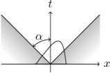
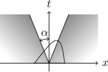
Figure 1: Illustration of the exponential growth indices. The initial data, depicted by the curve, is localized around the origin.

Theorem 2.10 (Exponential growth indices).

The following bounds hold:

1. If $|\rho(u)|^{2}\leq\operatorname{\mathit{L}}_{\rho}^{2}\left(\operatorname{\overline{\varsigma}}^{2}+u^{2}\right)$ with $\operatorname{\overline{\varsigma}}=0$ (which implies $\operatorname{\underline{\varsigma}}=\operatorname{\varsigma}=0$) and the initial data $\mu\in\mathcal{M}_{G}^{\operatorname{\beta}}(\mathbb{R})$ for some $\operatorname{\beta}>0$, then for all $p\geq 2$,

   $$\bar{\lambda}(p)\leq\begin{cases}\displaystyle\frac{\operatorname{\beta}\nu}{2}+\frac{z_{\lceil p\rceil_{2}}^{4}\operatorname{\mathit{L}}_{\rho}^{4}}{2\nu\operatorname{\beta}}\>,&\displaystyle\text{if}\quad 0\leq\operatorname{\beta}<\frac{z_{\lceil p\rceil_{2}}^{2}\operatorname{\mathit{L}}_{\rho}^{2}}{\nu}\>,\cr\displaystyle z_{\lceil p\rceil_{2}}^{2}\>\operatorname{\mathit{L}}_{\rho}^{2}\;,&\displaystyle\text{if}\quad\operatorname{\beta}\geq\frac{z_{\lceil p\rceil_{2}}^{2}\operatorname{\mathit{L}}_{\rho}^{2}}{\nu}\>,\end{cases}$$

   where $z_{m}$, $m\in\mathbb{N}$, $m\geq 2$, are the universal constants in the Burkholder-Davis-Gundy inequality. In particular, for $p=2$,

   $$\bar{\lambda}(2)\leq\begin{cases}\displaystyle\frac{\operatorname{\beta}\nu}{2}+\frac{\operatorname{\mathit{L}}_{\rho}^{4}}{8\nu\operatorname{\beta}}\;,&\displaystyle\text{if}\quad 0\leq\operatorname{\beta}<\frac{\operatorname{\mathit{L}}_{\rho}^{2}}{2\nu}\;,\cr\displaystyle\frac{1}{2}\operatorname{\mathit{L}}_{\rho}^{2}\;,&\displaystyle\text{if}\quad\operatorname{\beta}\geq\frac{\operatorname{\mathit{L}}_{\rho}^{2}}{2\nu}\>.\end{cases}$$ (2.27)

2. If $|\rho(u)|^{2}\geq\operatorname{\mathit{l}}_{\rho}^{2}\left(\operatorname{\underline{\varsigma}}^{2}+u^{2}\right)$ with $\operatorname{\underline{\varsigma}}=0$, then

   $$\underline{\lambda}(p)\geq\frac{\operatorname{\mathit{l}}_{\rho}^{2}}{2},\qquad\text{for all $\mu\in\mathcal{M}_{+}(\mathbb{R})$, $\mu\neq 0$ and all $p\geq 2$}\>;$$

   otherwise, if $\operatorname{\underline{\varsigma}}\neq 0$, then

   $$\underline{\lambda}(p)=\overline{\lambda}(p)=+\infty,\qquad\text{for all $\mu\in\mathcal{M}_{+}(\mathbb{R})$ and $p\geq 2$}\>;$$

3. In particular, for the quasi-linear case $|\rho(u)|^{2}=\lambda^{2}\left(\operatorname{\varsigma}^{2}+u^{2}\right)$ with $\lambda\neq 0$, if $\operatorname{\varsigma}=0$ and $\operatorname{\beta}\geq\frac{\lambda^{2}}{2\nu}$, then

   $$\underline{\lambda}(2)=\bar{\lambda}(2)=\lambda^{2}/2,\qquad\text{for all $\mu\in\mathcal{M}_{G,+}^{\operatorname{\beta}}(\mathbb{R})$, $\mu\neq 0$}\>;$$

   otherwise, if $\operatorname{\varsigma}\neq 0$, then

   $$\underline{\lambda}(p)=\overline{\lambda}(p)=+\infty,\qquad\text{for all $\mu\in\mathcal{M}_{+}(\mathbb{R})$ and $p\geq 2$}\;.$$

This theorem generalizes the results by Conus and Khoshnevisan [4] in several aspects: (i) more general initial data are allowed; (ii) both non trivial upper bound and lower bounds are given (compare with Theorem 1.1 [4]) for the Laplace operator case; (iii) for the parabolic Anderson model, the exact transition is proved (see Theorem 1.3 and the first open problem in [4]) for $n=2$ and the Laplace operator case; (iv) our discussions above cover the case $\rho(0)\neq 0$.

Example 2.11 (Dirac delta initial data).

Suppose that $\operatorname{\overline{\varsigma}}=\operatorname{\underline{\varsigma}}=0$. Clearly, $\delta_{0}\in\mathcal{M}_{G,+}^{\operatorname{\beta}}(\mathbb{R})$ for all $\operatorname{\beta}\geq 0$. Hence, the above theorem implies that for all even integers $k\geq 2$,

$$\frac{\operatorname{\mathit{l}}_{\rho}^{2}}{2}\leq\underline{\lambda}(k)\leq\overline{\lambda}(k)\leq z_{k}^{2}\operatorname{\mathit{L}}_{\rho}^{2}\;.$$

This recovers the previous calculation in Example 2.8.

Proposition 2.12.

Consider the parabolic Anderson model $\rho(u)=\lambda u$, $\lambda\neq 0$ with the initial data $\mu(\mathrm{d}x)=e^{-\operatorname{\beta}|x|}\mathrm{d}x$ ($\operatorname{\beta}>0$). Then we have

$$\underline{\lambda}(2)=\overline{\lambda}(2)=\begin{cases}\displaystyle\frac{\operatorname{\beta}\nu}{2}+\frac{\lambda^{4}}{8\operatorname{\beta}\nu}&\text{if $\;\;\displaystyle 0<\operatorname{\beta}\leq\frac{\lambda^{2}}{2\>\nu}$}\;,\cr\cr\displaystyle\frac{\lambda^{2}}{2}&\text{if $\;\;\displaystyle\operatorname{\beta}\geq\frac{\lambda^{2}}{2\>\nu}$}\;.\end{cases}$$

This proposition shows that for all $\operatorname{\beta}\in\left]0,+\infty\right]$, the exact phase transition occurs, and hence our upper bounds (2.27) in Theorem 2.10 for the upper growth index $\overline{\lambda}(2)$ are sharp.

2.4 Sample Path Regularity

Theorem 2.13.

Suppose that $\rho$ is Lipschitz continuous. Then the solution $u(t,x)=J_{0}(t,x)+I(t,x)$ to (1.1) has the following sample path regularity:

1. If the initial data $\mu$ is an $\alpha$-Hölder continuous function ($\alpha\in\;]0,1]$) over $\mathbb{R}$ satisfying (1.4), then

   $$J_{0}\in C_{\frac{1}{2},\alpha}\left(\mathbb{R}_{+}\times\mathbb{R}\right)\;\cup\;C_{\frac{1}{2},1}\left(\mathbb{R}_{+}^{*}\times\mathbb{R}\right)\;,\quad\text{and}\quad I\in C_{\frac{1}{4}-,\frac{1}{2}-}\left(\mathbb{R}_{+}\times\mathbb{R}\right),\quad\text{a.s.}$$

   Therefore,

   $$u=J_{0}+I\in C_{\frac{1}{4}-,\left(\frac{1}{2}-\right)\wedge\alpha}\left(\mathbb{R}_{+}\times\mathbb{R}\right)\;\cup\;C_{\frac{1}{4}-,\frac{1}{2}-}\left(\mathbb{R}_{+}^{*}\times\mathbb{R}\right),\quad\text{a.s.}$$

2. If the initial data $\mu$ is a continuous function satisfying (1.4), then

   $$J_{0}\in C_{\frac{1}{2},1}\left(\mathbb{R}_{+}^{*}\times\mathbb{R}\right)\;,\quad\text{and}\quad I\in C_{\frac{1}{4}-,\frac{1}{2}-}\left(\mathbb{R}_{+}\times\mathbb{R}\right),\quad\text{a.s.}$$

   Therefore,

   $$u=J_{0}+I\in C_{\frac{1}{4}-,\frac{1}{2}-}\left(\mathbb{R}_{+}^{*}\times\mathbb{R}\right),\quad\text{a.s.}$$

3. If the initial data $\mu$ is a signed Borel measure satisfying (1.4), then

   $$J_{0}\in C_{\frac{1}{2},1}\left(\mathbb{R}_{+}^{*}\times\mathbb{R}\right)\;,\quad\text{and}\quad I\in C_{\frac{1}{4}-,\frac{1}{2}-}\left(\mathbb{R}_{+}^{*}\times\mathbb{R}\right),\quad\text{a.s.}$$

   Therefore,

   $$u=J_{0}+I\in C_{\frac{1}{4}-,\frac{1}{2}-}\left(\mathbb{R}_{+}^{*}\times\mathbb{R}\right),\quad\text{a.s.}$$

Example 2.14 (Dirac delta initial data).

Suppose $\rho(u)=\lambda u$ with $\lambda\neq 0$. If $\mu=\delta_{0}$, then neither $J_{0}(0,x)$ nor $\lim_{t\rightarrow 0_{+}}\left|\left|I(t,x)\right|\right|_{2}$ is continuous in $x$. For $J_{0}(0,x)=\delta_{0}(x)$, this is clear. As for $\lim_{t\rightarrow 0_{+}}\left|\left|I(t,x)\right|\right|_{2}$, by Corollary 2.6 (with $\operatorname{\varsigma}=0$), we have

$$\left|\left|I(t,x)\right|\right|_{2}^{2}=\frac{1}{\lambda^{2}}\mathcal{K}(t,x)-G_{\nu}^{2}(t,x)=\frac{\lambda^{2}}{2\nu}e^{\frac{\lambda^{4}t}{4\nu}}\Phi\left(\lambda^{2}\sqrt{\frac{t}{2\nu}}\right)G_{\nu/2}(t,x)\;.$$

Therefore,

$$\lim_{t\rightarrow 0_{+}}\left|\left|I(t,x)\right|\right|_{2}^{2}=\begin{cases}0&\text{if $x\neq 0$}\;,\cr+\infty&\text{if $x=0$}\;.\end{cases}$$

References

- [1] L. Bertini and N. Cancrini. The stochastic heat equation: Feynman-Kac formula and intermittence. Journal of Statistical Physics, 78(5-6):1377–1401, 1994.
- [2] R. A. Carmona and S. A. Molchanov. Parabolic Anderson Problem and Intermittency. Mem. Amer. Math. Soc., 1994.
- [3] D. Conus, M. Joseph, D. Khoshnevisan, and S.-Y. Shiu. Initial measures for the stochastic heat equation. Annales Instit. Henri Poincaré, 2012.
- [4] D. Conus and D. Khoshnevisan. On the existence and position of the farthest peaks of a family of stochastic heat and wave equations. Probability Theory and Related Fields, 2010.
- [5] D. Conus and D. Khoshnevisan. Weak nonmild solutions to some SPDEs. Illinois Journal of Mathematics, 2010.
- [6] R. C. Dalang, D. Khoshnevisan, C. Mueller, D. Nualart, Y. Xiao, and F. Rassoul-Agha. A Minicourse on Stochastic Partial Differential Equations. Springer-Verlag, 2008.
- [7] R. C. Dalang, D. Khoshnevisan, and E. Nualart. Hitting probabilities for systems of non-linear stochastic heat equations with additive noise. ALEA Lat. Am. J. Probab. Math. Stat., 3:231–271, 2007.
- [8] R. C. Dalang, D. Khoshnevisan, and E. Nualart. Hitting probabilities for systems for non-linear stochastic heat equations with multiplicative noise. Probab. Theory Related Fields, 144(3-4):371–427, 2009.
- [9] M. Foondun and D. Khoshnevisan. Intermittence and nonlinear parabolic stochastic partial differential equations. Electr. J. Probab., 14(14):548–568, 2009.
- [10] C. Mueller. On the support of solutions to the heat equation with noise. Stochastics and Stochastics Reports, 37:225–245, 1991.
- [11] J. Pospíšil and R. Tribe. Parameter estimates and exact variations for stochastic heat equations driven by space-time white noise. Stoch. Anal. Appl., 25(3):593–611, 2007.
- [12] M. Sanz-Solé and M. Sarrà. Path properties of a class of Gaussian processes with applications to spde’s. In Stochastic processes, physics and geometry: new interplays, I (Leipzig, 1999), volume 28 of CMS Conf. Proc., pages 303–316. Amer. Math. Soc., Providence, RI, 2000.
- [13] M. Sanz-Solé and M. Sarrà. Hölder continuity for the stochastic heat equation with spatially correlated noise. In Seminar on Stochastic Analysis, Random Fields and Applications, III (Ascona, 1999), volume 52 of Progr. Probab., pages 259–268. Birkhäuser, Basel, 2002.
- [14] T. Shiga. Two contrasting properties of solutions for one-dimensional stochastic partial differential equations. Canad. J. Math., 46(2):415–437, 1994.
- [15] J. B. Walsh. An Introduction to Stochastic Partial Differential Equations. Lecture Notes in Math. 1180, 256-439, Springer, Berlin, 1986.
- [16] Y. B. Zeldovich, A. A. Ruzmaĭkin, and D. D. Sokoloff. The Almighty Chance, volume 20 of World Scientific Lecture Notes in Physics. World Scientific Publishing Co. Inc., River Edge, NJ, 1990. Translated from the Russian by Anvar Shukurov.