Primary $\gamma$-ray spectra in ⁴⁴Ti of astrophysical interest

Abstract

Primary $\gamma$-ray spectra for a wide excitation-energy range have been extracted for ⁴⁴Ti from particle-$\gamma$ coincidence data of the ⁴⁶Ti($p,t\gamma$)⁴⁴Ti reaction. These spectra reveal information on the $\gamma$-decay pattern of the nucleus, and may be used to extract the level density and radiative strength function applying the Oslo method.

Models of the level density and radiative strength function are used as input for cross-section calculations of the ⁴⁰Ca($\alpha,\gamma$)⁴⁴Ti reaction. Acceptable models should reproduce data on the ⁴⁰Ca($\alpha,\gamma$)⁴⁴Ti reaction cross section as well as the measured primary $\gamma$-ray spectra. This is only achieved when a coherent normalization of the slope of the level density and radiative strength function is performed. Thus, the overall shape of the experimental primary $\gamma$-ray spectra puts a constraint on the input models for the rate calculations.

I Introduction

The titanium isotope ⁴⁴Ti is of great astrophysical interest, since it is believed to be produced in the inner regions of core-collapse supernovae and in the normal freeze-out of Si burning layers of thermonuclear supernovae vockenhuber07 , with a large variation of yields depending on their type renaud06 . The determination of the ⁴⁴Ti yield might reveal information on the complex explosion conditions. The production yield of ⁴⁴Ti directly determines the abundance of the stable ⁴⁴Ca, and also influences the ⁴⁸Ti abundance through the feeding of ⁴⁸Cr on the $\alpha$ chain. The theoretical prediction of the ⁴⁴Ti production in core-collapse supernovae is sensitive to the chosen reaction network and the adopted nuclear reaction rates.

Cassiopeia A (Cas A) is the youngest known Galactic supernova remnant and is, at present, the only one from which $\gamma$-rays from the ⁴⁴Ti decay chain (⁴⁴Ti $\rightarrow$ ⁴⁴Sc $\rightarrow$ ⁴⁴Ca) have been unambiguously detected renaud06 . The discovery of the 1157-keV $\gamma$-ray line from ⁴⁴Ca was reported by Iyudin et al. iyudin , while measurements of the 67.9-keV and 78.4-keV lines from ⁴⁴Sc were presented by Renaud et al. renaud06 . From the combined $\gamma$-ray flux, the half-life of ⁴⁴Ti, and the distance and age of the remnant, an initial synthesized ⁴⁴Ti mass of 1.6${}^{+0.6}_{-0.3}\times 10^{-4}$ $M_{\astrosun}$ was deduced. This is thought to be unusually large, a factor of $2-10$ more than what is typically obtained by current models (see, e.g., woosley95 ; thiele96 ).

The main production reaction of ⁴⁴Ti is the ⁴⁰Ca($\alpha,\gamma$)⁴⁴Ti reaction channel with a $Q$-value of 5.127 MeV; the cross section for this reaction is very important to estimate the ⁴⁴Ti yield. Recent cross-section measurements on this reaction Nassar06 have lead to an increase of the associated astrophysical rate, giving a factor of $\sim 2$ more in the predicted yield of ⁴⁴Ti. Thus, the theoretical models become more compatible with the Cas A data; however, this would make the problem of ”young, missing, and hidden” Galactic supernova remnants even more serious: supernovae that should have occured after Cas A are still not detected by means of $\gamma$-ray emission from the ⁴⁴Ti decay chain. It is still an open question whether the Cas A is a peculiar case (asymmetric and/or a relatively more energetic explosion), or that the Cas A yield is in fact ”normal”, since it is in better agreement with the solar ⁴⁴Ca/⁵⁶Fe ratio renaud06 .

There are many uncertainties connected to the yield estimate, the most severe ones being due to astrophysical issues. However, there is also significant uncertainties related to the nuclear physics input, in particular the nuclear level density (NLD), the radiative strength function (RSF) and the $\alpha$-particle optical model potential. All these quantities are entering the calculation of the astrophysical reaction rates. The NLD is defined as the number of nuclear energy levels per energy unit at a specific excitation energy, while the RSF gives a measure of the average (reduced) transition probability for a given $\gamma$-ray energy. Both quantities are related to the average decay probability for an ensemble of levels, and are indispensable in a variety of applications (reaction rate calculations relevant for astrophysics or transmutation of nuclear waste) as well as for studying various nuclear properties in the quasicontinuum region.

In this work, we have extracted primary $\gamma$-ray spectra from the decay cascades in ⁴⁴Ti populated via the two-neutron pick-up reaction ⁴⁶Ti($p,t\gamma$)⁴⁴Ti. These spectra are measured for a wide range of initial excitation energies below the neutron threshold, and they put a constraint on the functional form of the NLD and RSF.

In Sec. II we will describe the experimental details, give an overview of the analysis, and present the obtained primary $\gamma$-ray spectra. Different normalizations of the NLD and RSF are discussed in Sec. III, and the applied models are tested against the primary $\gamma$-ray spectra in Sec. IV. In Sec. V various input models are used for estimating the ⁴⁰Ca($\alpha,\gamma$)⁴⁴Ti cross-section and reaction rates, and the calculated results are compared to existing data from Nassar et al. Nassar06 and Vockenhuber et al. vockenhuber07 . Finally, a summary and concluding remarks are given in Sec. VI.

II Experiment and analysis

The experiment was conducted at the Oslo Cyclotron Laboratory (OCL), where the Scanditronix cyclotron delivered a 32–MeV proton beam bombarding a self-supporting target of ⁴⁶Ti with mass thickness 3.0 mg/cm². The beam current was $\approx 0.5$ nA and the experiment was run for ten days. Unfortunately, the target was enriched only to 86.0% in ⁴⁶Ti. The main impurities were ⁴⁸Ti (10.6%), ⁴⁷Ti (1.6%), ⁵⁰Ti (1.0%), and ⁴⁹Ti (0.8%). The reaction of interest, ⁴⁶Ti($p,t\gamma$)⁴⁴Ti, has a $Q$-value of $-14.236$ MeV qcalc . Particle-$\gamma$ coincidences from this reaction were measured with eight collimated Si $\Delta E-E$ particle detectors and the CACTUS multidetector system CACTUS .

The Si detectors were placed in a circle in forward direction, $45^{\circ}$ relative to the beam axis. The front ($\Delta E$) and end ($E$) detectors had a thickness of $\approx 140$ $\mu$m and $1500$ $\mu$m, respectively. The CACTUS array consists of 28 collimated $5"\times 5"$ NaI(Tl) crystals for detecting $\gamma$-rays. The total efficiency of CACTUS is $15.2(1)$% at $E_{\gamma}=1332.5$ keV. Also a Ge detector was placed in the CACTUS frame to monitor the experiment. The charged ejectiles and the $\gamma$-rays were measured in coincidence event-by-event.

To identify the charged ejectiles of the reactions, the well-known $\Delta E-E$ technique is used. In Fig. 1, the energy deposited in the $\Delta E$ detector versus the energy deposited in the $E$ detector is shown for one particle telescope. Each ”banana” in the figure corresponds to a specific particle species as indicated in the figure.

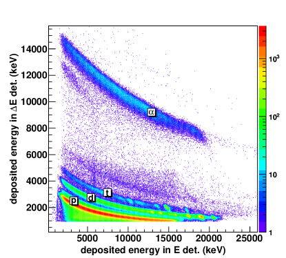
Figure 1: (Color online). Identification of particle species using the $\Delta E-E$ technique.

By gating on the triton ”banana”, the events with the reaction ⁴⁶Ti($p,t\gamma$)⁴⁴Ti were isolated. The ⁴⁶Ti($p,d\gamma$)⁴⁵Ti data have been published previously in Ref. Naeem_45Ti . The singles and coincidence triton spectra are shown in Fig. 2. We note that the excited 1.904-MeV 0⁺ state ($E_{t}\approx 16$ MeV) is rather weakly populated. This is expected on the basis that $\ell=0$ states are in general much weaker populated in the ($p,t$) reaction at $45^{\circ}$ compared to, e.g., $\ell=2$ and 4, see Ref. rapaport . The populated spin range is estimated to $J\approx 0-6\hbar$ based on the observed triton peaks and their coincident $\gamma$-decay cascades, in accordance with the findings in Ref. rapaport .

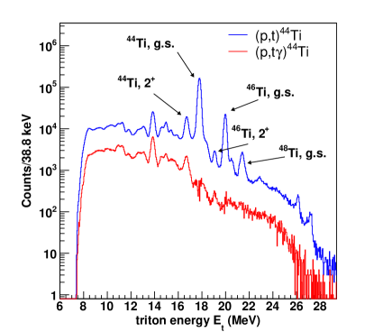
Figure 2: (Color online). Singles (blue) and coincidence (red) triton spectra. The impurities of ^48,50Ti are easily seen. The resolution is $\approx 270-330$ keV.

Two-neutron pick-up on the ^48,50Ti impurities in the target give rise to peaks at higher triton energies than the ground state of ⁴⁴Ti due to their lower reaction thresholds; the $Q$-values are $-12.025$ and $-10.560$ MeV for the ⁴⁴Ti($p,t\gamma$)⁴⁶Ti and ⁵⁰Ti($p,t\gamma$)⁴⁸Ti reactions, respectively. This means that there is a background from such events in the spectra that cannot be removed (an $\approx 14$% effect).

Using reaction kinematics and the known $Q$-value for the reaction, the measured triton energy was transformed into excitation energy of the residual nucleus. Thus, the $\gamma$-ray spectra are tagged with a specific initial excitation energy in ⁴⁴Ti. Further, the $\gamma$-ray spectra were corrected for the known response functions of the CACTUS array following the procedure described in Ref. gutt6 . The main advantage of this correction method is that the experimental statistical uncertainties are preserved, without introducing any new, artificial fluctuations.

Information on NLD and RSF can be extracted from the distribution of primary $\gamma$-rays, that is, the $\gamma$-rays that are emitted first in each decay cascade. To separate these first-generation $\gamma$ transitions from the second and higher-order generations, an iterative subtraction technique is used Gut87 . The $\gamma$-ray spectra $f_{i}$ for excitation-energy bin $i$ obviously contain all generations of $\gamma$-rays from all possible cascades decaying from the excited states of this bin. The subtraction technique is based on the assumption that the spectra $f_{j<i}$ for all the energy bins $E_{j}<E_{i}$ contain the same $\gamma$-transitions as $f_{i}$ except the first $\gamma$-rays emitted, since they will bring the nucleus from the states in bin $i$ to underlying states in the energy bins $j$. This is true if the main assumption of this technique holds: that the decay routes are the same whether they were initiated directly by the nuclear reaction or by $\gamma$ decay from higher-lying states.

The obtained first-generation matrix $P(E,E_{\gamma})$ of ⁴⁴Ti is shown in Fig. 3.

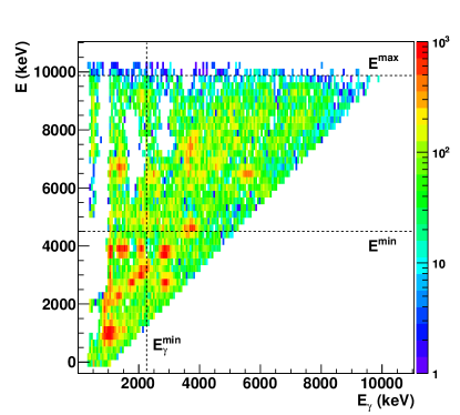
Figure 3: (Color online). The first-generation spectra for each excitation-energy bin in ⁴⁴Ti. The dashed lines are limits set for the further analysis (see text).

The diagonal where $E=E_{\gamma}$ is clearly seen. Here, two peaks are particularly pronounced: one from the decay of the first excited state at $E=E_{\gamma}=1083$ keV, and the other from the decay of the second $2^{+}$ state at $2887$ keV to the ground state. There are also more diagonals visible, e.g., for $E_{\gamma}=E-1083$ keV where the decay goes directly to the first excited $2^{+}$ state, and so on.

Before extracting the NLD and RSF from the $P$ matrix, we have set a lower limit for the $\gamma$-ray energies ($E_{\gamma}^{\mathrm{min}}$), and a lower and upper limit for the excitation energy ($E_{\mathrm{min}}$, $E_{\mathrm{max}})$. The limits on the excitation-energy side are put to ensure that the spectra are dominated by decay from compound states ($E_{\mathrm{min}}$), and that the statistics is not too low ($E_{\mathrm{max}}$). On the $\gamma$-ray energy side the limit is set to exclude possible left-overs of higher-generation decay, that might not be correctly subtracted in the first-generation method (see Refs. systematic ; Schiller00 and references therein for more details). In Fig. 4, the original, unfolded, and first-generation $\gamma$-ray spectrum of ⁴⁴Ti for excitation energy $E=6.1$ MeV are displayed.

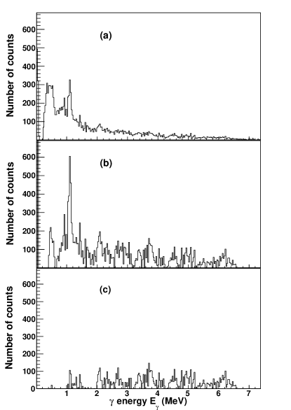
Figure 4: Original (a), unfolded (b) and first-generation (c) $\gamma$-ray spectrum of ⁴⁴Ti for excitation energy $E=6.1$ MeV.

With the first-generation matrix properly prepared, an iterative procedure is applied to extract NLD and RSF from the primary $\gamma$-ray spectra. The method is based on the assumption that the reaction leaves the product nucleus in a compound state, which then subsequently decays in a manner that is independent on the way it was formed, i.e. a statistical decay process BM . This is a reasonable assumption for states in the quasicontinuum, where the typical lifetime of the states is of the order of $10^{-15}$ $s$, whereas the reaction time is $\approx 10^{-18}$ $s$. In addition, the configuration mixing of the levels is expected to be significant if the level spacing is comparable to the residual interaction BM . This is normally fulfilled in the region of high level density.

If compound states are indeed populated, the $\gamma$ decay from these states should be independent of the reaction used to reach them. In previous works (e.g. Ref. Mo_nld ) it has been demonstrated that the direct reactions (³He,³He^′) and (³He,$\alpha$) into the same final nucleus do produce very similar decay cascades. Also, the extracted NLD and RSF was found to be equal within the expected fluctuations This indicates that even though a direct reaction such as ($p,t$) is used, compound states are likely to be populated at sufficiently high excitation energy (as mentioned already for the $E_{\mathrm{min}}$ limit set in the first-generation matrix $P(E,E_{\gamma})$).

The ansatz for the iterative method is Schiller00 :

$$P(E,E_{\gamma})\propto\rho(E_{\mathrm{f}}){\mathcal{T}}(E_{\gamma}),$$ (1)

meaning that the first-generation matrix $P(E,E_{\gamma})$ is assumed to be separable into two vectors that give directly the functional form of the level density at the final excitation energy $E_{\mathrm{f}}=E-E_{\gamma}$, and the $\gamma$-ray transmission coefficient $\cal{T}$ for a given $E_{\gamma}$. This is done by minimizing

$$\chi^{2}=\frac{1}{N_{\mathrm{free}}}\sum_{E=E^{\mathrm{min}}}^{E^{\mathrm{max}}}\sum_{E_{\gamma}=E_{\gamma}^{\mathrm{min}}}^{E}\left(\frac{P_{\mathrm{th}}(E,E_{\gamma})-P(E,E_{\gamma})}{\Delta P(E,E_{\gamma})}\right)^{2},$$ (2)

where $N_{\mathrm{free}}$ is the number of degrees of freedom, $\Delta P(E,E_{\gamma})$ is the uncertainty in the experimental first-generation $\gamma$-ray matrix $P(E,E_{\gamma})$, and the theoretical first-generation matrix is given by

$$P_{\mathrm{th}}(E,E_{\gamma})=\frac{\rho(E-E_{\gamma}){\mathcal{T}}(E_{\gamma})}{\sum_{E_{\gamma}=E_{\gamma}^{\mathrm{min}}}^{E}\rho(E-E_{\gamma}){\mathcal{T}}(E_{\gamma})}.$$ (3)

Every point of the $\rho$ and ${\mathcal{T}}$ functions is assumed to be an independent variable, so that the reduced $\chi^{2}$ of Eq. (2) is minimized for every argument $E-E_{\gamma}$ and $E_{\gamma}$. Note that $\cal{T}$ is independent of excitation energy according to the Brink hypothesis brink . If we had an excitation-energy dependent $\gamma$-ray transmission coefficient, ${\cal T}={\cal T}(E,E_{\gamma})$, it would in principle be impossible to disentangle the level density and the $\gamma$-ray transmission coefficient.

It is well known that the Brink hypothesis is violated when high temperatures and/or spins are involved in the nuclear reactions, as shown for giant dipole resonance (GDR) excitations in Ref. Andreas&Thoennessen and references therein. However, since both the temperature reached ($T\propto\sqrt{E_{\mathrm{f}}}$) and the spins populated ($J\sim 0-6\hbar$) are rather low for the experiment in this work, these dependencies are assumed to be of minor importance in the excitation-energy region of interest here.

To inspect how well the iterative procedure works, we have compared the experimental first-generation spectra for several excitation energies with the ones obtained by multiplying the extracted $\rho$ and $\cal{T}$ functions. The result for a selection of primary $\gamma$-ray spectra is shown in Fig. 5.

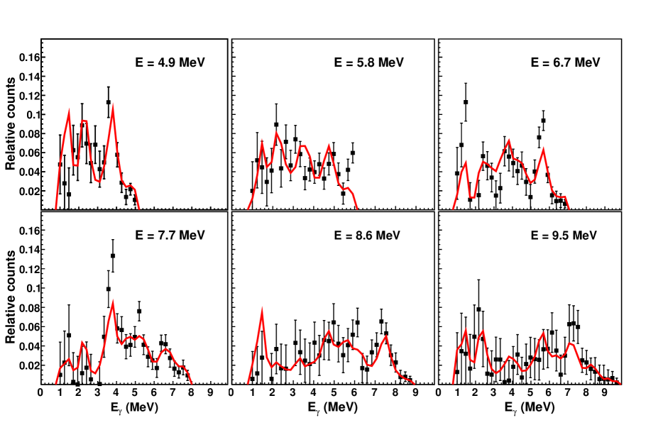
Figure 5: (Color online). Comparison of experimental primary $\gamma$-ray spectra (filled squares) and the ones obtained from multiplying the extracted $\rho$ and $\cal{T}$ functions (red line) for several excitation energies. The experimental and calculated spectra are shown for excitation-energy bins of 467 keV.

As can be seen, the agreement between the calculated and the experimental first-generation spectra are in general quite good, although there are local variations where the calculated spectra are not within the error bars of the experimental ones. These variations could well be due to large Porter-Thomas fluctuations PT , as there are relatively few levels in this nucleus.

The iterative procedure to obtain the level density and the $\gamma$-ray transmission coefficient uniquely determines the functional form of $\rho$ and $\cal{T}$; however, identical fits to the experimental data is achieved with the transformations Schiller00

$$\tilde{\rho}(E-E_{\gamma}) = A\exp[\alpha(E-E_{\gamma})]\,\rho(E-E_{\gamma}),$$ (4)

$$\tilde{{\mathcal{T}}}(E_{\gamma}) = B\exp(\alpha E_{\gamma}){\mathcal{T}}(E_{\gamma}).$$ (5)

Thus, to obtain the absolute normalization of the level density and $\gamma$-ray transmission coefficient, the transformation parameters $A$, $\alpha$, and $B$ must be determined independently.

III Normalizations and models for
level density and radiative strength function

III.1 Level density

Usually, the level density $\rho(E_{f})$ is normalized to known, discrete levels at low excitation energy, and to the total level density at the neutron separation energy $\rho(S_{n})$, which is deduced from neutron resonance spacings $D_{0}$ and/or $D_{1}$ (see, e.g., Ref. Pb ). However, for the ⁴⁴Ti case, no neutron (or proton) resonance data are known since the target nuclei for the neutron and proton capture reactions are unstable. We are therefore left with only two types of experimental constraints, namely the known levels at low excitation energy and the observed first-generation spectra (which also depend on the $\gamma$-ray strength).

We have chosen two different approaches to normalize our data, and, out of those, to estimate the sensitivity on our results to this normalization procedure: (i) apply theoretical level densities based on microscopic calculations, and (ii) use a standard closed-form formula with global parameters. For the first approach, we have used recent calculations of Goriely, Hilaire and Koning go08 (hereafter labeled GHK). For the second approach, we have applied the constant-temperature (CT) formula GC :

$$\rho_{\mathrm{CT}}(E)=\frac{1}{T}\exp{\left(\frac{E-E_{0}}{T}\right)},$$ (6)

where the nuclear temperature $T=1.50$ MeV and the energy shift $E_{0}=-0.08$ MeV are taken from the global parameterization of Refs. koning08 ; TALYS . The level-density data normalized to these two approaches are shown in Fig. 6.

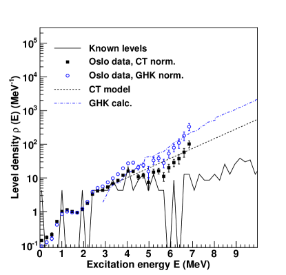
Figure 6: (Color online) Experimental data points (filled squares) normalized to the CT model (dashed line) and data points (blue, open circles) normalized to the calculation of GHK (dashed-dotted line). The black, solid line represents the known levels taken from Ref. ENSDF .

We observe that our data follow closely the known, discrete levels ENSDF at low excitation energy, and especially in the region $2.4<E<5.2$ MeV. This is gratifying, as it implies that the Oslo method does indeed give reasonable results for the level density. We also see that there is a decrease in the level density for $4.0<E<5.2$ MeV and an abrupt increase for $5.8<E<6.2$ MeV. These structures are not well described by any of the models used for normalization. They might be due to shell effects and/or $\alpha$-clustering effects (since ⁴⁴Ti is an $N=Z$ nucleus). An increase in the level density could also indicate the breaking of a nucleon Cooper pair and/or the crossing of a shell gap.

We note that both the ground state and the 0⁺ state at $E=1.9$ MeV are not very pronounced in Fig. 6. Also, we see that there is less direct decay to the ground state and the excited 0⁺ state compared to the 2⁺ state at 1083 keV and the 4⁺ state at 2454 keV, especially at higher excitation energies (see Fig. 3). This could imply that there are relatively few spin-1 states populated in the ($p,t$) reaction (assuming that dipole radiation is dominant in this region). This is not surprising because the spin distribution is expected to have a maximum for $J=3-4$.

We see that the resolution on the level density is rather poor at low excitation energies, roughly 600 keV for the first excited 2⁺ state. This may be explained by the fact that the level density in this region is mainly determined by decay involving high-energy $\gamma$ rays, which have a resolution of up to $\approx 300$ keV (similar to the triton-energy resolution). As a consequence, the resolution of the level density gets better and better for increasing excitation energy. In addition, the rather large amount of other Ti isotopes in the target may give a smoothing effect on the extracted quantities (both the NLD and RSF).

III.2 Radiative strength function

Because there are no experimental data on neither the level spacing $D$ nor the total, average radiative width for s-wave resonances $\left<\Gamma_{\gamma 0}\right>$ for ⁴⁴Ti, we must find the absolute normalization parameter $B$ of the RSF by other means. In order to have a rough approximation of the absolute strength, we have looked at experimental values of $\left<\Gamma_{\gamma 0}\right>$ for other Ti isotopes found in Ref. RIPL2 , see Fig. 7. From these values, the educated guess of $\left<\Gamma_{\gamma 0}\right>=1200(600)$ meV seems to be reasonable for ⁴⁴Ti. The RSFs of ⁴⁴Ti for the two choices of level-density normalization are shown in Fig. 8. Also the upper and lower limits are indicated, corresponding to $\left<\Gamma_{\gamma 0}\right>=1800$ meV for the CT normalization and $\left<\Gamma_{\gamma 0}\right>=600$ meV for the GHK normalization, respectively.

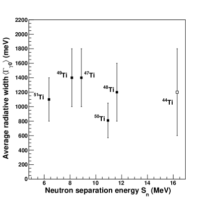
Figure 7: Experimental average radiative width (filled squares) for ^47-51Ti as a function of neutron separation energy, and estimated width for ⁴⁴Ti (open square).

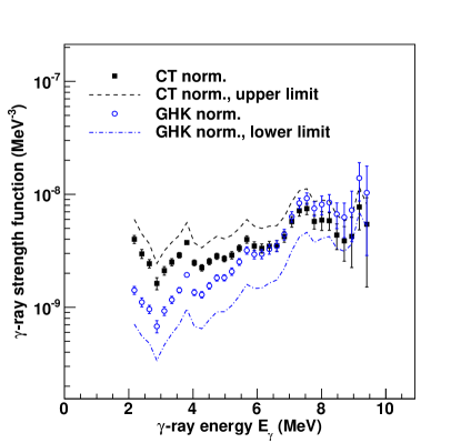
Figure 8: (Color online). Normalized radiative strength functions for the two normalizations of the level density. The dashed line is the upper limit for the CT normalization, while the dashed-dotted line is the lower limit for the GHK normalization.

From Fig. 8, it is seen that for $E_{\gamma}>4$ MeV, the RSF of ⁴⁴Ti seems to reach a relatively smooth behavior with increasing strength as a function of $E_{\gamma}$. Naturally, as seen from Eq. 5, the slope varies depending on the normalization chosen for the level density. For energies below $E_{\gamma}\approx 4$ MeV, we observe on average a slight increase in strength for decreasing $\gamma$-ray energy. However, we see that the data in this region display quite large variations, which could be due to Porter-Thomas fluctuations PT .

A low-energy increase in the RSF data has been seen previously in several light and medium-mass nuclei with the Oslo method Fe_Alex ; Fe_Emel ; Mo_RSF ; V ; Sc , with the two-step cascade method following neutron capture Fe_Alex , and recently also in proton capture Ni_Alex . However, for ⁴⁴Ti, the increase at low energies is not as strong as in, e.g., ^56,57Fe Fe_Alex .

As of today, it is not clear whether the low-energy increase is due to some sort of collective decay mode(s) or if it is an effect of other structural effects in these nuclei. An analysis of simulated data using the DICEBOX code DICEBOX has demonstrated that for light nuclei, the spin distribution of the initial populated levels may have a considerable influence on the possible decay paths from these levels systematic . This seems to be due to a combination of several factors: (i) the low level density in light nuclei at low excitation energy, (ii) restrictions on the possible populated spins of the initial levels, (iii) the dominance of dipole radiation from highly excited levels, and (iv) a rather large asymmetric parity distribution up to rather high excitation energies. As is shown in Ref. systematic , these factors may lead to a significant increase in the extracted RSF for low $\gamma$-ray energies compared to the input RSF function used to generate the $\gamma$-ray spectra. It is not unlikely that a similar effect may be present in ⁴⁴Ti as well.

III.3 Models for the radiative strength function

In general, the $\gamma$ decay in quasicontinuum is expected to be dominated by electric dipole radiations. Also, there is experimental evidence that a giant magnetic dipole resonance (also known as the magnetic spin-flip resonance) is present in several light and medium-mass nuclei (see, e.g., Ref. Djalali ).

We have applied the commonly used Generalized Lorentzian (GLO) expression ko87 ; ko90 for the $E1$ strength. This model is given by ko90

$$f_{\rm GLO}(E_{\gamma},T_{f})=\frac{1}{3\pi^{2}\hbar^{2}c^{2}}\sigma_{E1}\Gamma_{E1}\times$$ (7)

$$\left[\frac{E_{\gamma}\Gamma(E_{\gamma},T_{f})}{(E_{\gamma}^{2}-E_{E1}^{2})^{2}+E_{\gamma}^{2}\Gamma(E_{\gamma},T_{f})^{2}}+\;0.7\frac{\Gamma(E_{\gamma}=0,T_{f})}{E_{E1}^{3}}\right],$$

where the Lorentzian parameters $\Gamma_{E1}$, $E_{E1}$ and $\sigma_{E1}$ correspond to the width, centroid energy, and peak cross section of the giant electric dipole resonance (GDR). We have made use of the parameterization of RIPL-2 RIPL2 to estimate the GDR parameters as these are unknown experimentally. Due to the dynamic ground-state deformation of ⁴⁴Ti ($\beta_{2}=0.27$ RIPL2 ), the GDR is assumed to be split in two components and thus two sets of GDR parameters are applied (see Tab. 1). In addition, we have assumed a constant temperature $T_{f}$ of the final states in accordance with the Brink hypothesis brink .

In order to account for the small increase in strength at low energies, we have added a Lorentzian resonance of the form

$$f_{\mathrm{up}}(E_{\gamma})=\frac{1}{3\pi^{2}\hbar^{2}c^{2}}\frac{\sigma_{\mathrm{up}}E_{\gamma}\Gamma_{\mathrm{up}}^{2}}{(E_{\gamma}^{2}-E_{\mathrm{up}}^{2})^{2}+E_{\gamma}^{2}\Gamma_{\mathrm{up}}^{2}},$$ (8)

with centroid energy $E_{\mathrm{up}}=1.9$ MeV, width $\Gamma_{\mathrm{up}}=1.3$ MeV, and a peak cross section $\sigma_{\mathrm{up}}$ that will vary according to which NLD model that has been used for normalization. Such a shape of the low-energy increase seems to be in accordance with data and model descriptions in Refs. milan ; steve for the Mo nuclei, and was used also in Ref. upbend_cross . The constant temperature $T_{f}$ is slightly varied for the two models to give the best fit to the data. All parameters used are given in Tab. 1.

The lower and upper limit of the absolute normalization will necessarily give slightly different parameters to get the best fit to the data. These parameters are also given in Tab. 1.

Another frequently used model for $E1$ strength is the standard Lorentzian (the Brink-Axel model, see Ref. RIPL2 and references therein). The expression reads

$$f_{\mathrm{SLO}}(E_{\gamma})=\frac{1}{3\pi^{2}\hbar^{2}c^{2}}\frac{\sigma_{E1}E_{\gamma}\Gamma_{E1}^{2}}{(E_{\gamma}^{2}-E_{E1}^{2})^{2}+E_{\gamma}^{2}\Gamma_{E1}^{2}}.$$ (9)

This model is independent of excitation energy, in accordance with our assumption behind Eq. (1). However, as described in Ref. RIPL2 , this model is known to generally overestimate the value of $\left<\Gamma_{\gamma 0}\right>$ and neutron-capture cross sections.

For the magnetic transitions, a standard Lorentzian as recommended by the RIPL-2 library RIPL2 and shown in Fig. 9 is adopted (see Table 1 for the corresponding parameters).

Table 1: Parameters used for the RSF models.

Model	$E_{E1,1}$	$\sigma_{E1,1}$	$\Gamma_{E1,1}$	$E_{E1,2}$	$\sigma_{E1,2}$	$\Gamma_{E1,2}$	$T_{f}$	$E_{M1}$	$\sigma_{M1}$	$\Gamma_{M1}$	$E_{\mathrm{up}}$	$\sigma_{\mathrm{up}}$	$\Gamma_{\mathrm{up}}$
	(MeV)	(mb)	(MeV)	(MeV)	(mb)	(MeV)	(MeV)	(MeV)	(mb)	(MeV)	(MeV)	(mb)	(MeV)
CT+GLO	17.23	43.16	5.98	21.58	21.54	9.19	0.50	11.6	0.8	4.0	1.9	0.060	1.3
CT+GLO, upper limit	17.23	43.16	5.98	21.58	21.54	9.19	0.80	11.6	0.9	4.0	1.9	0.070	1.3
GHK+GLO	17.23	43.16	5.98	21.58	21.54	9.19	0.40	11.6	0.7	4.0	1.9	0.015	1.3
GHK+GLO, lower limit	17.23	43.16	5.98	21.58	21.54	9.19	0.15	11.6	0.3	4.0	1.9	0.010	1.3

The resulting models and the extracted data for the two adopted NLD normalizations are shown in Fig. 9 (the models corresponding to the best fit for the lower and upper normalization limits are not shown).

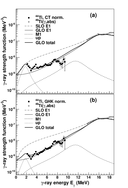
Figure 9: Radiative strength functions and fitted models for (a) the CT and (b) the GHK normalization. Note that the SLO model has not been fitted to the data.

We see from Fig. 9 that the shape of the SLO model does not fit the extracted RSF very well; in particular the low-energy part is very different in shape. The enhancement of the RSF data at low $\gamma$-ray energies may be explained by the spin distribution of the initial levels as described previously.

III.4 Temperature dependence of the strength function

As discussed already, we rely on the Brink hypothesis when extracting the NLD and RSF. We would like to investigate if this hypothesis is reasonable, and we have therefore extracted the RSF for two different excitation-energy regions, $4.5\leq E\leq 7.1$ MeV and $7.3\leq E\leq 9.9$ MeV (see Fig. 10 for the result using the CT normalization). We observe that there are rather large, local fluctuations, e.g. at $E_{\gamma}\approx 5.5$ MeV, that makes it hard to draw any firm conclusion whether the extracted RSF is dependent on excitation energy or not. As already mentioned, we expect large differences due to Porter-Thomas fluctuations in the decay strength of this nucleus. However, the gross features seem to be quite similar for the two excitation-energy ranges.

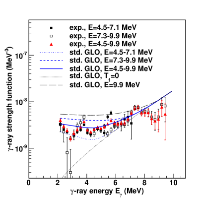
Figure 10: (Color online) Radiative strength functions extracted for two different excitation-energy regions as compared to the one from the total excitation-energy region under consideration (all cases are normalized to the CT level density). The standard GLO model is also shown for these ranges of excitation energy and the extreme cases $T_{f}=0$ and $E=9.9$ MeV.

To get a better understanding on the possible temperature dependence, we have also used the standard GLO model with a varying temperature corresponding to the accessible final excitation energies of the two ranges. The temperature is estimated by $T_{f}\propto\sqrt{E_{f}}$, and the models displayed in Fig. 10 represent the average RSF within the three excitation-energy regions $4.5\leq E\leq 7.1$ MeV, $7.3\leq E\leq 9.9$ MeV, and $4.5\leq E\leq 9.9$ MeV. The maximum final temperature reached is in the range 0.50–1.14 MeV for initial excitation energies between $4.5-9.9$ MeV and with $E_{\gamma}^{\mathrm{min}}=2.2$ MeV.

We observe that for $\gamma$ energies between $2.2-5.2$ MeV, the upper range can give more than a factor of two larger $\gamma$ strength in the GLO model than the lower range. The largest experimental fluctuations are also of the order of a factor two, but on average, the experimental data seem not to have such a strong dependence on the final excitation energy as the standard GLO model would imply.

Finally, we have calculated the GLO model for the direct decay to the ground state ($T_{f}=0$ MeV) and for the highest temperatures reached, namely for initial excitation energy $E=9.9$ MeV. These cases are also displayed in Fig. 10. It is clear that the zero-temperature calculation is not similar to the experimental data below $E_{\gamma}\approx 6$ MeV. In fact, the experimental data lie in between the two extreme cases. As argued above, the overall shape of the RSF seem to be rather similar for the two excitation-energy ranges. Thus, it is probably quite reasonable to apply a constant temperature in the GLO model in accordance with the Brink hypothesis. We note however that the GLO model averaged over the total excitation-energy range covered (blue solid line in Fig. 10) agrees rather well with the average shape of the experimental data.

IV Reproduction of experimental primary $\gamma$-ray spectra

As described in the previous section, both the NLD and RSF deduced from the present experiment are affected by severe uncertainties associated with the normalization procedure that in the case of ⁴⁴Ti cannot be reliably constrained by additional experimental data. For this reason, the different NLD and RSF models are now directly tested on the primary $\gamma$-ray spectra, which in turn correspond to the fundamental quantity entering the description of the radiative decay in reaction models.

There are 24 experimental spectra for excitation energies $4.5\leq E\leq 9.9$ MeV with bin size 233.4 keV. Due to the poor statistics, we have compared the average of two bins as in Fig. 5. For the level density, we have applied the known levels for $E<3.7$ MeV, and either the CT model or the GHK calculation above this energy. The calculated spectra are scaled to get the best possible agreement with the experimental spectra, which are normalized such that $\sum_{E_{\gamma}=E_{\gamma}^{\mathrm{min}}}^{E}P(E,E_{\gamma})=1$.

We have also calculated the primary $\gamma$ spectra using the standard GLO model with a variable temperature in combination with the two level density models. For each initial excitation energy ($4.5\leq E\leq 9.9$ MeV), we have used the GLO model with $T_{f}\propto\sqrt{E_{f}}$ and made an average of all these RSFs for the whole excitation-energy region that is used for the analysis.

Finally, we have applied the SLO model in combination with the two NLD models.

The six model combinations shown in Figs. 11–12 thus correspond to:

• input 1: the CT level density and the fitted GLO model with constant temperature.

• input 2: the GHK level density and the fitted GLO model with constant temperature.

• input 3: the CT level density and standard GLO model averaged over the experimental excitation-energy range (blue, solid line in Fig. 10).

• input 4: GHK level density and standard GLO model averaged over the experimental excitation-energy range (blue, solid line in Fig. 10).

• input 5: the CT level density and the SLO model.

• input 6: the GHK level density and the SLO model.

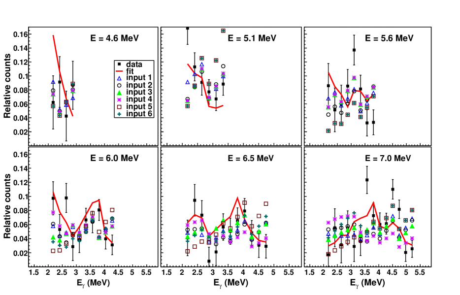
Figure 11: (Color online) Experimental primary $\gamma$ spectra (filled squares) and those obtained from multiplying the extracted $\rho$ and $\cal{T}$ functions (red line) for $4.6\leq E\leq 7.0$ MeV. These are compared with calculated spectra using the six inputs as described in the text. The experimental and calculated spectra are given for excitation-energy bins of 466.8 keV.

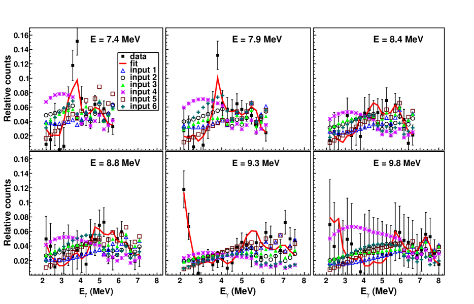
Figure 12: (Color online) Same as Fig. 11 for $7.4\leq E\leq 9.8$ MeV.

We find that for the lower excitation energies ($E\leq 7.0$ MeV), all the input models give a rather good reproduction of the spectra, and also they give relatively similar results. However, for the higher excitation energies ($7.4\leq E\leq 9.8$ MeV), there are clear deviations for the different inputs, and input 4 gives a significantly worse fit than the others. This is not so surprising, considering that the slope of the standard GLO model is very different from the RSF model fitted to our data using the GHK level density. It is seen in Fig. 12 that this mismatch in slope leads to a wrong overall shape of the primary spectra (overestimating the low-energy part and underestimating the high-energy part). The models that are consistent in slope behave much better.

In general, for the high-energy region, input 2 and input 3 give the best reproduction of the experimental spectra out of the six model combinations. The SLO model gives also rather good results, in particular in combination with the GHK level density. This could be an indication that the overall shape of this model might be correct, although the absolute value is probably too large (as seen in Fig. 9). However, in combination with the CT level density the spectra calculated with this model underestimate the intensity of the low-energy $\gamma$ rays compared to the measured ones.

Naturally, using the extracted $\rho$ and $\mathcal{T}$ data points give a much better fit than any model, as structures especially in the level density are lost when using the smooth models.

V Capture cross section and Maxwellian-averaged rate

The model combinations described in Sec. IV can further be applied for estimating the ⁴⁰Ca($\alpha,\gamma$)⁴⁴Ti cross section and the corresponding reaction rate. We have used the code TALYS TALYS for the cross-section and reaction-rate calculations. In all calculations we have used the $\alpha$ optical-model potential (OMP) of McFadden and Satchler McFadden . We have also tested other $\alpha$-OMPs such as the one developed by Demetriou, Grama and Goriely demetriou ; however, it turns out that in this case, the results are rather insensitive to the choice of $\alpha$-OMP.

The model sets applied for the cross-section and reaction-rate calculations are:

• input 1: the CT level density and the corresponding fitted GLO model.

• input 2: the GHK level density and the corresponding fitted GLO model.

• input 5: the CT level density and the SLO model.

• input 6: the GHK level density and the SLO model.

• input 7: the CT level density and the standard GLO model.

• input 8: the GHK level density and the standard GLO model.

• input 9: the CT level density and the corresponding fitted GLO model for the upper normalization limit ($\left<\Gamma_{\gamma 0}\right>=1800$ meV).

• input 10: the GHK level density and the corresponding fitted GLO model for the lower normalization limit ($\left<\Gamma_{\gamma 0}\right>=600$ meV).

For the standard GLO model, we have followed the prescription used in TALYS, where the temperature of the final states is calculated from the relation RIPL2

$$T_{f}=\sqrt{(E_{i}-\Delta-E_{\gamma})/a}.$$ (10)

Here, $E_{i}$ is the initial excitation energy in the compound nucleus, $\Delta$ is a pairing correction, and $a$ is the level density parameter. There is thus a specific GLO RSF for each initial excitation energy (no averaging over a large excitation-energy window as was done with inputs 3 and 4 in Sec. IV).

The Maxwellian-averaged astrophysical reaction rate $N_{A}\left<\sigma v\right>(T)$ for a temperature $T$ is given by

$$N_{A} \left<\sigma v\right>(T)=\left(\frac{8}{\pi m}\right)^{1/2}\frac{N_{A}}{(kT)^{3/2}G(T)}\times$$ (11)

$$\int_{0}^{\infty}\sum_{\mu}\frac{(2I^{\mu}+1)}{(2I^{0}+1)}\sigma^{\mu}(E)E\exp\left[-\frac{(E+E_{x}^{\mu})}{kT}\right]dE,$$

where $m$ is the reduced mass of the initial system of projectile (here the $\alpha$ particle) and target nucleus (here ⁴⁰Ca), $k$ is the Boltzmann constant, $N_{A}$ is Avogadro’s number, $E$ is the relative energy of the target and projectile, $I^{\mu},E_{x}^{\mu}$ are the spin and excitation energy for the excited states labeled $\mu$, and $\sigma^{\mu}$ is the reaction cross section. Further, the temperature-dependent, normalized partition function $G(T)$ reads

$$G(T)=\sum_{\mu}(2I^{\mu}+1)/(2I^{0}+1)\exp(-E_{x}^{\mu}/kT).$$ (12)

See the TALYS documentation for more details TALYS .

For the above expressions, local thermodynamic equilibrium is assumed in the astrophysical environment, so that the energies of both the targets and projectiles as well as their relative energies $E$ obey Maxwell-Boltzmann distributions corresponding to the temperature $T$ at that location. Also the relative populations of the various nuclear levels with spin and excitation energy $I^{\mu},E_{x}^{\mu}$ obey a Maxwell-Boltzmann distribution.

V.1 Uncertainties in the calculations

The key ingredients in the rate calculations (NLD, RSF, and $\alpha$-OMP) all contribute to the uncertainties but in different temperature regions. By varying the $\alpha$-OMP, the rate will change most at low temperatures (below $\approx 1.5\cdot 10^{9}$ K), while the NLD and RSF both have a significant impact on the rate at higher temperatures (above $\approx 1.5\cdot 10^{9}$ K).

The ⁴⁰Ca($\alpha,\gamma$) reaction only populates states with total isospin zero in ⁴⁴Ti, and dipole transitions with no change in total isospin are suppressed in self-conjugate $N=Z$ nuclei Holmes . Since complete isospin mixing is assumed in the determination of the RSF, a corrective factor must be included before applying the extracted RSFs in the cross section and reaction rate calculations. For $\alpha$-captures, a standard prescription is to divide the RSF by a constant factor $f_{\mathrm{iso}}$ of typically 5 to 8 Nassar06 ; Holmes , giving a reduced RSF $f^{\prime}$ of $f^{\prime}=f/f_{\mathrm{iso}}$.

However, it is not obvious how the value of this correction factor should be determined, as it is related to the degree of isospin mixing (for a large degree of mixing the correction factor should be small and vice versa). Also, high-energy $\gamma$ rays decay to low-lying states, where the isospin mixing might be small, while low-energy $\gamma$ rays decay in the quasi-continuum, where one expects a large degree of mixing. Therefore, one could in principle expect that $f_{\mathrm{iso}}$ would vary as a function of $\gamma$ energy. To estimate such a function is however a very complicated task and beyond the scope of the present work. We will therefore assume a constant $f_{\mathrm{iso}}$, although this is probably quite crude.

Another source of uncertainty is the value of $\left<\Gamma_{\gamma 0}\right>$. Since this value is not known experimentally, the uncertainty in this quantity is correlated to the uncertainty in $f_{\mathrm{iso}}$. This is because one can obtain basically the same cross section and reaction rate for a range of $\left<\Gamma_{\gamma 0}\right>$ values by adjusting $f_{\mathrm{iso}}$ correspondingly (a small value of $\left<\Gamma_{\gamma 0}\right>$ in combination with a small $f_{\mathrm{iso}}$ and vice versa).

We have calculated the integral cross section of the ($\alpha,\gamma$)⁴⁴Ti reaction for incoming $\alpha$ energies between $2.1-4.2$ MeV. This corresponds to excitation energies in ⁴⁴Ti in the range $E=7.2-9.3$ MeV, which is the most relevant region for astrophysics. In the calculations, we have adopted a constant $f_{\mathrm{iso}}=5$, and we have also tested a larger correction factor of $f_{\mathrm{iso}}=8$. In addition, we have considered the assumed uncertainty of 50% in the estimated value of $\left<\Gamma_{\gamma 0}\right>$ combined with the uncertainty in slope (either the CT or the GHK level density, which represent the extremes in slope of the extracted RSF). The results for all the considered inputs are given in Tab. 2.

Table 2: Integral cross sections for the various model combinations.

Model combination	$\sigma_{\mathrm{ave}}$ ($\mu$b)
	$f_{\mathrm{iso}}=5$	$f_{\mathrm{iso}}=8$
input 1	7.1	4.9
input 2	6.9	4.9
input 5	17.8	13.2
input 6	19.2	14.5
input 7	5.6	3.8
input 8	6.9	4.9
input 9	9.7	6.9
input 10	5.0	3.4

We see from Tab. 2 that changing the isospin correction factor leads to a change in the calculated cross section of typically 2–3 $\mu$b, except for the SLO model where different values of $f_{\mathrm{iso}}$ give up to $\approx 5$ $\mu$b change in $\sigma_{\mathrm{ave}}$. The uncertainty in $\left<\Gamma_{\gamma 0}\right>$ and slope will also give a change in $\sigma_{\mathrm{ave}}$ of up to $\approx 5$ $\mu$b.

We therefore conclude that the absolute value of the reaction cross section of the $\alpha$ capture on ⁴⁰Ca is highly uncertain. Also, intrinsically very different models of the level density and the RSF may yield practically the same cross section by adjusting $f_{\mathrm{iso}}$ and/or $\left<\Gamma_{\gamma 0}\right>$. Thus, we find that although our data may put a constraint on the functional form of the NLD and RSF, and in particular the correlated slope of the two quantities, other data are needed in order to further constrain the cross section and reaction rate. This will be addressed in the following.

V.2 Comparison with other data

We have compared our calculations with two recent data sets, one from Nassar et al. Nassar06 and one from Vockenhuber et al. vockenhuber07 . In the following discussion we have used $f_{\mathrm{iso}}=5$, unless stated otherwise.

Nassar et al. Nassar06 performed an integral measurement on the ⁴⁰Ca($\alpha,\gamma$)⁴⁴Ti cross section corresponding to an energy window of $E_{\alpha}=2.1-4.2$ MeV for the incoming $\alpha$ particles. The originally estimated energy-averaged cross section was $\sigma^{\mathrm{exp}}_{\mathrm{ave}}=8.0(11)$ $\mu$b; however, it was pointed out by Vockenhuber et al. vockenhuber07 that due to an overestimate of the ⁴⁰Ca stopping power, the cross section should be reduced by about 10%: $\sigma^{\mathrm{exp}}_{\mathrm{ave}}\simeq 7.0(10)$ $\mu$b.

Using the model combinations input 1 and input 2, we get $\sigma_{\mathrm{ave}}=7.1$ and 6.9 $\mu$b for the CT and GHK normalization, respectively (see Tab. 2). This is in excellent agreement with the Nassar results. Note that if we exclude the low-energy enhancement in input 1 and 2, $\sigma_{\mathrm{ave}}$ yields 6.6 and 6.7 $\mu$b for the CT and GHK normalization, respectively. Thus, the effect of the small low-energy enhancement is not significant compared to neither the current experimental uncertainty on the integral cross section, nor the uncertainties in the calculations due to the isospin suppression factor and the unknown absolute normalization of the RSF.

Further, if we apply the standard GLO model in the calculations, we obtain $\sigma_{\mathrm{ave}}=5.6$ and 6.9 $\mu$b using the CT and GHK level density (input 7 and input 8), respectively. The former is slightly smaller than the lower experimental limit on $\sigma^{\mathrm{exp}}_{\mathrm{ave}}$. The latter agrees very well with the Nassar data; however, we noted in Sec. IV that the GHK level density in combination with the averaged, standard GLO did not reproduce our experimental spectra above $E\approx 7$ MeV. Therefore, input 8 is probably not correct.

The calculations with the SLO model are many standard deviations too large compared to the Nassar data, even for $f_{\mathrm{iso}}=8$. Thus, we will not use inputs 5 and 6 further. We also see that the upper normalization limit, input 9, is only acceptable for $f_{\mathrm{iso}}=8$. On the other hand, the lower normalization limit (input 10) seems to be a bit too low for $f_{\mathrm{iso}}=5$ and even more so for $f_{\mathrm{iso}}=8$.

With the inputs 1,2,7 and 8, we have estimated the reaction rate according to Eq. (10), and compared to the DRAGON data of Vockenhuber et al. vockenhuber07 . The results are shown in the upper panel of Fig. 13.

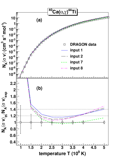
Figure 13: (Color online) (a) Data on the Maxwellian-averaged reaction rate for the ⁴⁰Ca($\alpha,\gamma$) reaction from Ref. vockenhuber07 are compared to calculations with inputs 1, 2, 7 and 8. (b) Ratio of the calculated reaction rates and experimental data. The upper dotted line indicates a 40% deviation from the experimental data, while the lower dotted line indicates a 20% deviation.

As seen here, all these four inputs give a reasonable reproduction of the measured rates, and they can hardly be distinguished from each other over the entire temperature range. We also note that the cross section range spans over ten orders of magnitude, and it is quite impressive how well the calculated rates follow the overall functional form of the data.

However, we observe that some models overestimate the rate somewhat, especially at higher temperatures. Now, the experimental rate could be too low for temperatures above $T_{9}\approx 4$ MeV because of missing resonances (only six resonances with measured resonance strengths are known for excitation energies at and above 9.3 MeV vockenhuber07 ). We note however that the rate at these high temperatures is not important for the final ⁴⁴Ti mass yield vockenhuber07 .

The combination of CT level density and standard GLO (input 7) gives a better reproduction of the DRAGON data at high temperatures than the others. However, this combination gave a too small average cross section as compared to the Nassar result. We therefore confirm the slight inconsistency between the two measurements, as discussed in Ref. vockenhuber07 . As already mentioned, we observed that the combination of the GHK level density and the averaged, standard GLO model (input 4) was not able to give a reasonable description of our primary $\gamma$ spectra for initial excitation energies above $\approx 7$ MeV. Therefore, input 8 cannot be recommended on the basis of the present data.

In order to get a clearer picture of the deviation of the calculated rates vs. the DRAGON data, the ratio of the calculated and experimental rate is shown in the lower panel of Fig. 13. Here, it is seen that input 7 gives the best fit to the DRAGON data for all temperatures above $T_{9}\approx 1.7$ ($T_{9}=10^{9}$ K). The large overestimate of the rate for $T_{9}<1.5$ is common for all model predictions and is due to problems with the $\alpha$ OMP at very low energies.

It is seen from the lower panel in Fig. 13 that all the calculated rates lie within 40% of the DRAGON data for $1.8\leq T_{9}\leq 4.5$, and for the 20% upper limit in the range $2.2\leq T_{9}\leq 3.7$. However, only input 7 (CT level density and standard GLO) is within the experimental error bars for $1.8\leq T_{9}\leq 4.5$.

It should be noted that by using the lower normalization limit for the RSF (blue, dashed-dotted line in Fig. 8), an excellent agreement with the DRAGON data is obtained. However, as stated previously, a good reproduction of the DRAGON data implies a too low integral cross section (in this case $\sigma_{\mathrm{ave}}=5.0$ $\mu$b) as compared to the Nassar data. On the other hand, using the upper normalization limit for the RSF (dashed line in Fig. 8), it is necessary to use the larger value of $f_{\mathrm{iso}}=8$ to obtain a reasonable agreement with the data (see Tab. 2).

To summarize, we have found that the model combinations input 1, input 2, and input 8 are in excellent agreement with the Nassar cross-section measurement. However, input 8 (GHK level density and standard GLO) is not in accordance with our primary $\gamma$ spectra for the relevant excitation-energy region ($E=7.2-9.3$ MeV) and should therefore not be used. The DRAGON data are best described with input 7 (CT level density and standard GLO) and the lower normalization limit of our RSF data (input 10). We also see that the small enhancement in the RSF at low $E_{\gamma}$ is not very important for the integrated cross section or the rate, as it gives a contribution of maximum 0.5 $\mu$b.

VI Summary

Particle-$\gamma$ coincidence data of the ⁴⁶Ti($p,t\gamma$)⁴⁴Ti reaction have been measured at OCL. By use of the Oslo method, primary $\gamma$-ray spectra have been extracted for initial excitation energies in the range $E=4.5-9.9$ MeV. From these spectra, the functional form of the level density and the RSF have been determined.

We have shown that a consistent normalization of the NLD and RSF is necessary in order to obtain a reasonable reproduction of the primary spectra. Also, the RSF seems to be independent of excitation energy and thus of the temperature, in accordance with the Brink hypothesis. However, the GLO model with a variable temperature, and averaged over the excitation-energy region, gives a rather good description of the overall shape of our RSF data when normalized to the CT level density.

Using input models consistent with our data give an excellent reproduction of the Nassar integral measurement of the ⁴⁰Ca($\alpha,\gamma$) reaction cross section. Also the DRAGON data of the reaction rate are rather well reproduced. However, we note that there is a discrepancy between the two datasets, so that it is not possible to use one model combination to obtain optimal agreement for both measurements simultaneously. Nevertheless, on the basis of our present data, it is clear that certain model combinations are not acceptable, although they might give reasonable results compared to the cross-section data.

- (1) C. Vockenhuber, C. O. Ouellet, L.-S. The, L. Buchmann, J. Caggiano, A. A. Chen, H. Crawford, J. M. D’Auria, B. Davids, L. Fogarty, D. Frekers, A. Hussein, D. A. Hutcheon, W. Kutschera, A. M. Laird, R. Lewis, E. O’Connor, D. Ottewell, M. Paul, M. M. Pavan, J. Pearson, C. Ruiz, G. Ruprecht, M. Trinczek, B. Wales, and A. Wallner, Phys. Rev. C 76, 035801 (2007).
- (2) M. Renaud, J. Vink, A. Decourchelle, F. Lebrun, P. R. den Hartog, R. Terrier, C. Couvreur, J. Knödlseder, P. Martin, N. Prantzos, A. M. Bykov, and H. Bloemen, Astrophys. Journal 647, L41L44 (2006).
- (3) A. F. Iyudin, R. Diehl, H. Bloemen, W. Hermsen, G. G. Lichti, D. Morris, J. Ryan, V. Schönfelder, H. Steinle, M. Varendorff, C. de Vries, and C. Winkler, Astron. Astrophysics 284, L1 (1994).
- (4) S. E. Woosley and T. A. Weaver, Astrophys. J. Suppl. Ser. 101, 181 (1995).
- (5) F.-K. Thielemann, K. Nomoto, and M. Hashimoto, Astrophys. J. 460, 408 (1996).
- (6) H. Nassar, M. Paul, I. Ahmad, Y. Ben-Dov, J. Caggiano, S. Ghelberg, S. Goriely, J. P. Greene, M. Hass, A. Heger, A. Heinz, D. J. Henderson, R. V. F. Janssens, C. L. Jiang, Y. Kashiv, B. S. Nara Singh, A. Ofan, R. C. Pardo, T. Pennington, K. E. Rehm, G. Savard, R. Scott, and R. Vondrasek, Phys. Rev. Lett. 96, 041102 (2006).
- (7) Data extracted from the -value calculator at the National Nuclear Data Center database, http://www.nndc.bnl.gov/qcalc/.
- (8) M. Guttormsen, A. Ataç, G. Løvhøiden, S. Messelt, T. Ramsøy, J. Rekstad, T.F. Thorsteinsen, T.S. Tveter, and Z. Zelazny, Phys. Scr. T 32, 54 (1990).
- (9) N. U. H. Syed, A. C. Larsen, A. Bürger, M. Guttormsen, S. Harissopulos, M. Kmiecik, T. Konstantinopoulos, M. Krtic̆ka, A. Lagoyannis, T. Lönnroth, K. Mazurek, M. Norrby, H. T. Nyhus, G. Perdikakis, S. Siem, and A. Spyrou, Phys. Rev. C 80, 044309 (2009).
- (10) J. Rapaport, J. B. Ball, R. L. Auble, T. A. Belote, and W. E. Dorenbusch, Phys. Rev. C 5, 453 (1972).
- (11) M. Guttormsen, T. S. Tveter, L. Bergholt, F. Ingebretsen, and J. Rekstad, Nucl. Instrum. Methods Phys. Res. A 374, 371 (1996).
- (12) M. Guttormsen, T. Ramsøy, and J. Rekstad, Nucl. Instrum. Methods Phys. Res. A 255, 518 (1987).
- (13) A. Schiller, L. Bergholt, M. Guttormsen, E. Melby, J. Rekstad, S. Siem, Nucl. Instrum. Methods Phys. Res. A 447 498 (2000).
- (14) A. C. Larsen, M. Guttormsen, M. Krtic̆ka, E. Běták, A. Bürger, A. Görgen, H. T. Nyhus, J. Rekstad, A. Schiller, S. Siem, H. K. Toft, G. M. Tveten, A. V. Voinov, and K. Wikan, Phys. Rev. C 83, 034315 (2011).
- (15) A. Bohr and B. Mottelson, Nuclear Structure, Benjamin, New York, 1969, Vol. I.
- (16) R. Chankova A. Schiller, U. Agvaanluvsan, E. Algin, L. A. Bernstein, M. Guttormsen, F. Ingebretsen, T. Lönnroth, S. Messelt, G. E. Mitchell, J. Rekstad, S. Siem, A. C. Larsen, A. Voinov, and S. Ødegård, Phys. Rev. C 73, 034311 (2006).
- (17) D. M. Brink, Ph.D. thesis, Oxford University, 1955.
- (18) A. Schiller and M. Thoennessen, At. Data Nucl. Data Tables 93, 549 (2007).
- (19) C. E. Porter and R. G. Thomas, Phys. Rev. 104, 483 (1956).
- (20) N. U. H. Syed, M. Guttormsen, F. Ingebretsen, A. C. Larsen, T. Lönnroth, J. Rekstad, A. Schiller, S. Siem, and A. Voinov, Phys. Rev. C 79, 024316 (2009).
- (21) S. Goriely, S. Hilaire, and A.J. Koning, Phys. Rev. C 78, 064307 (2008).
- (22) A. Gilbert and A. G. W. Cameron, Can. J. Phys. 43, 1446 (1965).
- (23) A.J. Koning, S. Hilaire, S. Goriely, Nucl. Phys. A810, 13 (2008).
- (24) A. J. Koning, S. Hilaire, and M. C. Duijvestijn, ”TALYS-1.2”, in Proceedings of the International Conference on Nuclear Data for Science and Technology, April 22-27, 2007, Nice, France. Editors: O. Bersillon, F. Gunsing, E. Bauge, R. Jacqmin, and S. Leray, EDP Sciences, 211 (2008). URL: http://www.talys.eu/
- (25) Data extracted using the NNDC On-Line Data Service from the ENSDF database, http://www.nndc.bnl.gov/ensdf/.
- (26) T. Belgya, O. Bersillon, R. Capote, T. Fukahori, G. Zhigang, S. Goriely, M. Herman, A. V. Ignatyuk, S. Kailas, A. Koning, P. Oblozinsky, V. Plujko and P. Young, Handbook for calculations of nuclear reaction data, RIPL-2. IAEA-TECDOC-1506 (IAEA, Vienna, 2006); also available online at http://www-nds.iaea.org/RIPL-2/
- (27) A. Voinov, E. Algin, U. Agvaanluvsan, T. Belgya, R. Chankova, M. Guttormsen, G.E. Mitchell, J. Rekstad, A. Schiller and S. Siem, Phys. Rev. Lett 93, 142504 (2004).
- (28) E. Algin, U. Agvaanluvsan, M. Guttormsen, A. C. Larsen, G. E. Mitchell, J. Rekstad, A. Schiller, S. Siem, and A. Voinov, Phys. Rev. C 78, 054321 (2008).
- (29) M. Guttormsen, R. Chankova, U. Agvaanluvsan, E. Algin, L.A. Bernstein, F. Ingebretsen, T. Lönnroth, S. Messelt, G.E. Mitchell, J. Rekstad, A. Schiller, S. Siem, A.C. Sunde, A. Voinov and S. Ødegård, Phys. Rev. C 71, 044307 (2005).
- (30) A. C. Larsen, R. Chankova, M. Guttormsen, F. Ingebretsen, T. Lönnroth, S. Messelt, J. Rekstad, A. Schiller, S. Siem, N. U. H. Syed, A. Voinov, and S. W. Ødegård, Phys. Rev. C 73, 064301 (2006).
- (31) A. C. Larsen, M. Guttormsen, R. Chankova, F. Ingebretsen, T. Lönnroth, S. Messelt, J. Rekstad, A. Schiller, S. Siem, N. U. H. Syed, and A. Voinov, Phys. Rev. C 76, 044303 (2007).
- (32) A. Voinov, S. M. Grimes, C. R. Brune, M. Guttormsen, A. C. Larsen, T. N. Massey, A. Schiller, and S. Siem, Phys. Rev. C 81, 024319 (2010).
- (33) F. Bec̆vár̆, Nucl. Instrum. Methods Phys. Res. A 417, 434 (1998).
- (34) C. Djalali et al., Nucl. Phys. A388, 1 (1982).
- (35) J. Kopecky and R. E. Chrien, Nucl. Phys. A468, 285 (1987).
- (36) J. Kopecky and M. Uhl, Phys. Rev. C 41 1941 (1990).
- (37) M. Krtic̆ka and F. Bec̆vár̆, J. Phys. G: Nuc. Part. Phys. 35, 014025 (2008).
- (38) S. A. Sheets, U. Agvaanluvsan, J. A. Becker, F. Bec̆vár̆, T. A. Bredeweg, R. C. Haight, M. Jandel, M. Krtic̆ka, G. E. Mitchell, J. M. O’Donnell, W. Parker, R. Reifarth, R. S. Rundberg, E. I. Sharapov, J. L. Ullmann, D. J. Vieira, J. B. Wilhelmy, J. M. Wouters, and C. Y. Wu, Phys. Rev. C 79, 024301 (2009).
- (39) A. C. Larsen and S. Goriely, Phys. Rev. C 82, 014318 (2010).
- (40) L. McFadden and G. R. Satchler, Nucl. Phys. 84, 177 (1966).
- (41) P. Demetriou, C. Grama, and S. Goriely, Nucl. Phys. A718, 510 (2003).
- (42) J. A. Holmes, S. E. Woosley, W. A. Fowler, and B. A. Zimmerman, At. Data Nucl. Data Tab. 18, 306 (1976).