The Equivalence of the Lagrangian-Averaged Navier-Stokes-$\alpha$ Model and the Rational LES model in Two Dimensions

Abstract

In the Large Eddy Simulation (LES) framework for modeling a turbulent flow, when the large scale velocity field is defined by low-pass filtering the full velocity field, a Taylor series expansion of the full velocity field in terms of the large scale velocity field leads (at the leading order) to the nonlinear gradient model for the subfilter stresses. Motivated by the fact that while the nonlinear gradient model shows excellent a priori agreement in resolved simulations, the use of this model by itself is problematic, we consider two models that are related, but better behaved: The Rational LES model that uses a sub-diagonal Pade approximation instead of a Taylor series expansion and the Lagrangian Averaged Navier-Stokes-$\alpha$ model that uses a regularization approach to modeling turbulence. In this article, we show that these two latter models are identical in two dimensions.

I Introduction

In a turbulent flow, it is usually the case that energy is predominantly contained at large scales where as a disproportionately large fraction of the computational effort is expended on representing the small scales in fully-resolved simulations of such flows (e.g., see Pope, 2000 Pope [2000]). Large eddy simulation (LES) is a technique that aims to explicitly capture the large, energy-containing scales while modeling the effects of the small scales that are more likely to be universal. This technique is both popular and is by far the most successful approach to modeling turbulent flows. We note, however, that in complex, wall-bounded and realistic configurations (such as, e.g., encountered in industrial situations), computational requirements for LES is still prohibitive that a hybrid (Reynolds Averaged Navier Stokes) RANS-LES approach is favored.Rajamani and Kim [2010]

The nature of the dynamics of large scale circulation in the world oceans and planetary atmospheres is quasi two dimensional due to constraints of geometry (small vertical to horizontal aspect ratio), rotation and stable stratification. For example, consider the (inviscid and unforced) quasi-geostrophic equations that describe the dynamics of the large, geostrophically and hydrostatically balanced, scales:

$${Dq\over Dt}={\partial q\over\partial t}+{\mathbf{u}}\cdot\nabla q=0$$ (1)

where $q$ is potential vorticity approximated in the quasi-geostrophic limit by

$$q=\nabla^{2}\psi+{\partial\over\partial z}\left({f_{0}^{2}\over N^{2}}{\partial\psi\over\partial z}\right)+\beta y,$$ (2)

and ${\mathbf{u}}$ is the advection velocity approximated in the quasi-geostrophic limit by the geostrophic velocity given in terms of streamfunction $\psi$ by ${\mathbf{u}}\approx{\mathbf{u}}_{g}={\mathbf{k}}\times\nabla\psi$. In other notation, $\nabla$ is the horizontal gradient operator, $f$ is the Coriolis parameter given by $f=f_{0}+\beta y$ in the $\beta$-plane approximation, $y$ is the meridional coordinate, $N^{2}$ is the Brunt-Vaisala frequency given in terms of the specified density gradient by $N^{2}={g\over\rho_{0}}{d\rho\over dz}.$ On the one hand, the particle-wise advection of potential-vorticity, and the dual conservation of (quadratic quantities) energy and potential-enstrophy are properties shared by quasi-geostrophic dynamics in common with two-dimensional flows. On the other hand, quasi-geostrophic dynamics shares in common with three-dimensional flow, the property of vortex stretching (in this limit, it is only the planetary vorticity $f_{0}$ that is stretched and is represented by the $\partial/\partial z$ term in (2).

It is the qualitative similarity of turbulence in these systems with two-dimensional turbulence, as elucidated by Charney, 1971, Charney [1971] that is the primary reason for interest in two-dimensional turbulence. The dual conservation of (potential) enstrophy and energy in (quasi) two-dimensional turbulence leads to profound differences as compared to fully three-dimensional turbulence: there exist two inertial regimes—a forward-cascade of (potential) enstrophy regime and an inverse-cascade of energy regime—in (quasi) two-dimensional turbulence in contrast to the single forward-cascade of energy regime in fully three-dimensional turbulence.

In the context of LES, which aims to model the effects of small-scales, it is clearly the forward-cascade inertial regimes that are of direct relevance. One of the most popular LES model is the Smagorinsky model,Smagorinsky [1963] and this class of eddy-viscosity models assume that the main effect of the unresolved scales is to remove, from the resolved scales, either energy for 3D flows or (potential) enstrophy for (quasi-geostrophic) 2D flows—the appropriate quantity that is cascading forward. However, an examination of the statistical distribution of the transfer of either energy in 3D turbulence or (potential) enstrophy in (quasi-geostrophic) 2D turbulence in the forward cascade regime[see Chen et al., 2003, Nadiga, 2008, 2009] demonstrates that the net forward cascade results from the forward-scatter being only slightly greater than the backscatter. Clearly, models such as the Smagorinsky model, or more generally scalar eddy-viscosity, by modeling only the net forward cascade, fail to represent possible important dynamical consequences of backscatter.

The recent reinterpretation of the classic work of Leray—which considered a mathematical regularization of the advective nonlinearity—in terms of the LES formalism, has given rise to the so-called regularization approach to modeling turbulence.${}^{\hbox{e.g., }}$ Geurts and Holm [2006] An important model in this approach is the Lagrangian-Averaged Navier-Stokes-$\alpha$ (LANS-$\alpha$) model introduced by Holm and co-workers.Holm et al. [1998]

The origins of the LANS-$\alpha$ turbulence model lie in 1) the notion of averaging over a fast turbulent spatial scale $\alpha$, the reduced-Lagrangian that occurs in the Euler-Poincare formalism of ideal fluid dynamics Holm et al. [1998], and in 2) three-dimensional generalizations Holm et al. [1998] of a nonhydrostatic shallow water equation system, known in literature as the Camassa-Holm equations. Chen et al. [1998] However, viewed from the point of view of the regularization approach, this model can be thought of as a particular frame-indifferent (coordinate invariant) regularization of the Leray type that preserves other important properties of the Navier-Stokes equations such as having a Kelvin theorem. To add to the richness of this model, almost exactly the same equations arise in the description of second-grade fluids Noll and Truesdell [1965], Graham et al. [2008] and vortex-blob methods.${}^{\hbox{e.g., }}$ Nadiga and Shkoller [2001]

There is now an extensive body of literature covering various aspects of the LANS-$\alpha$ model. In particular with respect to its turbulence modeling characteristics, analytical computation of the model shear stress profiles has shown favorable comparisons against laboratory data of turbulent pipe and channel flows Chen et al. [1998] and a posteriori comparisons of mixing in three-dimensional temporal mixing layer settings, Geurts and Holm [2006] in isotropic homogeneous turbulence settings, Chen et al. [1999], Mohseni et al. [2003] and in anisotropic settings Zhao and Mohseni [2005], Scott and Lien [2010] compare well against Direct Numerical Simulations (DNS). In three dimensions, it has, however, recently been noted Graham et al. [2008] that the use of LANS-$\alpha$ model as a subgrid model can be deficient in certain respects. In the two dimensional and quasi-two dimensional contexts, a posteriori comparisons of LANS-$\alpha$ based computations have shown favorable comparisons against eddy-resolving computations. Nadiga and Margolin [2001], Holm and Nadiga [2003], Hecht et al. [2008] Nevertheless, this model has mostly been viewed as a complementary approach to modeling turbulence.

The nonlinear gradient model Leonard [1974], Clark et al. [1979], Meneveau and Katz [2000] and the Rational LES model Galdi and Layton [2000], Iliescu et al. [2003], Berselli et al. [2006] are part of another class of LES models, built on a direct dynamical analysis of what should be a good approximation of the effect of the subgrid scales on the largest scales, through turbulent stresses. When the large scale velocity field is defined by low-pass filtering the velocity field, a natural asymptotic expansion leads to approximated turbulent stresses. This defines the nonlinear gradient model. An essential point is that the actual turbulent stresses of 2D and quasi-geostrophic turbulent flows, computed from direct numerical simulation, have been shown to be well approximated by the one defining the nonlinear gradient model. Bouchet [2001], Chen et al. [2003], Nadiga [2008, 2009]

The nonlinear gradient model (11) uses a natural approximation of the turbulent stresses. However this model has several drawbacks. Indeed, whereas it has been proven that the nonlinear gradient model turbulent stress (11) preserves energy for two dimensional flows, Bouchet [2001] this is generally not the case in three dimensional flows, and instabilities or finite time energy blow up can occur. The situation is not much better in 2D and quasi-geostrophic flows in that the incompressiblity constraint implies that the divergence of the deformation tensor ($\sigma$ in equation (11)) generally has a positive definite direction and a negative definite direction. Physically, this amount to an anistropic viscosity with positive value in some directions and negative values in other directions. Bouchet [2001], Chen et al. [2003], Nadiga [2008, 2009] These drawbacks mean that the nonlinear model is not a good physical model and will lead to instabilities, for two dimensional, quasi-geostrophic and three dimensional flows. An alternative model based on entropic closures, keeping the main properties of the nonlinear model (good approximation of the turbulent stresses, conservation of energy), has been proposed and proven to give very good results for two-dimensional flows. Bouchet [2001] In three dimensions, Domaradzki and Holm, 2001, Domaradzki and Holm [2001] note that one component of the LANS-$\alpha$ (subfilter stress) model corresponds to the subfilter stress that would be obtained upon using an approximate deconvolution procedure on the nonlinear gradient model.

Analysis of the drawbacks of the nonlinear gradient model led Galdi and Layton to propose the Rational LES model. Galdi and Layton [2000] The Rational LES model coincides with the nonlinear model at leading order, but provides a stronger attenuation of the smallest scale. As confirmed by recent mathematical results, Berselli et al. [2006] the Rational LES model is well posed and should lead to stable numerical algorithms. It is thus a good candidate for LES.

The Nonlinear-Gradient model has been well studied over more than three decades. These studies started with Leonard, 1974 Leonard [1974] and Clark, Ferziger and Reynolds, 1979. Clark et al. [1979] Rather than attempt an incomplete survey of the literature relevant to the a priori and a posteriori testing of this model here, we note that a fairly modern account of this can be found in Meneveau and Katz, 2000.Meneveau and Katz [2000] The more recent aspect of the Rational LES model is in making the highly favorable a priori comparisons of the Nonlinear-Gradient model more amenable to a posteriori simulations. For example, Iliescu et al., 2003Iliescu et al. [2003] compare the behavior of the Rational LES model to the Nonlinear Gradient model (and the Smagorinski model) in the 2D and 3D cavity flow settings, both at low and high Reynolds numbers. They find a) that laminar flows are correctly simulated by both models, and b) that at high Reynolds numbers, the Nonlinear Gradient model simulations, either with or without the Smagorinski model, lead to a finite time blow-up while the Rational LES model simulation displayed no such problem and succeeded in its LES role, i.e., compared to a fine-scale resolved simulation, the Rational LES model was able to capture and model the large-eddies well on a coarse mesh. Furthermore, they find that the Rational LES model performed better than the Smagorinski model alone in capturing the behavior of the large-eddies. Finally, we note that with both the Rational LES model and the LANS-$\alpha$ models, the burden of modeling borne by the additional dissipative term is smaller than in other approaches.

Following the development of these models, we note that the LANS-$\alpha$ and the rational LES model have interesting complementary properties: While the LANS-$\alpha$ preserves the Euler equation structure through the Kelvin theorem, the Rational LES model develops a good approximation of the turbulent stresses while ameliorating problems associated with the nonlinear gradient model. It would thus be useful to examine the relation between these two models. In this article, we demonstrate the equivalence of the LANS-$\alpha$ to the Rational LES model in two-dimensions. By equivalence, we mean here that, the evolution equations for one of the models can be exactly transformed into the other. As will be evident, given the very different approaches taken in arriving at these models, it’ll involve more than a simple transformation; it will also involve disentangling the turbulence term implied by the particular regularization of the nonlinear term. The importance of this result lies in the fact that mathematical results obtained for one of these models become also true for the other. We also demonstrate that these two models are different in three dimensions.

In sections 1 and 2, after recalling the framework of turbulent stresses and LES, we briefly describe the nonlinear gradient, the Rational LES, and the LANS-$\alpha$ models. In section 3, we prove the equivalence of the Rational LES and of the LANS-$\alpha$ models in two dimensions. In section 4, we prove that they are not equivalent in three dimensions. After a brief numerical example, implications of the above results are discussed in the final section.

II LES of Two-Dimensional Turbulence and the nonlinear-gradient model

In LES, the resolution of energy containing eddies that dominate flow dynamics is made computationally feasible by introducing a formal scale separation. Pope [2000] The scale separation is achieved by applying a low-pass filter $G$ with a characteristic scale $\alpha$ ($2\alpha^{2}$ is the second moment of $G$) to the original equations. To this end, let the fields ${\mathbf{u}}$, $q$, etc… be split into large-scale (subscript $l$)and small-scale (subscript $s$) components as

$${\mathbf{u}}={\mathbf{u}}_{l}+{\mathbf{u}}_{s},$$

where

$${\mathbf{u}}_{l}({\mathbf{x}})=\int_{D}G({\mathbf{x}}-{\mathbf{x}}^{\prime}){\mathbf{u}}({\mathbf{x}}^{\prime})d{\mathbf{x}}^{\prime},$$

$${\mathbf{u}}_{s}({\mathbf{x}})={\mathbf{u}}-{\mathbf{u}}_{l},$$

the filter function $G$ is normalized so that

$$\int_{D}G({\mathbf{x}}^{\prime})d{\mathbf{x}}^{\prime}=1,$$

and where the integrations are over the full domain $D$. In contrast to Reynolds decomposition, however, generally, ${\mathbf{u}}_{ll}\neq{\mathbf{u}}_{l}$ and ${\mathbf{u}}_{sl}\neq 0$.

For convenience, we write the two-dimensional vorticity equation as

$${D\omega\over Dt}={\partial\omega\over\partial t}+{\mathbf{u}}\cdot\nabla\omega=\nabla\times F_{2d}+\nabla\times D_{2d}=F+D,$$ (3)

where $F_{2d}$ is the two-dimensional momentum forcing, $D_{2d}$ is dissipation, and where, for brevity, we denote $\nabla\times F_{2d}$ by $F$, and $\nabla\times D_{2d}$ by $D$. Applying the filter to (3) leads to an equation for the evolution of the large-scale component of vorticity which is the primary object of interest in LES:

$${\partial\omega_{l}\over\partial t}+\nabla\cdot\left({\mathbf{u}}_{l}\omega_{l}\right)=F_{l}+D_{l}-\nabla\cdot\mathbf{\sigma}$$ (4)

where

$$\mathbf{\sigma}=\left({\mathbf{u}}\omega\right)_{l}-{\mathbf{u}}_{l}\omega_{l}$$ (5)

is the turbulent sub-filter vorticity-flux, and as in (3), we denote $\left(\nabla\times F_{2d}\right)_{l}$ by $F_{l}$, and so also for dissipation. This turbulent subgrid vorticity-flux may in turn be written in terms of the Leonard stress, cross-stress, and Reynolds stress Pope [2000] as

$$\sigma=\underbrace{({\mathbf{u}}_{l}\omega_{l})_{l}-{\mathbf{u}}_{l}\omega_{l}}_{\hbox{Leonard stress}}+\underbrace{({\mathbf{u}}_{l}\omega_{s})_{l}+({\mathbf{u}}_{s}\omega_{l})_{l}}_{\hbox{Cross-stress}}\quad\quad+\underbrace{({\mathbf{u}}_{s}\omega_{s})_{l}}_{\hbox{Reynolds stress}}.$$ (6)

However, while $\sigma$ itself is Galilean-invariant, the above Leonard- and Cross-stresses are not Galilean-invariant. Thus when these component stresses are considered individually, the following decomposition, originally due to Germano, 1986Germano [1986] is preferable

$$\sigma=\underbrace{({\mathbf{u}}_{l}\omega_{l})_{l}-{\mathbf{u}}_{ll}\omega_{ll}}_{\hbox{Leonard Stress}}+\underbrace{({\mathbf{u}}_{l}\omega_{s})_{l}+({\mathbf{u}}_{s}\omega_{l})_{l}-{\mathbf{u}}_{ll}\omega_{sl}-{\mathbf{u}}_{sl}\omega_{ll}}_{\hbox{Cross-stress}}+\underbrace{({\mathbf{u}}_{s}\omega_{s})_{l}-{\mathbf{u}}_{sl}\omega_{sl}}_{\hbox{Reynolds stress}}.$$ (7)

The filtered equations, which are the object of simulation on a grid with a resolution commensurate with the filter scale in LES, are then closed by modeling subgrid-scale (SGS) stresses to account for the effect of the unresolved small-scale eddies. In this case (4) will be closed on modeling the turbulent subgrid vorticity-flux $\mathbf{\sigma}$.

As is tradition, a Gaussian filter is chosen. In eddy-permitting simulations, some of the range of scales of turbulence are explicitly resolved. Therefore, information about the structure of turbulence at these scales is readily available. In LES formalism, there is a class of models that attempt to model the smaller unresolved scales of turbulence based on the assumption that the structure of the turbulent velocity field at scales below the filter scale is the same as the structure of the turbulent velocity field at scales just above the filter scale. Meneveau and Katz [2000]

Further expansion of the velocity field in a Taylor series and performing filtering analytically results in

$$(u_{i}u_{j})_{l}\propto{\partial u_{li}\over\partial x_{k}}{\partial u_{lj}\over\partial x_{k}},$$ (8)

a quadratic nonlinear combination of resolved gradients for the subgrid model. Leonard [1974], Clark et al. [1979] The interested reader is referred to Meneveau and Katz, 2000Meneveau and Katz [2000] for a comprehensive review of the nonlinear-gradient model.

Equivalently, expansion of ${\mathbf{u}}_{l}$ and $\omega_{l}$ in the Galilean-invariant form of the Leonard-stress component of the sub-filter eddy-flux of vorticity (7) in a Taylor series:

$$({\mathbf{u}}_{l}\omega_{l})_{l}-{\mathbf{u}}_{ll}\omega_{ll}=$$

$$=\int d{\mathbf{x}}^{\prime}\;G({\mathbf{x}}-{\mathbf{x}}^{\prime})\left({\mathbf{u}}_{l}({\mathbf{x}})+(x^{\prime}-x)_{j}{\partial u_{li}\over\partial x_{j}}({\mathbf{x}})\right)\left(\omega_{l}({\mathbf{x}})+(x^{\prime}-x)_{j}{\partial\omega_{l}\over\partial x_{j}}({\mathbf{x}})\right)-$$

$$\int d{\mathbf{x}}^{\prime}\;G({\mathbf{x}}-{\mathbf{x}}^{\prime})\left({\mathbf{u}}_{l}({\mathbf{x}})+(x^{\prime}-x)_{j}{\partial u_{li}\over\partial x_{j}}({\mathbf{x}})\right)*\int d{\mathbf{x}}^{\prime}\;G({\mathbf{x}}-{\mathbf{x}}^{\prime})\left(\omega_{l}({\mathbf{x}})+(x^{\prime}-x)_{j}{\partial\omega_{l}\over\partial x_{j}}({\mathbf{x}})\right)$$

produces at the first order

$$\sigma=2\alpha^{2}{\partial u_{li}\over\partial x_{j}}\;{\partial\omega_{l}\over\partial x_{i}}+\mathcal{O}(\alpha^{4})=2\alpha^{2}\nabla{\mathbf{u}}_{l}\cdot\nabla\omega_{l}+\mathcal{O}(\alpha^{4}),$$ (9)

where $2\alpha^{2}$ is the second moment of the filter used. The leading order is again a quadratic nonlinear combination of resolved gradients. The approximate model that retains only the second order term is called the nonlinear gradient model. In this two-dimensional setup, it reads

$$\frac{\partial\omega_{l}}{\partial t}+\mathbf{u}_{l}\bm{\cdot\nabla}\omega_{l}=-2\alpha^{2}\left[\nabla\mathbf{u}_{l}^{T}.\nabla(\nabla\omega_{l})\right]+F_{l}+D_{l}$$ (10)

(please see the appendix for the definition of operator $\nabla\mathbf{u}_{l}^{T}.\nabla$).

For simplicity, we have presented the two-dimensional derivation of the nonlinear gradient model, however similar considerations lead to the three dimensional nonlinear gradient model:

$$\frac{\partial{\mathbf{u}}_{l}}{\partial t}+{\mathbf{u}}_{l}\bm{\cdot\nabla}{\mathbf{u}}_{l}=-2\alpha^{2}\bm{\nabla\cdot}\left[\nabla{\mathbf{u}}_{l}\nabla{\mathbf{u}}_{l}\right]-\bm{\nabla}P+\left(F_{3d}\right)_{l}+\left(D_{3d}\right)_{l}.$$ (11)

In the two dimensional context, this model has been derived by Eyink, 2001 Eyink [2001] without the self-similarity assumption, but rather by assuming scale-locality of contributions to $\mathbf{\sigma}$ at scales smaller than the filter scale, and its use has been investigated by various authors. Bouchet [2001], Chen et al. [2003] Nadiga, 2008 and 2009Nadiga [2008, 2009] have demonstrated excellent a priori testing of the nonlinear gradient model in quasi-geostrophic turbulence, the same also holds in the three-dimensional turbulence context.${}^{\hbox{e.g., }}$ Meneveau and Katz [2000] The nonlinear gradient model, however, holds much better in two-dimensional and quasi two-dimensional settings than in fully three-dimensional settings.

III Rational LES model and the LANS-$\alpha$ model

III.1 Rational LES model

By analyzing the nonlinear-gradient model in terms of Fourier components, Galdi and Layton, noted that the nonlinear-gradient model increases the high wavenumber components (scales smaller than the filter scale) and therefore does not ensure that $\omega_{l}$ is smoother than $\omega$. Consequently, to remedy this problem, they proposed an approximation which attenuates the small scale eddies, but is of the same order accuracy for large eddies (the two approximations coincide at order $\alpha^{2}$, see (11)).

To this end, rather than using a Taylor expansion of the filter ($e^{-bx^{2}}\approx 1-bx^{2}$), they considered the rational approximation

$$e^{-bx^{2}}\approx{1\over 1+bx^{2}}$$ (12)

Using the above sub-diagonal Pade approximation, the modified nonlinear-gradient model leads to the ’Rational LES’ model. We refer to Galdi and Layton, 2000Galdi and Layton [2000] for the derivation of the evolution equation for ${\mathbf{u}}_{l}$ (which is an approximation of the large scale component of the full velocity field ${\mathbf{u}}$.) It is

$$\frac{\partial{\mathbf{u}}_{l}}{\partial t}+{\mathbf{u}}_{l}\bm{\cdot\nabla}{\mathbf{u}}_{l}=-2\alpha^{2}\left(I-\alpha^{2}\Delta\right)^{-1}\bm{\nabla\cdot}\left[\nabla{\mathbf{u}}_{l}\nabla{\mathbf{u}}_{l}\right]-\bm{\nabla}P+\left(F_{3d}\right)_{l}+\left(D_{3d}\right)_{l},$$ (13)

with $\bm{\nabla\cdot}{\mathbf{u}}_{l}=0$, and where $\left(I-\alpha^{2}\Delta\right)^{-1}$ is the inverse of the operator $\left(I-\alpha^{2}\Delta\right)$ (easily expressed in a Fourier basis).

III.2 The LANS-$\alpha$ model

In the context of the three-dimensional incompressible Navier-Stokes equations

$${\partial{\mathbf{u}}\over\partial t}+{{\mathbf{u}}}\cdot\nabla{\mathbf{u}}=-\nabla\phi+F_{3d}+\nu\Delta{\mathbf{u}}~{}~{}~{};~{}~{}~{}\nabla\cdot{\mathbf{u}}=0,$$ (14)

on a suitable domain with appropriate boundary conditions, Leray regularization of (14) is expressed by ${}^{\hbox{e.g., }}$ Geurts and Holm [2006]

$${\partial{\mathbf{u}}\over\partial t}+{{\mathbf{u}}_{l}}\cdot\nabla{\mathbf{u}}=-\nabla\phi+F_{3d}+\nu\Delta u,$$ (15)

where ${{\mathbf{u}}_{l}}$ is the large scale component of velocity filtered at a characteristic length $\alpha$, $\phi=p/\rho_{0}$ is the normalized pressure, $F_{3d}$ is the external forcing and $\nu$ the kinematic viscosity. The filtered velocity ${{\mathbf{u}}_{l}}$ can be obtained by application of a convolution filter to ${\mathbf{u}}$. A particularly important example is the Helmholtz filter, to which we turn momentarily. The Leray approach is basic to many recent studies in regularized turbulence. This regularization model does not preserve some of the properties of the original equations (14), such as a Kelvin circulation theorem. This is where the LANS-$\alpha$ formulation provides an important extension.

A transparent way to present the LANS-$\alpha$ model is obtained when the incompressible Navier-Stokes (momentum) equations are written in the equivalent form

$${\partial{\mathbf{u}}\over\partial t}-{{\mathbf{u}}}\times\left(\nabla\times{\mathbf{u}}\right)=-\nabla\phi+F_{3d}+\nu\Delta{\mathbf{u}}.$$ (16)

The LANS-$\alpha$ model is then given by ${}^{\hbox{e.g., }}$ Holm et al. [1998], Geurts and Holm [2006]

$${\partial{\mathbf{u}}\over\partial t}-{{\mathbf{u}}_{l}}\times\left(\nabla\times{\mathbf{u}}\right)=-\nabla\phi+F_{3d}+\nu\Delta{\mathbf{u}}.$$ (17)

Thus, just as the Leray regularization corresponds to the filtering of the advecting velocity, the LANS-$\alpha$ regularization amounts to filtering the velocity in the nonlinear term when written as the direct product of a velocity and a vorticity ${\bm{\omega}=\nabla\times{\mathbf{u}}}$. The LANS-$\alpha$ model may be written in the more common advective nonlinearity form

$$\frac{\partial{\mathbf{u}}}{\partial t}+{\mathbf{u}_{l}}\cdot\nabla{\mathbf{u}}-\alpha^{2}\left(\nabla{{\mathbf{u}}_{l}}\right)^{T}\Delta{{\mathbf{u}}_{l}}=-\nabla p+F_{3d}+\nu\Delta{\mathbf{u}}.$$ (18)

The filtered velocity is obtained by an inversion of the Helmholtz operator: ${{\mathbf{u}}_{l}}{=(1-\alpha^{2}\Delta)^{-1}{\mathbf{u}}}$ with appropriate boundary conditions. (It has to be noted that in a non-periodic domain, the boundary conditions that are necessary to invert the Helmholtz operator are specific to this modeling procedure.) The third term on the left in (18) is introduced in the LANS-$\alpha$ modeling approach to restore a Kelvin theorem to the modeled equations.

It is also instructive to consider the evolution of vorticity. For the Navier-Stokes equation, vorticity evolution is

$$\frac{\partial\bm{\omega}}{\partial t}+{\mathbf{u}}\cdot\nabla\bm{\omega}=\bm{\omega}\cdot\nabla{\mathbf{u}}+\nabla\times F_{3d}+\nu\Delta\bm{\omega}.$$ (19)

The vorticity evolution corresponding to the LANS-$\alpha$ model is

$$\frac{\partial\bm{\omega}}{\partial t}+{\mathbf{u}_{l}}\cdot\nabla\bm{\omega}=\bm{\omega}\cdot\nabla{\mathbf{u}}_{l}+\nabla\times F_{3d}+\nu\Delta\bm{\omega},$$ (20)

where in addition to a filtered advecting velocity, a mollification of the vortex-stretching term is evident.

In two dimensions, (20) reduces to

$$\frac{\partial{\omega}}{\partial t}+{\mathbf{u}_{l}}\cdot\nabla{\omega}=\nabla\times F_{2d}+\nabla\times D_{2d}=F+D,$$ (21)

where forcing and dissipation have been written in correspondance with the notation used in the two dimensional vorticity equation (3) and its LES counterpart (4).

IV Identity of the Rational LES and LANS-$\alpha$ models in two dimensions

In this section, we consider the Rational LES model and the LANS-$\alpha$ models in two-dimensions. Taking the curl of the two-dimensional velocity equation for the Rational LES model (13), we obtain the vorticity equation

$$\frac{\partial\omega_{l}}{\partial t}+\mathbf{u}_{l}\bm{\cdot\nabla}\omega_{l}=-2\alpha^{2}\left(I-\alpha^{2}\Delta\right)^{-1}\left[\nabla\mathbf{u}_{l}^{T}.\nabla(\nabla\omega_{l})\right]+F_{l}+D_{l},$$ (22)

where $\omega_{l}$ is the vertical component of $\bm{\omega}_{l}$. In order to compare the Rational LES model (22) with the LANS-$\alpha$ model (21), we apply operator $\left(I-\alpha^{2}\Delta\right)$ to (22) and write the evolution equation for $\omega$ as

$$\frac{\partial\omega}{\partial t}+\mathbf{u}_{l}\bm{\cdot\nabla}\omega=\delta M+F+D.$$ (23)

Comparing (23) with (21), we note that $\delta M$ is the difference between the two models and is given by

$$\delta M=-2\alpha^{2}\left[\nabla\mathbf{u}_{l}^{T}.\nabla(\nabla\omega_{l})\right]+\mathbf{u}_{l}\bm{\cdot\nabla}\left[\left(I-\alpha^{2}\Delta\right)\omega_{l}\right]-\left(I-\alpha^{2}\Delta\right)\left[\mathbf{u}_{l}\bm{\cdot\nabla}\omega_{l}\right].$$

By direct computation this expression simplifies to

$$\delta M=\alpha^{2}\left\{-2\left[\nabla\mathbf{u}_{l}^{T}.\nabla(\nabla\omega_{l})\right]-\mathbf{u}\bm{\cdot\nabla}\left[\Delta\omega_{l}\right]+\Delta\left[\mathbf{u}_{l}\bm{\cdot\nabla}\omega_{l}\right]\right\}.$$

Then using the vector calculus identity (29) in the appendix, we conclude that $\delta M=0$. The dynamics of $\omega$ is thus the same as given by the $LANS-\alpha$ model

$$\frac{\partial\omega}{\partial t}+\mathbf{u}_{l}\bm{\cdot\nabla}\omega=F+D.$$

We thus conclude that the Rational LES model and the LANL-$\alpha$ models are equivalent in two dimensions.

V The Rational LES and LANS-$\alpha$ models are different in three dimensions

In three dimensions, the Rational LES model for an incompressible flow ($\nabla.\mathbf{u}=0$) is

$$\frac{\partial\mathbf{u}_{l}}{\partial t}-\mathbf{u}_{l}\bm{\times}\left(\nabla\bm{\times}\mathbf{u}_{l}\right)=-\frac{\mbox{$\nabla$}P_{1}}{\rho}-2\alpha^{2}\left(I-\alpha^{2}\Delta\right)^{-1}\left[\nabla\mathbf{u}_{l}^{T}.\nabla(\nabla\mathbf{u}_{l})\right]+\left(F_{3d}\right)_{l}+\nu\Delta{\mathbf{u}}_{l},$$ (24)

where $P_{1}$ is the sum of the physical and kinetic pressure. The LANS-$\alpha$ model is

$$\frac{\partial\mathbf{u}}{\partial t}-\mathbf{u}_{l}\bm{\times}\left(\nabla\bm{\times}\mathbf{u}\right)=-\frac{\mbox{$\nabla$}P_{2}}{\rho}+F_{3d}+\nu\Delta{\mathbf{u}},$$ (25)

where $\mathbf{u}=\left(I-\alpha^{2}\Delta\right)\mathbf{u}_{l}$.

Applying the operator $\left(I-\alpha^{2}\Delta\right)$ to (24), we obtain the equation verified by $\mathbf{u}=\left(I-\alpha^{2}\Delta\right)\mathbf{u}_{l}$ in the case of the Rational LES model:

$$\frac{\partial\mathbf{u}}{\partial t}-\mathbf{u}_{l}\bm{\times}\left(\nabla\bm{\times}\mathbf{u}\right)=-\frac{\mbox{$\nabla$}P_{3}}{\rho}+\mathbf{N}+F_{3d}+\nu\Delta{\mathbf{u}},$$ (26)

with $P_{3}=\left(I-\alpha^{2}\Delta\right)P_{2}$, and with

$$\mathbf{N}=\alpha^{2}\left\{-2\nabla\mathbf{u}_{l}^{T}.\nabla(\nabla\mathbf{u}_{l})+\mathbf{u}_{l}\times\bm{\nabla}\times\left[\Delta\mathbf{u}_{l}\right]+\Delta\left[\mathbf{u}_{l}\times\left(\bm{\nabla}\times\mathbf{u}_{l}\right)\right]\right\}.$$

The two equations (25) and (26) are equivalent if and only if $\mathbf{N}$ is a gradient, that is if and only if $\nabla\times\mathbf{N}=0$. For two-dimensional vector-fields, we have proven in the section above that $\delta M\mathbf{e}_{z}=\nabla\times\mathbf{N}=0$. In contrast this is wrong in general for three-dimensional vector fields, because of vortex-stretching type terms present for three dimensional vector fields and non-present for two dimensional vector fields. In order to prove this we give below an example of field $\mathbf{u}_{l}$ for which $\nabla\times\mathbf{N}\neq 0$.

Consider for example $\mathbf{u}_{l}=y^{2}\mathbf{e}_{x}-xz\mathbf{e}_{y}+xy\mathbf{e}_{z}$. Then $\mathbf{u}_{l}$ is actually non-divergent: $\nabla\cdot\mathbf{u}_{l}=0$. By direct computation, we have $\bm{\nabla}\times\left[\Delta\mathbf{u}_{l}\right]=0$, $\mathbf{u}_{l}\times\bm{\nabla}\times\left[\Delta\mathbf{u}_{l}\right]=0$, $\nabla\times\left[\nabla\mathbf{u}_{l}^{T}.\nabla(\nabla\mathbf{u}_{l})\right]=2\mathbf{e}_{x}$, $\nabla\times\left\{\Delta\left[\mathbf{u}_{l}\times\left(\bm{\nabla}\times\mathbf{u}_{l}\right)\right]\right\}=-8\mathbf{e}_{x}$ and then $\nabla\times\mathbf{N}=4\alpha^{2}\mathbf{e}_{x}\neq 0$.

We thus conclude that the Rational LES and the LANS-$\alpha$ models are not equivalent in three dimensions.

VI A numerical example

The primary emphasis of this article is the above analytical demonstration of the equivalence of the Rational LES model and the LANS-$\alpha$ model in two dimensions rather than an evaluation of the performance of the model(s) considered. Nevertheless, at the insistence of one of the referees, we briefly present an example computation in two dimensions in this section.

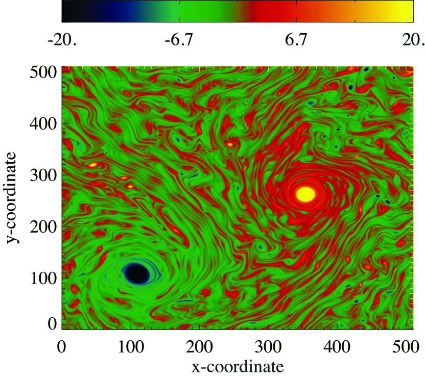
Figure 1: Snaphot of vorticity field of reference run at statistical stationarity. The stochastic forcing is confined to a band of wavenumbers between 15 and 16 (domain is $2\pi\times 2\pi$) and dissipation consists of a combination of Rayleigh friction and hyperviscosity.

We consider a (stochastically) forced-dissipative flow in a doubly period domain $2\pi$ on the side. As is conventional in numerous earlier investigations of two dimensional turbulence, dissipation $D$ consists of linear damping: $-r\omega$, where $r(=10^{-3})$ is a frictional constant, and an eigth order hyperviscous term that acts as a sink of the net-forward cascading enstrophy. Forcing $F$ is scaled as $F=\sqrt{2r}\tilde{F}$, where $\tilde{F}$ is an isotropic stochastic forcing in a small band of wavenumbers $15\leq k_{f}<16$ drawn from an independent unit variance Gaussian distribution and which is temporally uncorrelated: $\left<\tilde{F}_{\mathbf{k}}(t)\tilde{F}_{\mathbf{k}^{\prime}}(t^{\prime})\right>=\delta_{\mathbf{k}\mathbf{k}^{\prime}}(t-t^{\prime})$. A fully-dealiased pseudo spectral spatial discretization is used in conjunction with an adaptive fourth-fifth order Runge-Kutta Cash-Karp time stepping scheme. The time step used ensures that the relative error of the time increment is less that $10^{-6}$, and with the time step ending up being much smaller than that required by stability requirements.

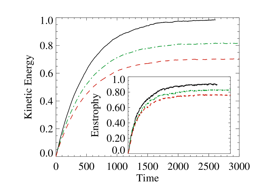
Figure 2: The evolution of kinetic energy and enstrophy (inset) in the reference run (solid line; black), bare truncation run (dashed line; red) and the LES run (dot-dashed line; green). The horizontal axis in the inset spans the same range of times as in the main plot. The former uses a 512x512 physical space grid where as the latter two runs use a 128x128 grid. The changes introduced by the subgrid model are so as to improve the bare truncation run in the direction of the reference run.

For the reference computation, a 512x512 physical grid is chosen giving a gridsize of $\pi/256$. Figure 1 shows the vorticity field after the flow has equilibrated (at $t$=2600 eddy turnover times.) Given the stochastic forcing and the turbulent nature of the flow, a statistical consideration of the flow is in order: The evolution of the domain integrated kinetic energy and enstrophy as a function of time is shown in Fig. 2. Figure 3 shows the one-dimensional spectral density of kinetic energy and the spectral flux of kinetic energy ($\int_{0}^{k}2\pi k\,dk\,\hbox{Re}({\widehat{{\mathbf{u}}}}^{*}{\mathbf{\cdot}}{\widehat{{\mathbf{u}}{\mathbf{\cdot}}{\mathbf{\nabla}}{\mathbf{u}}}})$ where $\hbox{Re}(.)$ denotes the real part, ${\widehat{.}}$ denotes the Fourier transform and superscript $*$ denotes complex conjugate.) For the spectral flux of kinetic energy diagnostic, we verify that the integral over all wavenumbers goes to zero to within roundoff. Note that the x-axis in Fig. 3 is truncated at wavenumber 60 to better focus on the range of scales of interest. In all these figures, the solid line represents the reference run.

Next, we choose a filter width of $\pi/32$, and following arguments similar to those in section 13.2 of Pope, 2000 Pope [2000], we choose an LES gridsize of $\pi/64$ (that corresponds to a 128x128 physical grid.) On the (coarser) LES grid, we perform two simulations: One that we call a bare truncation—(22), but without the first term on the right hand side–and a second one with the LES model discussed above—(22)—with the rest of the setup being identical. The evolution of domain-integrated kinetic energy and enstrophy and the spectral density and spectral flux density of kinetic energy for these two simulations are shown again in Figs. 2 and 3. The bare truncation run in these figures is shown by dashed (red) lines, whereas the Rational LES or LANS-$\alpha$ model runs are shown by dot-dashed (green) lines.

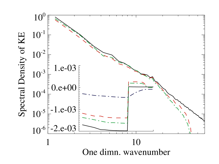
Figure 3: The one-dimensional power spectral density (logarithmic scale) and spectral flux density (inset; linear scale) plotted as a function of the one-dimensional wavenumber (logarithmic scale). The horizontal axis in the inset spans the same range of wavenumbers as in the main plot. Reference run: solid line, black; bare truncation run: dashed line, red; and the LES run: dot-dashed line, green. The thick dot-dashed line in blue in the inset corresponds to the spectral flux of energy due to the subgrid model. In the range of scales where there is an inverse cascade of energy, the LES run is more energetic than the bare truncation run, and the LES run closely follows the reference run. However at the small scales, the energy spectrum of the LES run falls off faster than the bare truncation run (at these range of scales, the reference run is still inertial.) The increased level of energy at the large scales in the LES run is seen as due to a secondary inverse cascade that is put in place by the subgrid model (backscatter). In effect, as compared to the bare truncation run, in the LES run, the forward cascade of energy is reduced and the inverse cascade of energy is augmented.

In each of these diagnostics, the tendency of the model to improve on the bare truncation is evident. In the spectral density plot, on comparing the bare truncation with the model simulation, the tendency of the model to deemphasize the small scales while increasing the energy in the large scales is seen. The dynamics of how this is achieved is seen to be that of an augmentation of the inverse cascade by the model term as indicated by the blue line in the spectral flux inset. The net result is that the full nonlinear flux of energy shows a smaller forward cascade and an increased inverse cascade, as compared to the bare truncation simulation. And these changes in the spectral flux of energy are in the direction of bridging the (coarser) bare truncation run to the reference simulation. We note that a) we did not tune any of the parameters to match the reference run; we anticipate that with tuning, the LES results could better match the reference run, and that b) the computations on the LES grid are about 60 to 100 times less computationally intensive as compared to the reference run, with the overhead for the model (over bare truncation) being negligible.

VII Conclusion

In its popular form, the LES approach to modeling turbulence comprises of applying a filter to the original set of equations; the nonlinear terms then give rise to unclosed residual terms that are then modeled. However, the regularization approach to modeling turbulence consists of, besides other possible considerations, a modification of the nonlinear term based on filtering of one of the fields. The latter approach, however, implies a model of the unclosed residual terms when viewed from the point of view of the former. We consider the Rational LES model Galdi and Layton [2000] that falls under the former approach, and the LANS-$\alpha$ model Holm et al. [1998] that falls under the latter approach. In this article, we demonstrate that the two models are equivalent in two dimensions, but not in three dimensions. Their equivalence in two dimensions allows arguments about the mathematical structure and physical phenomenology of either of the models to be equally valid for the other.

VIII Appendix

We derive in this appendix calculus identities for two-dimensional or three-dimensional vector fields. We define for any vector fields $\mathbf{A}$ and scalar $B$: $\nabla\mathbf{A}^{T}.\nabla(\nabla B)\equiv\partial_{i}A_{j}\partial_{ij}B$ (sum over repeated indices, here and in the following) and $\Delta\mathbf{A}^{T}.\nabla B=\Delta A_{j}\partial_{j}B$. Similarly, for any two vectors fields $\mathbf{A}$ and $\mathbf{B}$, we define $\nabla\mathbf{A}^{T}.\nabla(\nabla\mathbf{B})\equiv\partial_{i}A_{j}\partial_{ij}\mathbf{B}$ and $\Delta\mathbf{A}^{T}.\nabla\mathbf{B}=\Delta A_{j}\partial_{j}\mathbf{B}$

1. We first note that the useful, and easily derived, vector calculus identity

   $$\Delta\left(\mathbf{A}.\nabla B\right)=\Delta\mathbf{A}^{T}.\nabla B+2\nabla\mathbf{A}^{T}.\nabla(\nabla B)+\mathbf{A}.\nabla\left(\Delta B\right).$$ (27)

2. We then note that for a 2D solenoidal vector field $\mathbf{u}$ ($\nabla.\mathbf{u}=0$), if $\omega\equiv\left(\nabla\times\mathbf{u}\right).\mathbf{e}_{z}$, then

   $$\Delta\mathbf{\mathbf{u}}^{T}.\nabla\omega=0.$$ (28)

   Indeed using the flow incompressibility $\nabla.\mathbf{u}=0$, we have $\partial_{x}\omega=\Delta u_{y}$ and $\partial_{y}\omega=-\Delta u_{x}$, then $\Delta\mathbf{\mathbf{u}}^{T}.\nabla\omega=\Delta u_{x}\partial_{x}\omega+\Delta u_{x}\partial_{x}\omega=0$.

3. Then for a 2D incompressible vector field $\mathbf{u}$ with $\omega=\left(\nabla\times\mathbf{u}\right).\mathbf{e}_{z}$, using (27) and (28) we obtain

   $$\Delta\left(\mathbf{u}.\nabla\omega\right)=2\nabla\mathbf{u}^{T}.\nabla(\nabla\omega)+\mathbf{u}.\nabla\left(\Delta\omega\right).$$ (29)

References

- Pope [2000] S.B. Pope. Large-eddy simulation. In Turbulent Flows. Cambridge University Press, 2000.
- Rajamani and Kim [2010] B. Rajamani and J. Kim. A hybrid-filter approach to turbulence simulation. Flow Turbulence Combust., 85:421–441, 2010.
- Charney [1971] J.G. Charney. Geostrophic turbulence. J. Atm. Sci., 28:1087, 1971.
- Smagorinsky [1963] J. Smagorinsky. General circulation experiments with the primitive equations: I. the basic experiment. Mon. Wea.Rev, 91:99–164, 1963.
- Chen et al. [2003] S. Chen, R. E. Ecke, G. L. Eyink, X. Wang, and Z. Xiao. Physical mechanism of the two-dimensional enstrophy cascade. Physical Review Letters, 91(21):214501, 2003. ISSN 0031-9007 (Print).
- Nadiga [2008] B.T. Nadiga. Orientation of eddy fluxes in geostrophic turbulence. Philosophical Transactions Of The Royal Society A-Mathematical Physical And Engineering Sciences, 366(1875):2491–2510, 2008. ISSN 1364-503x.
- Nadiga [2009] B.T. Nadiga. Stochastic vs. deterministic backscatter of potential enstrophy in geostrophic turbulence. In Stochastic Physics And Climate Modeling, Cambridge Univ. Press, Ed. Tim Palmer And Paul Williams. Cambridge Univ. Press, 2009.
- Geurts and Holm [2006] B.J. Geurts and D.D. Holm. Leray and LANS-alpha modelling of turbulent mixing. Journal Of Turbulence, 7(10):1–33, 2006.
- Holm et al. [1998] D.D. Holm, J.E. Marsden, and T.S. Ratiu. Euler-Poincare models of ideal fluids with nonlinear dispersion. Physical Review Letters, 80(19):4173–4176, 1998.
- Chen et al. [1998] S. Chen, C. Foias, D.D. Holm, E.S. Titi, and S. Wynne. Camassa-Holm equations as a closure model for turbulent channel and pipe flow. Physical Review Letters, 81(24):5338–5341, 1998. ISSN 0031-9007.
- Noll and Truesdell [1965] W. Noll and C. Truesdell. The Nonlinear Field Theories Of Mechanics. Springer-Verlag, Berlin, 1965.
- Graham et al. [2008] J. P. Graham, D. D. Holm, P. D. Mininni, and A. Pouquet. Three regularization models of the Navier-Stokes equations. Physics Of Fluids, 20(3):035107, 2008. ISSN 1070-6631.
- Nadiga and Shkoller [2001] B.T. Nadiga and S Shkoller. Enhancement of the inverse-cascade of energy in the two-dimensional Lagrangian-averaged Navier-Stokes equations. Physics Of Fluids, 13(5):1528–1531, 2001. ISSN 1070-6631.
- Chen et al. [1999] S. Chen, D.D. Holm, L.G. Margolin, and R.Y. Zhang. Direct numerical simulations of the Navier-Stokes alpha model. Physica D, 133(1-4):66–83, 1999. ISSN 0167-2789.
- Mohseni et al. [2003] K. Mohseni, B. Kosovic, S. Shkoller, and J.E. Marsden. Numerical simulations of the lagrangian averaged navier-stokes equations for homogeneous isotropic turbulence. Physics Of Fluids, 15(2):524–544, 2003. ISSN 1070-6631. doi: 10.1063/1.1533069.
- Zhao and Mohseni [2005] H. Zhao and K. Mohseni. Anisotropic turbulent flow simulations using the lagrangian-averaged navier-stokes alpha equation. In Proceedings Of The 15th AIAA Fluid Dynamics Conference Technical Papers. American Institute of Aeronautics and Astronautics , Reston, VA, ISBN 978-1-56347-482-8, 2005.
- Scott and Lien [2010] K.A. Scott and F.S. Lien. Application of the NS- model to a recirculating flow. Flow, Turbulence And Combustion, 84(2):167–192, 2010.
- Nadiga and Margolin [2001] B.T. Nadiga and L.G. Margolin. Dispersive-dissipative eddy parameterization in a barotropic model. J. Phys. Ocean., 31(8):2525–2531, 2001. ISSN 0022-3670.
- Holm and Nadiga [2003] D. D. Holm and B. T. Nadiga. Modeling mesoscale turbulence in the barotropic double-gyre circulation. Journal Of Physical Oceanography, 33(11):2355–2365, 2003. ISSN 0022-3670 (Print). doi: 10.1175/1520-0485(2003)033.
- Hecht et al. [2008] M. W. Hecht, D. D. Holm, M. R. Petersen, and B. A. Wingate. Implementation of the LANS-alpha turbulence model in a primitive equation ocean model. Journal Of Computational Physics, 227(11):5691–5716, 2008. ISSN 0021-9991.
- Leonard [1974] A. Leonard. Energy cascade in large-eddy simulations of turbulent fluid flows. Adv. in Geophysics A, 18(237–248), 1974.
- Clark et al. [1979] R. A. Clark, J. H. Ferziger, and W. C. Reynolds. Evaluation of subgrid models using an accurately simulated turbulent flow. J. Fluid Mech., 91:1–16, 1979.
- Meneveau and Katz [2000] C. Meneveau and J. Katz. Scale-invariance and turbulence models for large-eddy simulation. Annual Review Of Fluid Mechanics, 32:1–32, 2000. ISSN 0066-4189 (Print). doi: 10.1146/Annurev.Fluid.32.1.1.
- Galdi and Layton [2000] G.P. Galdi and W.J. Layton. Approximation of the larger eddies in fluid motions II: A model for space-filtered flow. Mathematical Models And Methods In Applied Sciences, 10(3):343–350, 2000. ISSN 0218-2025.
- Iliescu et al. [2003] T. Iliescu, V. John, W.J. Layton, G. Matthies, and L. Tobiska. A numerical study of a class of les models. International Journal of Computational Fluid Dynamics, 2003.
- Berselli et al. [2006] L.C. Berselli, T. Iliescu, and W.J. Layton. Mathematics of large eddy simulation of turbulent flows, 2006. ISSN 1434-8322.
- Bouchet [2001] F. Bouchet. Statistical Mechanics Of Geophysical Flows. PhD thesis, Universit Joseph Fourier - Grenoble, 2001.
- Domaradzki and Holm [2001] J. Domaradzki and D.D. Holm. Navier-Stokes alpha model: LES equations with nonlinear dispersion. In Modern Simulation Strategies For Turbulent Flow, B. Geurts (Ed.). R.T. Edwards, 2001.
- Germano [1986] M. Germano. A proposal for a redefinition of the turbulent stresses in the filtered Navier-Stokes equations. Physics Of Fluids, 29(7):2323–2324, 1986. ISSN 1070-6631.
- Eyink [2001] G.L. Eyink. Dissipation in turbulent solutions of 2D Euler equations. Nonlinearity, 14(4):787–802, 2001. ISSN 0951-7715.
- Note [1] Note1. As previously discussed, the spatial filter here is the rational approximation to the Gaussian filter as given in (3.12) or equivalently the Helmholtz filter (3.13). The unfiltered velocity is given by the inversion (deconvolution) of the above filter. Although one does not have to invoke the filter itself, when using the turbulence model in an a posteriori sense since the evolution equations are written explicitly in terms of just the large-scale velocity, it is important to conducting a priori tests.
- Note [2] Note2. The forward cascade is an artifact of finite resolution. For details see Nadiga and Straub [2010].
- Nadiga and Straub [2010] B. T. Nadiga and D. N. Straub. Alternating zonal jets and energy fluxes in barotropic wind-driven gyres. Ocean Modelling, 33:257–269, 2010. doi: 10.1016/j.ocemod.2010.02.007.