Computational Topology Counterexamples with
3D Visualization of Bézier Curves

Abstract.

For applications in computing, Bézier curves are pervasive and are defined by a piecewise linear curve $\mathcal{L}$ which is embedded in $\mathbb{R}^{3}$ and yields a smooth polynomial curve $\mathcal{C}$ embedded in $\mathbb{R}^{3}$. It is of interest to understand when $\mathcal{L}$ and $\mathcal{C}$ have the same embeddings. One class of counterexamples is shown for $\mathcal{L}$ being unknotted, while $\mathcal{C}$ is knotted. Another class of counterexamples is created where $\mathcal{L}$ is equilateral and simple, while $\mathcal{C}$ is self-intersecting. These counterexamples were discovered using curve visualizing software and numerical algorithms that produce general procedures to create more examples.

Computational Topology Counterexamples

Department of Mathematics, University of Connecticut, Storrs, CT, USA. Department of Computer Science and Engineering, University of Connecticut, Storrs, CT, USA. Pratt and Whitney, East Hartford, CT, USA. IBM T.J. Watson Research, Cambridge Research Center, Cambridge, MA, USA.

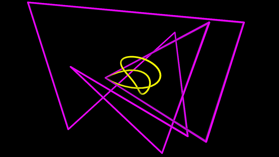
(a) Unknotted $\mathcal{L}$ with knotted $\mathcal{C}$

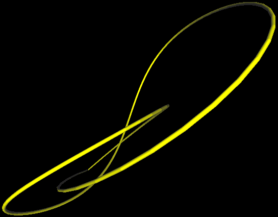
(b) Zoomed-in view of $\mathcal{C}$

Figure 1. Unknotted $\mathcal{L}$ with knotted $\mathcal{C}$

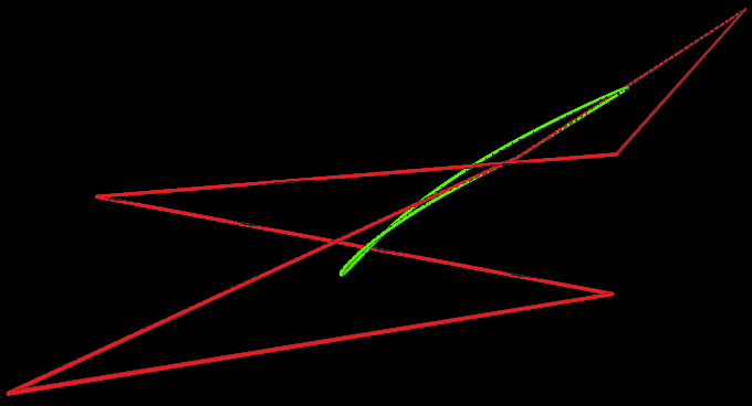
(a) Equilateral, simple $\mathcal{L}$ with self-intersecting $\mathcal{C}$

(b) Zoomed-in self-intersection

Figure 2. Equilateral, simple $\mathcal{L}$ with self-intersecting $\mathcal{C}$

1. Introduction

Computational topology lies properly within the broad scope of applied general topology and depends upon a novel integration of the ‘pure mathematics’ of topology with the ‘applied mathematics’ of numerical analysis. Computational topology also blends general topology, geometric topology and knot theory with computer visualization and graphics, as presented here. For the computational cases considered here, ideas from general topology, geometric topology and knot theory are complemented by numeric arguments in a novel integration of the ‘pure’ field of topology with the ‘applied’ focus of numerical analysis. Additionally, aspects of computer visualization and graphics are incorporated into the proofs. Much of this work was motivated by modeling biological molecules, such as proteins, as knots for visualization synchronized to simulations of the writhing of these molecules.

Attention is restricted to when $\mathcal{C}$ is closed, implying that $\mathcal{L}$ is also closed. As $\mathcal{C}$ is created from $\mathcal{L}$, it is natural to ask which topological characteristics are shared by these two curves, particularly as the control polygon often serves as an approximation to the Bézier curve in many practical applications. However, topological differences between a Bézier curve and its control polygon can exist and it is natural to develop counterexamples to show these topological differences. These counterexamples extend beyond related results, while we introduce new computational methods to generate additional counterexamples.

In Section 2, we present a counterexample of Bézier curve and its control polygon being homeomorphic, yet not ambient isotopic. To develop this counterexample, we created and used a computer visualization tool to study topological relationships between a Bézier curve and its control polygon. We viewed the images to motivate formal proofs, which also rely on numerical analysis and geometric arguments.

In Section 3, we present numerical techniques to create a class of topological counterexamples – where a Bézier curve and its control polygon are not even homeomorphic, as the Bézier curve is self-intersecting while the control polygon is simple. We exhibit self-intersection by a numerical method, which finds the roots of a system of equation. We freely admit that these roots are not determined with infinite precision, but such calculations on polynomials of degree 6, as in these examples, typically elude precise calculation. We argue that two primary values of our method for these approximated solutions are

1. as a catalyst to alternative examples that may admit infinite precision calculation and rigorous topological proofs, and

2. as having specified digits of accuracy – typically crucial for acceptable approximations in computational mathematics and computer graphics.

Using the visualization tool described in Section 4, we viewed many examples where the Bézier curve was simple, while its control polygon was equilateral and simple. It is well known that Bézier curve can be self-intersecting even when its control polygon is simple, but we conjectured that the added equilateral hypothesis would imply that both curves were simple. While this visual evidence was suggestive, we present a general numerical approach in Section 3 that supports a contrary interpretation. This example provides guidance for designing appropriate approximation algorithms for computer graphics.

1.1. Mathematical Definitions

The definitions presented are restricted to $\mathbb{R}^{3}$, as sufficient for the purposes of this paper, but the interested reader can find appropriate generalizations in published literature.

Definition 1.

A knot [4] is a curve in $\mathbb{R}^{3}$ which is homeomorphic to a circle.

Knots are often described by a knot diagram [12], which is a planar projection of a knot. Self-intersections in the knot diagram correspond to crossings in the knot, where each crossing has one arc that is an undercrossing and an overcrossing, relative to the direction of projection.

Homeomorphism is an equivalence relation over point sets and does not distinguish between different embeddings, while ambient isotopy is a stronger equivalence relation which is fundamental for classification of knots.

Definition 2.

Let $X$ and $Y$ be two subspaces of $\mathbb{R}^{3}$. A continuous function

$$H:\mathbb{R}^{3}\times[0,1]\to\mathbb{R}^{3}$$

is an ambient isotopy between $X$ and $Y$ if $H$ satisfies the following:

1. $H(\cdot,0)$ is the identity,

2. $H(X,1)=Y$, and

3. $\forall t\in[0,1],H(\cdot,t)$ is a homeomorphism from $\mathbb{R}^{3}$ onto $\mathbb{R}^{3}$.

The sets $X$ and $Y$ are then said to be ambient isotopic.

Definition 3.

Denote $\mathcal{C}(t)$ as the parameterized Bézier curve of degree $n$ with control points $P_{m}\in\mathbb{R}^{3}$, defined by

$$\mathcal{C}(t)=\sum_{i=0}^{n}{B_{i,n}(t)P_{i}},t\in[0,1]$$

where $B_{i,n}(t)=\left(\!\!\!\begin{array}[]{c}n\\ i\end{array}\!\!\!\right)t^{i}(1-t)^{n-i}$.

1.2. Related Literature

A Bézier curve and its control polygon may have substantial topological differences. It is well known that a Bézier curve and its control polygon are not necessarily homeomorphic [14]. Recently, it was shown that there exists an unknotted Bézier curve with a knotted control polygon [6]. A specific dual example has also been shown [16] of a knotted Bézier curve with an unknotted control polygon. However, the methodology was a visual construction without formal proof and is not easily generalized. Software, Knot_Spline_Vis, developed by authors Marsh and Peters, was used to find another example, where the methodology can more easily be generalized and Knot_Spline_Vis is publicly available [13].

Much of the motivation for considering these counterexamples came from applications in scientific visualization [9, 10, 11]. A primary focus was to establish tubular neighborhoods of knotted curves so that piecewise linear (PL) approximations of those curves within those neighborhoods remained ambient isotopic to the original curves. This was initially considered for approximations used in producing static images of these curves, but it became readily apparent that these same neighborhoods also provided bounds within which many perturbations of these models remained ambient isotopic under these movements. That theory is being applied to dynamic visualizations of molecular simulations, where the neighborhood boundaries permit convenient warnings as to an impending self-intersection, as of possible interest to biologists and chemists who are running the simulations.

Previous work [15] in knot visualization provides a rich set of data for PL knots, where each edge is of the same length. The interface of Knot_Spline_Vis was designed to import this equilateral PL knot data and then generate the associated Bézier curves. This matured into an empirical study of dozens of cases, where all examples examined yielded simple Bézier curves for these simple equilateral control polygons. This raised the question of whether the presence of equilateral edges in the control polygon might be a sufficient additional hypothesis to ensure homeomorphic equivalence with the Bézier curve, as the previously cited examples [14] did not have equilateral control polygons.

2. Unknotted $\mathcal{L}$ with knotted $\mathcal{C}$

In order to produce a knotted Bézier curve with an unknotted control polygon, we invoked Knot_Spline_Vis with an example (Figure 3) of an unknotted Bézier curve, where the total curvature appeared to be larger than $4\pi$. (The total curvature being larger than $4\pi$ is a necessary condition of knottedness.)

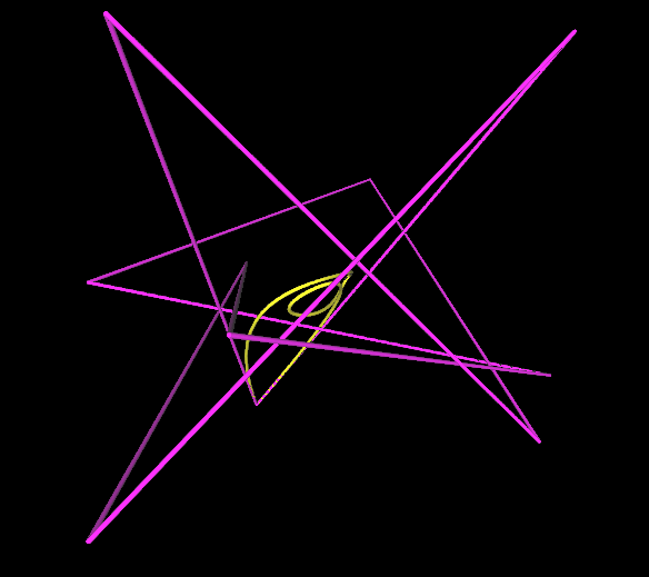
(a) Unknotted $\mathcal{C}$ & The $\mathcal{P}$

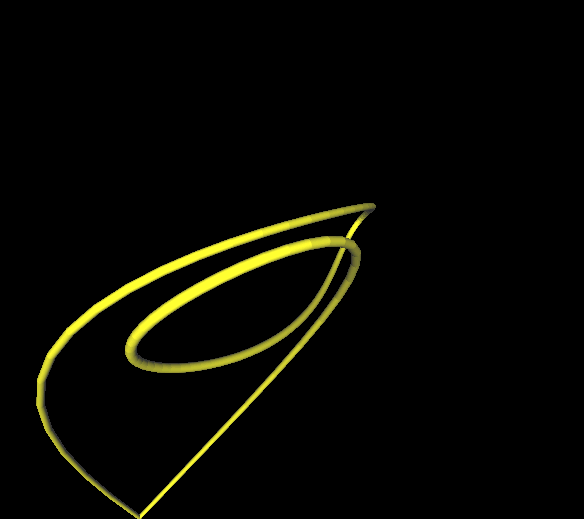
(b) Zoomed-in View of $\mathcal{C}$

Figure 3. Visual experiments

We experimented on this example by moving control points to construct a Bézier curve that visually appeared to be knotted. We then moved control points to unknot the control polygon while keeping the Bézier curve knotted. In the end we obtained a Bézier curve and the control polygon (of degree $10$) (Figure 1(a)) defined by the control points $\{P_{0},P_{1},\cdots,P_{9},P_{0}\}$ listed below:

$$(-5.9,4.7,-6.2),(10.3,-1.1,8.9),(-2.6,-12.4,-6.3),(-10,7,-0.3),$$

$$(1.9,-12,-0.6),(11.2,7.5,-7.6),(-15.3,-1.7,-4.1),(-11.7,20,3.5),$$

$$(17.9,-1.1,2.9),(2.9,-13.7,4.8),(-5.9,4.7,-6.2).$$

The 3D visualization offers only suggestive evidence that the above Bézier curve is knotted while the control polygon is unknotted. We provide rigorous mathematical proofs of these properties in Sections 2.1 and 2.2. Generally, proving knottedness or unknottedness can be difficult [8], but is accessible for the counterexample here.

2.1. Proofs of the Bézier curve being knotted

We prove that the Bézier curve is a trefoil. We orthogonally project the curve onto $x$-$y$ plane. We then shown that there are three self-intersections in the projection and these intersections are alternating crossings in 3D. Since projections preserve self-intersections, this curve can have no more than 3 self-intersections, but these self-intersections in $x$-$y$ plane are shown to have pre-images that are 3D crossings, so the original curve has no self-intersections.

Figure 4. The 2D projection of the knot

Since the 2D curve in Figure 4 has degree $10$, we use a numerical method implemented by MATLAB function ‘fminsearch’ to find the parameters where the curve intersects with itself. We provide the numerical codes in Appendix A.1, and we provide the data used to find these parameters in Appendix A.3. The pairs of parameters (labeled in order as $t_{1},\ldots,t_{6}$) of the self-intersections are listed below:

$$[t_{1}=0.0306,t_{4}=0.5573],[t_{2}=0.1573,t_{5}=0.9244],[t_{3}=0.3731,t_{6}=0.9493].$$

Next we prove that these 2D intersections are projections from three alternating crossings in 3D. The above parameters are substituted into the Bézier curve (Definition 3) to get pairs of points (numerical codes for this calculation are in Appendix A.2):

$$[\mathcal{C}(t_{1})=(-2.0539,2.8001,-2.6929),\mathcal{C}(t_{4})=(-2.0530,2.7987,-2.0143)],$$

$$[\mathcal{C}(t_{2})=(0.4376,-2.5212,-0.0576),\mathcal{C}(t_{5})=(-0.4364,-2.5206,-0.5547)],$$

$$[\mathcal{C}(t_{3})=(-1.3613,-1.4239,-2.2944),\mathcal{C}(t_{6})=(-1.3624,-1.4232,-1.9067)].$$

The alternating crossings follow from comparing the z-coordinates in each pair. Precisely, according to the parameters given above, the tracing of the six points in order is

$$\mathcal{C}(t_{1}),\mathcal{C}(t_{2}),\mathcal{C}(t_{3}),\mathcal{C}(t_{4}),\mathcal{C}(t_{5}),\mathcal{C}(t_{6}),$$

and the crossings at these points are

$$under,over,under,over,under,over.$$

2.2. Proof of the control polygon being unknotted

To prove that the control polygon $P=(P_{0},P_{1},\cdots,P_{9},P_{0})$ is an unknot, it is necessary to show that $P$ is simple and unknotted. We directly tested each pair of segments of $P$ for non-self-intersection and those calculations can be repeated by the interested reader. We prove unknottedness using a 3D push, as the obvious generalization of a 2D function from low-dimensional geometric topology [5]. We restrict attention to a median push, as defined below. The full sequence of 5 median pushes is explicated, where the first 4 median pushes are equivalently described by Reidemeister moves [12].

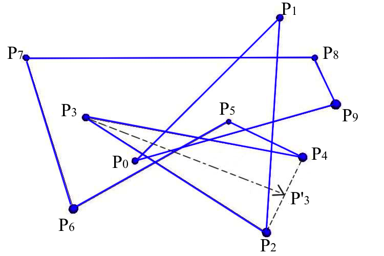
(a) The initial control polygon

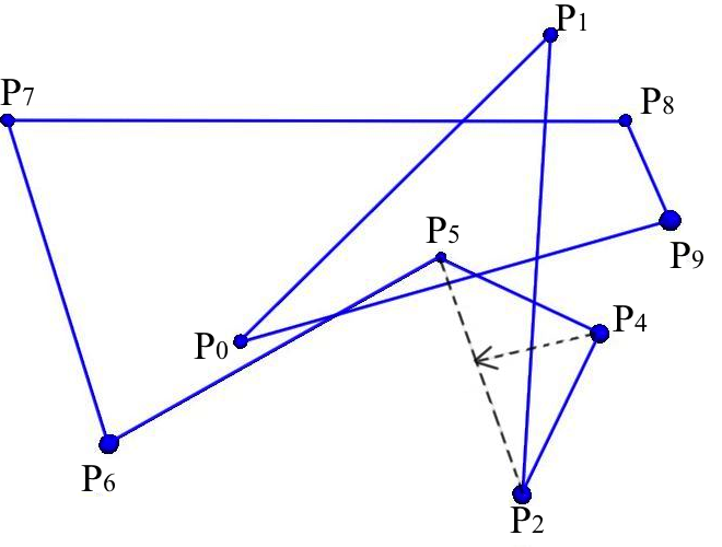
(b) After the 1st push

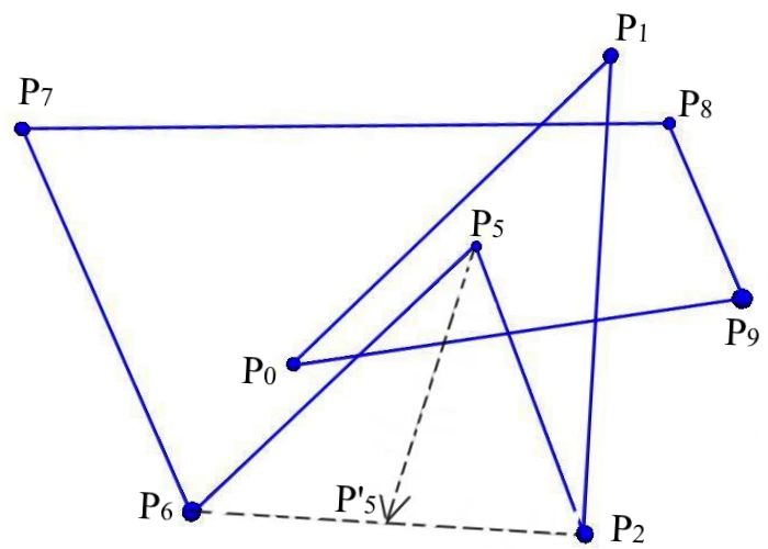
(c) After the 2nd push

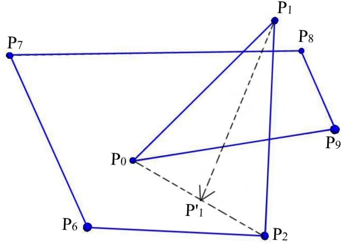
(d) After the 3rd push

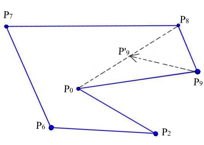
(e) After the 4th push

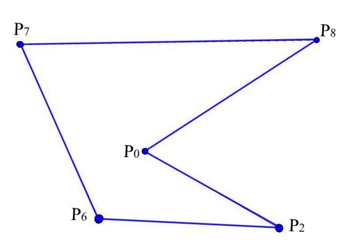
(f) The unknot after these pushes

Figure 5. Pushes and PL curves in 3D

Definition 4.

Suppose $\triangle{P_{j-1}P_{j}P_{j+1}}$ is a triangle determined by non-collinear vertices $P_{j-1},P_{j}$ and $P_{j+1}$ of $P$. Push the vertex $P_{j}$, along the corresponding median of the triangle to the middle point of the side $P_{j-1}P_{j+1}$. We call this function a median push.

We depict the sequence of pushes used in Figure 5, showing the 3D graphs of the PL space curves after the median pushes. These graphs show, at each step, which vertex is pushed and its image. For example, in Figure 5(a), the vertex $P_{3}$ is pushed to $P^{\prime}_{3}$ and the resultant polygon after this push is shown by Figure 5(b). Figures  5(a) 5(b) 5(c) and 5(d) have corresponding Reidemeister moves, as those pushes eliminate at least one crossing. Using the published notation [12], Figure 5(a) depicts a Reidemeister move of Type 2b. Similarly, Figure 5(b) depicts a Reidemeister move of Type 1b; Figure 5(c) has Type 2b and Figure 5(d) has a move of Type 2b, followed by a move of Type 1b. The final push to achieve Figure 5(f) does not correspond to any Reidemeister move as no crossings are changed, but it is included to have a polygon with only five edges, which necessarily must be the unknot [1].

We prove that $P$ is unknotted by showing that $P$ is ambient isotopic to the unknotted PL curve shown in Figure 5(f). As a sufficient condition, we show that the pushes do not cause intersections [2]. (We gained significant intuition for specifying the sequence of pushes by visual verification with our 3D graphics software capabilities to translate, rotate and zoom the images.) We now present the formal arguments.

Consider Figure 5(a), where $P_{3}$ is pushed to $P^{\prime}_{3}$ (the middle point of $\overrightarrow{P_{2}P_{4}}$). We show that any segments other than $\overrightarrow{P_{2}P_{3}}$ and $\overrightarrow{P_{3}P_{4}}$ of $P$ do not intersect the triangle $\triangle{P_{2}P_{3}P_{4}}$ or the triangle interior.

We parameterize each segment by:

$$\overrightarrow{P_{i}P_{i+1}}:P_{i}+(P_{i+1}-P_{i})t,\ t\in[0,1]$$

for $i=0,1,\cdots,9$ and let $P_{10}=P_{0}$. Then the points given by

$$P_{3}+a(P_{2}-P_{3})+b(P_{4}-P_{3}),$$

for $a,b\geq 0$ and $a+b\leq 1$ are on the $\triangle{P_{2}P_{3}P_{4}}$ and contained in its interior. Hence $P_{i}+(P_{i+1}-P_{i})t$ intersects $\triangle{P_{2}P_{3}P_{4}}$ or its interior if and only if

(1) $$P_{i}+(P_{i+1}-P_{i})t=P_{3}+a(P_{2}-P_{3})+b(P_{4}-P_{3})$$

has a solution for some $t\in[0,1]$ and $a,b\geq 0$ and $a+b\leq 1$.

For each $i=0,1,\cdots,9$, we solve Equation 1 (a system of $3$ linear equations) for $a,b$ and $t$ with the above constraints. Calculations show there is no solution for each system, and hence $P_{i}+(P_{i+1}-P_{i})t$ does not intersect $\triangle{P_{2}P_{3}P_{4}}$ or its interior for each $i=0,1,\cdots,9$. Thus it follows that the push does not cause any intersections.

Similar computations verify that the other pushes do not cause any intersections, thus establishing the ambient isotopy.

3. Equilateral, simple $\mathcal{L}$ with self-intersecting $\mathcal{C}$

We visualized many cases of simple, closed equilateral control polygons that all appeared to have unknotted Bézier curves. Many of these control polygons were nontrivial knots. Prompted by this visual evidence, we conjectured that any simple, closed equilateral control produces a simple Bézier curve, where some examples are shown in Figure 6.

We now present numerical evidence to the contrary. As noted in Section 1, the degree 6 polynomials make precise computation difficult, so we do not provide a completely formal proof, independent of numerical methods. A legitimate concern is whether the numerical approximation produces coordinates for a ‘near’ intersection, subject to the accuracy of the floating point computation. We cannot refute that possibility, but we argue that in the context of graphical images, the level of approximation produced is often sufficient. In particular, we have parameters in the code to adjust the number of digits of accuracy. This is level of user-defined precision is often accepted as sufficient for visualization [9]. The user can then set the graphical resolution so that points that are determined to be the same within some acceptable numerical tolerance will also appear within the same pixel.

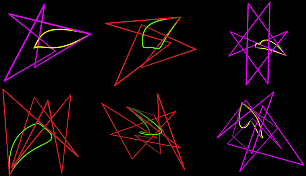
Figure 6. Unknotted Bézier curves with equilateral control polygons

3.1. Intuitive overview

We create many examples to test and retain only those that satisfy all three criteria listed in Section 3.4. We begin the creation of a closed equilateral polygon by setting $P_{0}=(0,0,0)$. We then take $\{q_{0},q_{1},\cdots,q_{n-1}\}$ (Equation 4) from the unit sphere so that

$$P_{1}=P_{0}+q_{0},\ \ \ P_{2}=P_{1}+q_{1},\ \ \ \cdots,\ \ \ P_{n}=P_{n-1}+q_{n-1}.$$

We ensure that the polygon is closed in Section 3.4 item $(3)$.

We consider a sufficient and necessary condition for a Bézier curve being self-intersecting (Equation 3). Since we want the equilateral polygon to define a Bézier curve that is self-intersecting, we not only select $\{q_{0},q_{1},\cdots,q_{n-1}\}$ from the unit sphere as above, but also select them such that Equation 3 is zero for some parameters $s$ and $t$. Consequently the set of control points generated determines a closed equilateral control polygon and a self-intersecting Bézier curve.

3.2. Necessary and sufficient condition for self-intersection

We rely upon the following published equation [3] for necessary and sufficient conditions for self-intersection of a Bézier curve

(2) $$S(s,t)=\frac{1}{n}\frac{\mathcal{C}(1-s)-\mathcal{C}(t)}{(1-s)-t},$$

with the domain $D=\{(s,t):s+t<1,s,t\geq 0,(s,t)\neq(0,0)\}$. A Bézier curve defined by $\mathcal{C}(t)$ is self-intersecting if and only if there exist $s$ and $t$ in the domain $D$ such that $S(s,t)=0$, , with an alternative formulation given by

(3) $$S(s,t)=\frac{1}{n}\sum_{i=0}^{n-1}\sum_{j=0}^{n-1-i}\binom{n-1-i}{j}s^{n-1-i-j}(1-s)^{j}\sum_{k=0}^{i}\binom{i}{k}(1-t)^{i-k}t^{k}q_{j+k},$$

where

(4) $$q_{i}=P_{i+1}-P_{i}\ \ \ \ for\ i=\{0,1,\cdots,n-1\}.$$

3.3. A representative counterexample generated

We present a single numerical counterexample, noting that while only one counterexample is presented, the numerical algorithm implemented can be used to find many such examples. We list six distinct control points (the seventh control point is equal to the first control point) that determine an equilateral simple $\mathcal{L}$ and a self-intersecting $\mathcal{C}$ (shown in Firgure 2), as generated by the algorithm described in detail in Section 3.4.

$$(0,0,0),(0.0305,0.0810,0.9962),(-0.2074,-0.2671,1.9030),$$

$$(-0.1792,-0.3402,0.9063),(0.0189,0.0782,0.0185),(0.1557,0.2329,-0.9600).$$

We verify that $\mathcal{L}$ is simple by considering all pairwise intersections of the segments of this control polygon. The self-intersection of the Bézier curve occurs at a point that is numerically approximated as

$$[s,t]=[0.2969,0.0633]$$

where correspondingly,

$$S(s,t)=(-0.0003861,-0.000097,0.0001462)\approx(0,0,0).$$

The error occurs because of numerical round off on $s,t$ and the control points.

3.4. The numerical method for generating counterexamples

We provide the numerical codes and data used in Appendix B. Given a control polygon, we can determine whether a self-intersection of the Bézier curve occurs by determining whether $S$ (Equation 3) has a root in $D$. We consider $S$ as a function $S(s,t,q)$ where $q=\{q_{i}\}_{i=0}^{n-1}$, so that finding a self-intersecting Bézier curve with an equilateral control polygon is equivalent to determining $s,t$ and $q$ such that the following are satisfied:

1. $S(s,t,q)=0$ where $s,t\in D$;

2. $||q_{i}||=r$ for each $i\in\{0,1,\cdots,n-1\}$, where $||\cdot||$ is the Euclidean norm;

3. $\sum_{i=0}^{n-1}{q_{i}}=\sum_{i=0}^{n-1}{P_{i+1}-P_{i}}=0$ since $P$ needs to be closed.

We assume $r=1$ without loss of generality since the value of $r$ can be adjusted by scaling. Throughout the provided codes, $n$ is always the degree of the Bézier curve. We give the code for function $S$ in Appendix B.1, where $[s,t]$ is labeled as $u$ and $q$ as $[a,b,c]$.

The function $SF$ (Appendix B.2) takes parameters for $s,t$ and $q$ and outputs a floating point value. It is designed to be zero if and only if the above three conditions are satisfied simultaneously.

Precisely since $q$ should be taken from the unit sphere, $SF$ assigns $a,b,c$ values given by

$$a=sin(\phi)cos(\theta);$$

$$b=sin(\phi)sin(\theta);$$

$$c=cos(\phi),$$

where $\phi$ and $\theta$ represent input parameters. In order to satisfy Condition $(3)$ above, $q_{n-1}$ is set equal to $-\sum_{i=0}^{n-2}{q_{i}}$. But in this way, $||q_{n-1}||$ may fail to be equal to $1$. So we include the function $F$ (Appendix B.2) to determine whether $||q_{n-1}||=1$. The function is designed to be $F=||q_{n-1}||-1$ such that $||q_{n-1}||=1$ if and only if $F=0$.

Symbolically,

(5) $$SF=||S||+||F||,$$

where $S$ is given by Equation 3 and $F=||q_{n-1}||-1$. Having the above three conditions satisfied simultaneously is equivalent to finding input values such that $SF=0$.

Since $SF\geq 0$, the minimum of $SF$ is $0$. The function $SFminimizer$ (Appendix B.3) uses $fminsearch$ (a numerical method integrated in MATLAB) to search for the minimum of $SF$, while returning this minimum and the corresponding values of $s,t$ and $q$. The user supplied initial guesses for $s,t$ and $q$ greatly influence the results, so we assign $SFminimizer$ randomized initial values $M$ times so that we get $M$ different minimums for different initial values. But no matter which initial values we use, as long as we can get “a” minimum of $0$, then we get the equilateral control polygon which determines a self-intersecting Bézier curve.

The data of finding the counterexample of Section 3.3 is included in Appendix B.4.

4. Visualizing Bézier curves & their control polygons

To study the knot types of a control polygon and its Bézier curve, a knot visualization tool was developed, called Knot_Spline_Vis. The tool Knot_Spline_Vis takes a PL control polygon as input and displays both the PL curve and the associated Bézier curve. For these studies, the input was always restricted to be a PL curve of known knot type. The functions of Knot_Spline_Vis were designed to permit interactive studies of the topological relationships between a Bézier curve and its control polygon. The intent is to use these examples to stimulate mathematical conjectures as a prelude to formal proofs.

Some of the standard graphical manipulation capabilities provided are illustrated in the following Figure 7 and 8, where the rotation capabilities have been particularly useful to develop visual insights into the occurrence of self-intersections and crossings as fundamental for the study of knots. An editing window allows the user to change the coordinates of the control polygons, as shown in Figure 9. The software is freely available for download at the site www.cse.uconn.edu/$\sim$tpeters.

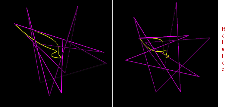
Figure 7. Rotating

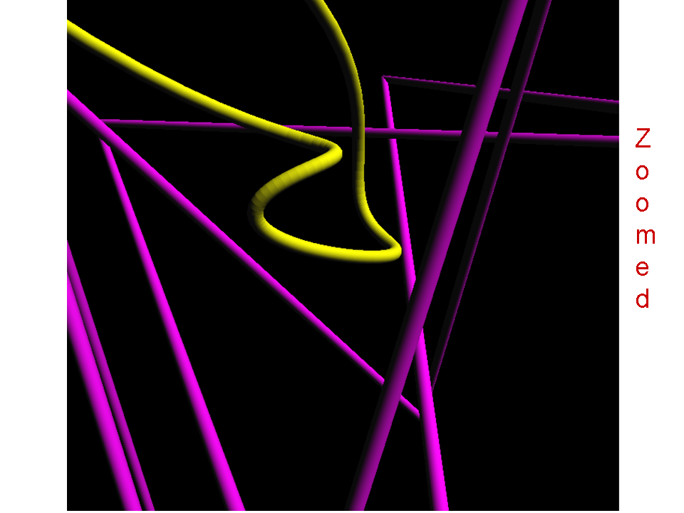
Figure 8. Scaling

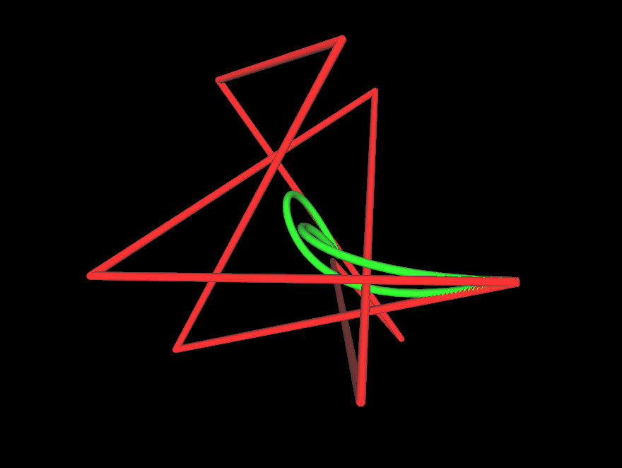
(a) Initial display

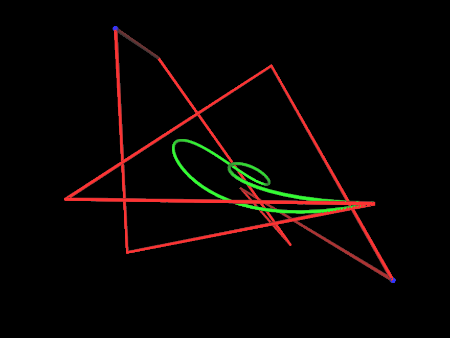
(b) Some vertices moved

Figure 9. Moving control points

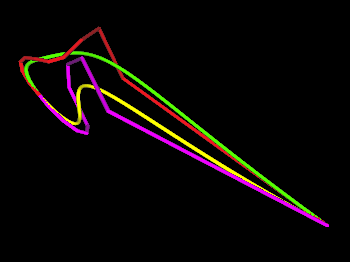
Figure 10. Subdivision

The control polygon is an initial PL approximation to its associated Bézier curve. Subdivision algorithms [14] produce additional control points to further refine the original control polygon, converging in distance to the Bézier curve. Figure 10 illustrates performance of a standard subdivision technique, the de Casteljau algorithm [7]. Users can specify a subdivision parameter. Figure 10 shows the case with parameter $\frac{1}{2}$.

5. Conclusions and Future Work

We use numerical algorithms and graphical software to generate counterexamples regarding the embeddings in $\mathbb{R}^{3}$ for a Bézier curve and its control polygon.

First, we present a class of counterexamples showing an unknotted control polygon for a knotted Bézier curve and provide complete formal proofs of this condition. We used a spline visualization tool, Knot_Spline_Vis for easy generation of many examples to gain intuitive understanding to formalize these proofs. Secondly, we used Knot_Spline_Vis in formulating the conjecture that any simple, closed equilateral control had a simple Bézier curve. We provide contrary numerical evidence regarding this conjecture, as a useful guide for many applications in computer graphics and scientific visualization.

This work also shows the importance of continuing investigation

• theoretically, into an infinite precision proof for a counterexample of the simple, closed equilateral polygon conjecture, where these demands will likely require further, substantive mathematical innovation and

• practically, into a user interface for Knot_Spline_Vis to permit interactive 3D editing, as the current text driven interface was cumbersome.

6. Web Posting of Supplemental Materials

Appendices listed below are posted on this webpage:

http://www.math.uconn.edu/~jili/Supplemental-materials.pdf

Appendix A: Numerical codes for knottedness of $\mathcal{C}$ (Figure 1(a)):

• A.1 Codes for searching self-intersections in Figure 4;

• A.2 Codes for determining under or over crossings;

• A.3 Data for searching intersections in Figure 4.

Appendix B: Numerical codes for searching the Example of Figure 2(a):

• B.1 Codes for Equation 3;

• B.2 Codes for Equation 5;

• B.3 Codes for searching the roots of the system of Equations 3 and 5;

• B.4 Data for finding the example shown in Figure 2(a).

Appendix A Code: knottedness of Bézier curve of Figure 1(a)

A.1. Code for self-intersections of Figure 4

%The function $C2d(t)$ defines the projection of the Bézier curve.
function [value] = C2d(t)
n=10;
P=zeros(2,11);
P(1,:)= [-5.9, 10.3, -2.6, -10, 1.9, 11.2, -15.3, -11.7, 17.9, 2.9, -5.9];
P(2,:)= [4.7, -1.1, -12.4, 7, -12, 7.5, -1.7, 20, -1.1, -13.7, 4.7];

sum=0;
for i=0:n
$sum=sum+nchoosek(n,i)*t^{i}*(1-t)^{(}n-i)*P(1,i+1)$;
end
$v_{1}=sum;$

sum=0;
for i=0:n
$sum=sum+nchoosek(n,i)*t^{i}*(1-t)^{(}n-i)*P(2,i+1)$;
end
$v_{2}=sum$;

$value=[v_{1},v_{2}]$;

% Use the function ‘fminsearch’ to find the minimums of $fnS(x)$, the zero minimums and parameters where the zeros occur are what we look for.

function [value] = fnS(x)
$value=norm(C2d(x(1))-C2d(x(2)),2)$;

function [value] = Smin(s0,t0)
Max=optimset(’MaxFunEvals’,1e+19);
comb=@(x)fnS(x);
u=[s0,t0];
$[xval,fval]=fminsearch(comb,u,Max)$

A.2. Code for determining crossings

%Below is the function of the Bézier curve in 3D (Definition 3).
function [value] = C(t)
n=10;
P=zeros(3,11);
P(1,:)= [-5.9, 10.3, -2.6, -10, 1.9, 11.2, -15.3, -11.7, 17.9, 2.9, -5.9];
P(2,:)= [4.7, -1.1, -12.4, 7, -12, 7.5, -1.7, 20, -1.1, -13.7, 4.7];
P(3,:)= [-6.2, 8.9, -6.3, -0.3, -0.6, -7.6, -4.1, 3.5, 2.9, 4.8, -6.2];

sum=0;
for i=0:n
$sum=sum+nchoosek(n,i)*t^{i}*(1-t)^{(}n-i)*P(1,i+1);$
end
$v_{1}=sum$;

sum=0;
for i=0:n
$sum=sum+nchoosek(n,i)*t^{i}*(1-t)^{(}n-i)*P(2,i+1);$
end
$v_{2}=sum$;

sum=0;
for i=0:n
$sum=sum+nchoosek(n,i)*t^{i}*(1-t)^{(}n-i)*P(3,i+1);$
end
$v_{3}=sum$;

$value=[v_{1},v_{2},v_{3}]$;

A.3. Data for searching intersections in Figure 4

% The Matlab commands and corresponding results:
% The initial input $(0.03,0.55)$ is figured out by the observation and calculations on self-intersections in Figure 4. Similarly for the others below.
Smin(0.03,0.55)
xval = 0.0306 0.5573
fval = 2.9567e-04

Smin(0.15,0.92)
xval = 0.1573 0.9244
fval = 1.5848e-04

Smin(0.37,0.95)
xval = 0.3731 0.9493
fval = 1.4637e-04

Appendix B Code: generating counterexamples like Figure 2(a)

B.1. Code for Equation 3

function [value] = S(u,a,b,c)
sum=0; subsum1=0; subsum2=0;
for i=0:n-1
for j=0:n-1-i
% The use of adding $1$ to the vectors $a,b$ and $c$ is required by MATLAB.
for k=0:i $subsum2=subsum2+nchoosek(i,k)*(1-u(2))^{(i-k)}*u(2)^{k}*a(j+k+1);$
end
$subsum1=subsum1+subsum2*nchoosek(n-1-i,j)*u(1)^{(n-1-i-j)}*(1-u(1))^{j};$
end
$sum=sum+subsum1;$
end
$v_{1}=(1/n)*sum;$

sum=0; subsum1=0; subsum2=0;
for i=0:n-1
for j=0:n-1-i
for k=0: i
$subsum2=subsum2+nchoosek(i,k)*(1-u(2))^{(i-k)}*u(2)^{k}*b(j+k+1);$
end
$subsum1=subsum1+subsum2*nchoosek(n-1-i,j)*u(1)^{(n-1-i-j)}*(1-u(1))^{j};$
end
$sum=sum+subsum1;$
end
$v_{2}=(1/n)*sum;$

sum=0; subsum1=0; subsum2=0;
for i=0:n-1
for j=0:n-1-i
for k=0:i $subsum2=subsum2+nchoosek(i,k)*(1-u(2))^{(i-k)}*u(2)^{k}*c(j+k+1);$
end
$subsum1=subsum1+subsum2*nchoosek(n-1-i,j)*u(1)^{(n-1-i-j)}*(1-u(1))^{j};$
end
$sum=sum+subsum1;$
end
$v_{3}=(1/n)*sum;$
$value=[v_{1},v_{2},v_{3}];$

B.2. Code for Equation 5

function [value] = SF(x,n)
q=zeros(3,n); p=zeros(3,n+1);
a=zeros(1,n);b=zeros(1,n);c=zeros(1,n);
$alpha=zeros(1,2*n-2);$
for $i=1:2*n-2$
alpha(i)=x(i);
end
for i=1:n-1
$a(i)=sin(alpha(i))*cos(alpha(n-1+i));\\ b(i)=sin(alpha(i))*sin(alpha(n-1+i));\\ c(i)=cos(alpha(i));$
q(:,i)=[a(i),b(i),c(i)];
end

a(n)=0; b(n)=0; c(n)=0;
for i=1:n-1
a(n)=a(n)-a(i); b(n)=b(n)-b(i); c(n)=c(n)-c(i);
q(:,n)=[a(n),b(n),c(n)];
end

u=zeros(1,2); $u=[x(2*n-1),x(2*n)];$
value=abs(F(alpha,n))+norm(S(u,a,b,c),2);

for i=1:n
for j=1:i;
p(:,i+1)=p(:,i+1)+q(:,j);
end
end
p


function [value]=F(alpha,n)
for i=1:n-1
$a(i)=sin(alpha(i))*cos(alpha(n-1+i));b(i)=sin(alpha(i))*sin(alpha(n-1+i));c(i)=cos(alpha(i));$
end

a(n)=0; b(n)=0; c(n)=0;
for i=1:n-1
a(n)=a(n)-a(i); b(n)=b(n)-b(i); c(n)=c(n)-c(i);
end
$value=abs(a(n)^{2}+b(n)^{2}+c(n)^{2}-1);$

B.3. Codes for solving the system of Equations 3 and 5

function [value] = SFminimizer(n,M)
Max=optimset(ḾaxFunEvals,́1e+9);
comb=@(x)SF(x,n);
xval=zeros(2*n,M);
fval=zeros(1,M);

for i=1:M
phi=unifrnd(0,pi,1,n-1); theta=unifrnd(0,2*pi,1,n-1);
s0=unifrnd(0,1); t0=unifrnd(0,1-s0);
x0=[phi,theta,s0,t0];
$[xval(:,i),fval(i)]=fminsearch(comb,x0,Max);$
%make sure $s+t=xval(2*n-1,i)+xval(2*n,i)<1$ so that $s,t\in D$.
$if\ xval(2*n-1,i)+xval(2*n,i)>1\ or\ xval(2*n-1,i)+xval(2*n,i)=1$
fval(i)=1;
else
end
end

%Display the minimums and corresponding $s,t$ and $q$.
xval fval
%Returns the optimal one.
$[C,I]=min(fval);$
value=[C,I];

B.4. Data for finding the example shown in Figure 2(a)

The counterexample (Section 3.3) uses the second column below for the input parameters.
SFminimizer(6,10)
xval =
Columns 1 through 10
2.1907 0.0867 1.0279 2.4529 0.8294 1.3029 1.0958 0.8502 1.2136 0.3308
2.1572 0.4353 1.9303 0.3841 -0.2788 0.3006 -0.2769 2.8797 3.0782 3.1699
0.0079 3.2225 3.2107 1.8739 3.1482 3.6489 1.3900 0.5959 0.1228 1.8107
0.5496 2.6633 0.2000 1.1955 0.5784 2.0316 1.6273 2.0583 3.1341 1.3276
1.8511 2.9336 1.0424 2.6615 2.3439 1.2207 2.4580 4.3850 0.1877 -0.1146
5.2200 1.2107 7.0598 3.4826 0.3696 0.5633 5.1432 4.2546 3.5523 5.5103
2.7090 4.1128 4.1941 2.3445 2.4291 2.0589 0.4295 2.9467 1.0576 5.9281
0.1954 2.0119 2.2644 7.0575 2.1168 2.3027 1.9744 -0.2264 2.5206 2.4902
0.5312 7.4240 2.2923 5.1205 1.2132 4.0211 3.4493 1.6729 1.7930 5.7145
1.3429 0.8465 1.4447 4.4661 4.0120 1.8860 0.0947 3.9222 5.1409 1.2114
0.5200 0.2969 0.7942 0.7334 0.2149 0.6042 1.3269 0.9360 0.1185 0.0320
0.0054 0.0633 0.2813 0.2543 0.6229 0.4588 0.0165 0.1667 0.5815 0.5970

fval =
Columns 1 through 7
0.0000 0.0000 1.0000 0.2180 0.0001 1.0000 1.0000
Columns 8 through 10
1.0000 0.0001 0.0000

% The corresponding function values of $S$ and $F$ are given:
Svalue = $1.0e-03*$
-0.3861 -0.0970 0.1462

Fvalue =$2.2329e-05$

References

- [1] C.C. Adams. The Knot Book: An Elementary Introduction To The Mathematical Theory Of Knots. American Mathematical Society, 2004.
- [2] J. W. Alexander and G. B. Briggs. On types of knotted curves. Annals of Mathematics, 28:562–586, 1926-1927.
- [3] L. E. Andersson, T. J. Peters, and N. F. Stewart. Selfintersection of composite curves and surfaces. CAGD, 15:507–527, 1998.
- [4] M. A. Armstrong. Basic Topology. Springer, New York, 1983.
- [5] R. H. Bing. The Geometric Topology of 3-Manifolds. American Mathematical Society, Providence, RI, 1983.
- [6] J. Bisceglio, T. J. Peters, J. A. Roulier, and C. H. Sequin. Unknots with highly knotted control polygons. CAGD, 28(3):212–214, 2011.
- [7] G. Farin. Curves and Surfaces for Computer Aided Geometric Design. Academic Press, San Diego, CA, 1990.
- [8] J. Hass, J. C. Lagarias, and N. Pippenger. The computational complexity of knot and link problems. Journal of the ACM, 46(2):185–221, 1999.
- [9] K. E. Jordan, R. M. Kirby, C. Silva, and T. J. Peters. Through a new looking glass*: Mathematically precise visualization. SIAM News, 43(5):1– 3, 2010.
- [10] K. E. Jordan, L. E. Miller, E. L. F. Moore, T. J. Peters, and A. C. Russell. Modeling time and topology for animation and visualization with examples on parametric geometry. Theoretical Computer Science, 405:41–49, 2008.
- [11] K. E. Jordan, L. E. Miller, T. J. Peters, and A. C. Russell. Geometric topology and visualizing 1-manifolds. In V. Pascucci, X. Tricoche, H. Hagen, and J. Tierny, editors, Topology-based Methods in Visualization, pages 1 – 12, New York, 2011. Springer.
- [12] C. Livingston. Knot Theory, volume 24 of Carus Mathematical Monographs. Mathematical Association of America, Washington, DC, 1993.
- [13] T. J. Peters and D. Marsh. Personal home page of T. J. Peters. http://www.cse.uconn.edu/.
- [14] L. Piegl and W. Tiller. The NURBS Book. Springer, New York, 2nd edition, 1997.
- [15] R. Scharein. The knotplot site. http://www.knotplot.com/.
- [16] C. H. Sequin. Spline knots and their control polygons with differing knottedness. http://www.eecs.berkeley.edu/Pubs/TechRpts/2009/EECS-2009-152.html.