Waves in the Skyrme–Faddeev model and integrable reductions

Abstract

In the present article we show that the Skyrme–Faddeev model possesses nonlinear wave solutions, which can be expressed in terms of elliptic functions. The Whitham averaging method has been exploited in order to describe slow deformation of periodic wave states, leading to a quasi-linear system. The reduction to general hydrodynamic systems have been considered and it is compared with other integrable reductions of the system.

1 Introduction

The main aim of the present paper is to study periodic and multi-periodic solutions of the so-called Skyrme–Faddeev model. In the recent years a special interest was deserved by the 3D static nonlinear Skyrme – Faddeev $\sigma$-model for the field ${\bm{\phi}}:\mathbb{R}^{3}\rightarrow\mathbb{S}^{2}$, the total free energy of which is given by

$$S_{SF}=\int d^{3}x\left[\frac{1}{4}\rho^{2}\left(\partial_{k}{{\bm{\phi}}}\right)^{2}+H_{ik}^{2}\right],\quad\left\{\begin{array}[]{ll}H_{ik}={\bm{\phi}}\cdot\left[\partial_{i}{\bm{\phi}}\times\partial_{k}{\bm{\phi}}\right],&\\ {\bm{\phi}}\cdot{\bm{\phi}}=1,&\end{array}\right.$$ (1.1)

where $\rho$ is a real positive constant and $H_{ik}$ is an antisymmetric tensor field, the so-called Mermin - Ho vorticity [1, 2, 3] in Matter Physics, expressing the non irrotational properties of the multi-component superfluid. On the other hand, after a long work [4, 5], it was proved that (1.1) can be seen as a special subcase, among many others [6], for the background (classical) field of the quantum pure $SU\left(2\right)$-Yang-Mills theory in the infrared limit, thus describing a self-consistent “mesonic” field in the context of the Nuclear Physics.

The main interest is to look for localized finite energy solutions, for which one imposes a constant value at spatial infinity, for instance $\lim_{\left|\mathbf{x}\right|\rightarrow\infty}{{\bm{\phi}}}=\left(0,0,1\right)$, compactifying to $\mathbb{S}^{3}$ the space domain. Then, from the homotopy group theory result $\pi_{3}\left(\mathbb{S}^{2}\right)={\mathbb{Z}}$ [7], one can conclude that all such solutions (hopfions) are labelled by the so-called Hopf index $Q$ into separated sectors. The Hopf index can be computed analytically, since $H_{ik}$ in the expression (1.1) is a closed 2-form on $\mathbb{S}^{3}$, so derivable from a 1-form $a_{k}=-\frac{\varepsilon_{ijk}}{4\pi}\int_{S^{3}}\frac{\left(x_{i}-x_{i}^{\prime}\right)H_{ij}\left(x^{\prime}\right)}{\left[\left(x_{m}-x_{m}^{\prime}\right)^{2}\right]^{3/2}}d^{3}x^{\prime}$. Thus one has [8, 9, 10]

$$Q=\frac{1}{16\pi^{2}}\int d^{3}x\,\varepsilon_{ikl}a_{i}\partial_{k}a_{l},$$

expressing the linking number of the pre-images of two independent points on the target $\mathbb{S}^{2}$, then $Q=0$ for spherical solutions, 1 for toroidal shaped vortices. Only approximated analytical solutions are known [11]. Many times tangled hopfions have been confirmed by numerical studies [12, 13, 14, 15, 16], which have produced a comprehensive analysis of solitons with $1\leq Q\leq 16$, proving the existence of local energy minima with knotted structure. On the other hand, global analytical considerations [8, 9, 10, 17] have shown that the energy of such a knot is bounded from below by $S_{SF}\geq C\;\pi^{2}\;\rho\;|Q|^{3/4}$, where $C$ is a constant evaluated numerically [16]. The main consequence of the above bound is that hopfions of higher topological charge can be broken only by adding an extra energy contribution for their disentanglement. However, also space extended structures were considered in [18] and in [19]. In the latter it was shown that periodic collection of localized objects may condensate in order to form periodic structure in the space. However, as pointed out in [19] the appearance of extended multi-sheeted structures, similar in some extent to the stripes found in [18], may be energetically more favorable. Thus, the quest for periodic (possibly exact) solutions for the Skyrme–Faddeev model becomes more interesting. On the other hand, in a series of papers [20], it was shown that, by adding certain differential constraints to the equation of motion of the Lorentz invariant version of (1.1), one may obtain completely integrable sub systems, with infinitely many local conservation laws. This was another hint in the direction of integrable reductions. On the experience of the hydrodynamic reductions we tried different approaches, which lead us to identify 1) quasi-periodic solutions described in terms of elliptic integrals, 2) the average motion of periodic waves accordingly to Whitham’s method, 3) constraints on the solutions expressed in terms of several Riemann invariants. The paper is organized into an Introduction and three further Sections, concerning the previously listed topics and final considerations are included in Conclusions.

2 Periodic Solution

First we consider the Skyrme–Faddeev model in the 4-dimensional relativistic space time [9], defined on the space-time $M=\left\{\left(x^{0},\ldots,x^{3}\right)\right\}$ endowed with the (pseudo)-Riemannian metric $\text{diag}\left(g_{\mu}\right)=\left(+,-,-,-\right)$, given by the Lagrangian density

$$\mathcal{L}=\frac{1}{32\pi^{2}}\;\left({\partial}_{\mu}{\bm{\phi}}\cdot\partial^{\mu}{\bm{\phi}}-\frac{\lambda}{4}\left(\partial_{\mu}{\bm{\phi}}\times\partial_{\nu}{\bm{\phi}}\right)\cdot\left(\partial^{\mu}{\bm{\phi}}\times\partial^{\nu}{\bm{\phi}}\right)\right)-\kappa\left(1-{\bm{\phi}}\cdot{\bm{\phi}}\right),$$ (2.2)

where $\lambda=\frac{16}{\rho^{2}}>0$ is the scaling parameter describing the breaking of the conformal symmetry and $\kappa$ is a Lagrangian multiplier implementing the constraint ${\bm{\phi}}\in\emph{S}^{2}$. The model (1.1) is obtained by setting ${\partial}_{0}{\bm{\phi}}\equiv 0$.

It is well known that the geometric constraint ${\bm{\phi}}\cdot{\bm{\phi}}=1$ can be realized in several ways, but here it seems useful to introduce the polar representation

$${\bm{\phi}}=\left(\sin\widetilde{\Theta}\sin\widetilde{\Phi},\sin\widetilde{\Theta}\cos\widetilde{\Phi},\cos\widetilde{\Theta}\right),$$ (2.3)

where $\widetilde{\Theta}$ and $\widetilde{\Phi}$ are suitable function on the variables $\left(x^{0},\ldots,x^{3}\right)$ to be determined. The Lagrangian (2.2) becomes

$$\mathcal{L}_{p}=\frac{1}{32\pi^{2}}\;\left\{\widetilde{\Theta}_{\mu}\widetilde{\Theta}^{\mu}+\sin^{2}\widetilde{\Theta}\left[\widetilde{\Phi}_{\mu}\widetilde{\Phi}^{\mu}-\frac{\lambda}{2}\left(\widetilde{\Theta}_{\mu}\widetilde{\Theta}^{\mu}\widetilde{\Phi}_{\nu}\widetilde{\Phi}^{\nu}-\widetilde{\Theta}_{\mu}\widetilde{\Theta}_{\nu}\widetilde{\Phi}^{\mu}\widetilde{\Phi}^{\nu}\right)\right]\right\}.$$ (2.4)

Now, it is well known [11] that the equations of motion given by (1.1) admit harmonic plane wave solutions of the of the form

$${\bm{\phi}}=\left(\frac{2A\cos\left(p_{i}x^{i}\right)}{A^{2}+1},\frac{2A\sin\left(p_{i}x^{i}\right)}{A^{2}+1},\frac{1-A^{2}}{A^{2}+1}\right),$$ (2.5)

where $A$ parameterizes the amplitude of the third component and remarkably the dispersion law is given by $p_{i}p^{i}=0$ . Actually, by using the symmetry group of the model one can find a 12 parametric family (4 translations, 4 boosts/rotations and 3 gauge transformations) of solutions. In particular, the axis of precession can be arbitrarily fixed by gauge transformations. Nevertheless, they cannot be superimposed, because of the nonlinearity character of the equations of motion. To have a visualization of (2.5) can think to a periodic assembly of vectors, whose wave front are orthogonal to the direction ${\bm{p}}=\left(p_{1},p_{2},p_{3}\right)$, and maintaining constant the projection $\phi_{3}$. The configuration is similar to a cholesteric liquid crystal. Moreover the energy density of the configuration is constant in the whole space, being equal to $\mathcal{E}=\frac{A^{2}{\bm{p}}^{2}}{4\pi^{2}\left(1+A^{2}\right)^{2}}$. Notice how solutions with smaller third component are more energetic.

Looking for the simplest generalization of (2.5), one assumes that

$$\widetilde{\Theta}=\Theta\left[\theta\right],\text{ }\widetilde{\Phi}=\Phi\left[\theta\right]+\tilde{\theta},\text{ where \ }\theta=\alpha_{\mu}x^{\mu},\tilde{\theta}=\beta_{\mu}x^{\mu}$$ (2.6)

in which one distinguishes $\theta$ as the phase from the pseudo-phase $\tilde{\theta}$. From a different point of view, we are looking for invariant solutions under a 8-parametric family of 2-dimensional Abelian sub-algebra of the translation symmetry group given by

$$\left\{{\bm{v}}_{\alpha}=\sum_{i=1}^{3}\alpha_{i}\mathbf{t}_{0}-\alpha_{0}\sum_{i=1}^{3}\mathbf{t}_{i},{\bm{v}}_{\beta}=\sum_{i=1}^{3}\beta_{i}\mathbf{t}_{0}-\beta_{0}\sum_{i=1}^{3}\mathbf{t}_{i}\right\},$$ (2.7)

where $\mathbf{t}_{i}$’s are the generators of the translations. Actually, by using the adjoint action of the space-time rotational subgroup, we can conjugate each of the above subalgebras to exactly one representative sub-algebra of the form (2.7) belonging to a 3-parametric sub-family. However, it is more easy to deal with all components for notational homogeneity. Thus the equations of motion reduce to the announced 3-parametric family

$$\left[2B_{3}-\frac{\lambda}{4}\mathcal{B}\sin^{2}\Theta\right]\Theta_{\theta\theta}=\sin 2\Theta\left(\frac{\lambda}{8}\mathcal{B}\;\Theta_{\theta}^{2}+B_{3}\Phi_{\theta}^{2}+B_{2}\Phi_{\theta}+B_{1}\right)$$ (2.8)

$$2B_{3}\sin^{2}\Theta\;\Phi_{\theta\theta}+\Theta_{\theta}\sin 2\Theta\left(2B_{3}\Phi_{\theta}+B_{2}\right)=0,$$ (2.9)

where $B_{1}=-\beta_{\mu}\beta^{\mu}$, $B_{2}=-2\alpha_{\mu}\beta^{\mu}$ $B_{3}=-\alpha_{\mu}\alpha^{\mu}$ and $\mathcal{B}=B_{2}^{2}-4B_{1}B_{3}$.

Of course these equations provide the above linear solutions (2.5), setting $B_{3}=0$ and $B_{2}\neq 0$, then $\Theta=2\arctan A$, $\Phi=\Phi_{0}-\frac{B_{1}}{B_{2}}\theta$ and $p_{i}=\frac{B_{2}\beta_{i}-B_{1}\alpha_{i}}{B_{2}}$. On the other hand, for $B_{3}\neq 0$, the solution is given by $\Theta=2\arctan A$ and $\Phi=\Phi_{0}-\frac{B_{2}\pm\sqrt{\mathcal{B}}}{2B_{3}}\theta$, with an analogous expression for the $p_{i}$’s.

To deal with the general situation one uses the expression of the energy-stress tensor $T^{\mu\nu}=\left(\widetilde{\Theta}^{\nu}{\partial}_{\widetilde{\Theta}_{\mu}}+\widetilde{\Phi}^{\nu}{\partial}_{\widetilde{\Phi}_{\mu}}\right)\mathcal{L}_{P}-g^{\mu\nu}\mathcal{L}_{P}$. Substituting in it the ansatz (2.3), only derivatives with respect to $\theta$ survive. Thus, the further vanishing divergence is equivalent to take ${\partial}_{\theta}$ over a quantity obtained by contracting $\mathcal{E}^{\mu}=T^{\mu\nu}\alpha_{\nu}$, corresponding to total conserved quantities for the wave, seen as a function of the phase. Their expressions are

$$\mathcal{E}^{0} = \frac{-1}{32\pi^{2}}\left\{B_{3}\alpha_{0}\Theta_{\theta}^{2}+\sin^{2}\Theta\left[2{\bm{\alpha}}\cdot{\bm{\beta}}\,\beta_{0}+\left(B_{1}-2{\bm{\beta}}^{2}\right)\alpha_{0}\right.\right.$$ (2.10)

$$\left.\left.+B_{3}\left(2\beta_{0}+\alpha_{0}\Phi_{\theta}\right)\Phi_{\theta}-\frac{\lambda\mathcal{B}}{8}\alpha_{0}\Theta_{\theta}^{2}\right]\right\},$$

$$\ \mathcal{E}^{i} = \frac{-1}{32\pi^{2}}\left\{B_{3}\alpha_{i}\Theta_{\theta}^{2}+\sin^{2}\Theta\left[B_{2}\beta_{i}-B_{1}\alpha_{i}+B_{3}\left(2\beta_{i}+\alpha_{i}\Phi_{\theta}\right)\Phi_{\theta}-\frac{\lambda\mathcal{B}}{8}\alpha_{i}\Theta_{\theta}^{2}\right]\right\}.$$

These equations can be used to find an expression of $\Theta_{\theta}^{2}$ and $\Phi_{\theta}$. Precisely, assuming $B_{3}\neq 0$ one finds

$$\Theta_{\theta}^{2} = \frac{8B_{3}\left(B_{1}\sin^{2}\Theta+U_{3}\right)-2B_{2}^{2}\left(\sin^{2}\Theta+U_{2}^{2}\csc^{2}\Theta\right)}{B_{3}\left(8B_{3}-\lambda\mathcal{B}\sin^{2}\Theta\right)},$$ (2.11)

$$\Phi_{\theta} = -\frac{B_{2}\left(U_{2}\csc^{2}(\Theta)+1\right)}{2B_{3}},$$ (2.12)

where the $U_{i}$’s are two constants completely defining the quantities in (2.10) by the expressions $\mathcal{E}^{\mu}=U_{3}\alpha_{\mu}+\frac{B_{2}U_{2}}{2}\left(\frac{B_{2}}{B_{3}}\alpha_{\mu}-2\beta_{\mu}\right)$. Thus, one has reduced the problem to the quadratures, introducing only two new integration constants besides $\left\{U_{2},U_{3}\right\}$, which determine the amplitudes of the phases. Finally similar conclusions can be obtained in the case $B_{3}=0$. Despite of its involved expression, equation (2.11) can be set in algebraic form by the transformation

$$\Theta=\arcsin\sqrt{\psi},$$ (2.13)

forcing to be $0\leq\psi\leq 1$ and to be satisfied the equation

$$\psi_{\theta}^{2}=\frac{64(\psi-1)\left(\psi-A_{1}\right)\left(\psi-A_{2}\right)}{\lambda^{2}\mathcal{B}\psi_{1}\left(\psi_{1}-\psi\right)},$$ (2.14)

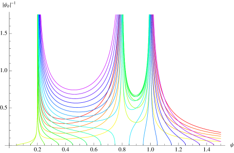
Figure 1: The graphic for the inverse square root of (2.14) for the family of parameters $\mathcal{B}=1,A_{1}=.1,A_{2}=.8$ and $-.45\leq\psi_{1}\leq 1.55$ with steps of 0.1. Colors run accordingly from red to violet. Only one bounded periodic solutions exists for any set of parameters. The degenerate case $\psi_{1}=A_{2}=.8$ is not considered, but it corresponds to the confluence of the two yellow curves.

where one has defined the constants $A_{1,2}=\frac{2B_{3}U_{3}\pm\sqrt{4B_{3}^{2}U_{3}^{2}-\mathcal{B}\,U_{2}^{2}}}{\mathcal{B}}$, related 1-1 to the values of the integrals of motion, and $\psi_{1}=\frac{8B_{3}}{\lambda\mathcal{B}}$. Assuming $A_{i}$ to be real and setting $0<A_{1}<A_{2}<1$ for instance, by a continuous variation of $\psi_{1}$ one obtains different behaviors of oscillation amplitudes for $\psi$: $A_{2}<\psi<1$ for $\psi_{1}<0$, $A_{1}<\psi<A_{2}$ for $0<\psi_{1}<A_{2}$, $A_{1}<\psi<1$ for $\psi_{1}=A_{2}$, $A_{2}<\psi<1$ for $A_{2}<\psi_{1}$. So for all choices of $\psi_{1}$ there is only one oscillating solution, bounded between two of the three zeros of the numerator in (2.14), even if real unbounded solution may appear or complex ones (see Figure 1).

Analytically, equation (2.14) can be integrated in terms of incomplete elliptic integrals of the third kind. Precisely, by introducing a parametric variable $Z$ one obtains the parametric form

$$\theta\left(\psi\right) = \theta_{0}+\frac{1}{4}\sqrt{\frac{\mathcal{B}\lambda^{2}\psi_{1}\left(\psi_{1}-A_{1}\right)^{2}}{\left(A_{1}-1\right)\left(A_{2}-\psi_{1}\right)}}\Pi\left[\frac{A_{1}-A_{2}}{\psi_{1}-A_{2}};Z|\frac{(\psi_{1}-1)\left(A_{1}-A_{2}\right)}{\left(A_{1}-1\right)\left(\psi_{1}-A_{2}\right)}\right],$$

$$\psi = -\frac{A_{2}\psi_{1}\sin^{2}Z+A_{1}\left(\psi_{1}\cos^{2}Z-A_{2}\right)}{A_{1}\sin^{2}Z+A_{2}\cos^{2}Z+\psi_{1}}$$ (2.15)

which can be expressed in terms of Weierstrass $\mathcal{P}$ function. Furthermore, from (2.12) the function $\Phi$ can be expressed again in terms of incomplete elliptic integrals, namely

$$\Phi = -\frac{B_{2}U_{2}}{2B_{3}}\left[\int\frac{d\theta}{\psi\left(\theta\right)}+\theta\right]+\Phi_{0}=$$

$$- \frac{s_{1}}{2\psi_{1}}\left[\sqrt{\frac{2\psi_{1}\left(A_{1}-\psi_{1}\right){}^{2}\left(B_{1}\lambda\psi_{1}+2\right)}{\left(A_{1}-1\right)\left(A_{2}-\psi_{1}\right)}}\Pi\left(\frac{A_{2}-A_{1}}{A_{2}-\psi_{1}};Z\left|\frac{\left(A_{1}-A_{2}\right)\left(\psi_{1}-1\right)}{\left(A_{1}-1\right)\left(\psi_{1}-A_{2}\right)}\right.\right)\right.$$

$$\left.+2s_{2}\sqrt{\frac{A_{2}\psi_{1}\left(A_{1}-\psi_{1}\right){}^{2}}{A_{1}\left(A_{1}-1\right)\left(A_{2}-\psi_{1}\right)}}\Pi\left(\frac{\left(A_{1}-A_{2}\right)\psi_{1}}{A_{1}\left(\psi_{1}-A_{2}\right)};Z\left|\frac{\left(A_{1}-A_{2}\right)\left(\psi_{1}-1\right)}{\left(A_{1}-1\right)\left(\psi_{1}-A_{2}\right)}\right.\right)\right],$$

where $s_{1}=\text{sign\thinspace}B_{2}$, $s_{2}=\text{sign \thinspace}U_{2}$

In this parametric form it is evident that the phases of the spinorial field and the phase $\theta$ do not have the same periodicity. Thus the solution is generically quasi periodic and only for very special choices of the parameters true periodic solutions appear (see Figure 4 ). Then it is convenient to adopt, as we will show in the next section, a method which allows to describe solutions with a minimal set of parameters, concerning only the periodicity in the phase. Here notice only that the length-wave can be made very large when $A_{2}\rightarrow 1$ and $\psi_{1}\rightarrow\infty$.

Then, an important observation occurs now: one has found a special 2-dimensional reduction of the Skyrme–Faddeev model, which is completely integrable, and one may wonder if this is not in the class described in [20]. If one performs the transformation of the polar representation of the field $\phi$ into the stereographic projection

$$w=i\tan\left(\frac{\Theta}{2}\right)\exp\left(-i\tilde{\Phi}\right),w^{\ast}\rightarrow-i\tan\left(\frac{\Theta}{2}\right)\exp\left(i\tilde{\Phi}\right),$$ (2.17)

the constraint imposed by the authors in [20] is expressed by

$${\partial}_{\mu}w\;{\partial}^{\mu}w=0.$$ (2.18)

One easily verifies that it is satisfied by the harmonic wave solution (2.5). On the other hand, if one replaces in (2.18) the reduction in (2.6), depending on phase and pseudo-phase, one obtains the relation

$$\sin^{2}(\Theta)\left(\Phi_{\theta}\left(B_{3}\Phi_{\theta}+B_{2}\right)+B_{1}\right)-B_{3}\Theta_{\theta}^{2}+$$

$$i\,\sin(\Theta)\left(2B_{3}\Phi_{\theta}+B_{2}\right)\Theta_{\theta}=0$$ (2.19)

from which one sees that separately real and imaginary parts have to vanish. Replacing the condition (2.12) into the last equation, one obtains

$$-B_{3}\Theta_{\theta}^{2}+B_{1}\sin^{2}(\Theta)-iB_{2}U_{2}\Theta_{\theta}\csc(\Theta)-\frac{B_{2}^{2}\left(\sin^{2}(\Theta)-U_{2}^{2}\csc^{2}(\Theta)\right)}{4B_{3}}=0,$$ (2.20)

saying that, excluding constant $\Theta$ solutions, or $B_{2}$ or $U_{2}$ have to be zero. But compatibility with equation (2.11) implies the constancy of $\Theta$ in both cases. So, in conclusion, the solutions found above are out of the sub-sector described by the constraint (2.18).

In the next Section we average the periodic solutions of the Skyrme–Faddeev model by the Whitham approach.

3 The Whitham averaging method

The Whitham approach was developed for any multi-dimensional system possessing a Lagrangian formulation (see details in [21]). Nevertheless, only some year later, the first averaging on a multi-dimensional example, the well known three dimensional Kadomtsev-Petviashvili equation, was provided by E. Infeld [22]. Now, more than thirty years later, we present the second multi-dimensional example, i.e. we are considering the averaging of the four dimensional Skyrme–Faddeev model. As we have seen above, this nonlinear system is determined by a Lagrangian (see (2.2) and (2.4)) and possesses a multi-parametric family of periodic solutions (2.14) (see also (2.11) and (2.12)). In such a case, following a heuristic approach, one can introduce the averaged Lagrangian $L(\gamma,\omega,\bm{\beta},\bm{k})$ in the new dynamical variables $\gamma,\omega,\bm{\beta},\bm{k}$, which correspond to the derivatives with respect to space time variables of phase $\theta$ and pseudo-phase $\tilde{\theta}$, now not necessarily linear as in (2.6). It means that $\omega=-\theta_{x^{0}},k^{i}=\theta_{x^{i}}$ and $\gamma=-\tilde{\theta}_{x^{0}},\beta^{i}=\tilde{\theta}_{x^{i}}$. Thus, one immediately derives the four-dimensional quasilinear system

$$\partial_{x^{0}}L_{\omega}=\partial_{x^{i}}L_{k^{i}},\text{ \ \ }\partial_{x^{0}}L_{\gamma}=\partial_{x^{i}}L_{\beta^{i}},$$ (3.21)

with the compatibility conditions

$$k_{x^{0}}^{1}+\omega_{x^{i}}=0,\text{ \ \ },\text{ \ }k_{x^{j}}^{i}=k_{x^{i}}^{j}\text{ \ }i\neq j,$$ (3.22)

$$\beta_{x^{0}}^{i}+\gamma_{x^{i}}=0,\text{ \ \ },\text{ \ }\beta_{x^{j}}^{i}=\beta_{x^{i}}^{j}\text{ \ }i\neq j.$$

The averaged Lagrangian density $L(\gamma,\omega,\bm{\beta},\bm{k})$ can be obtained in two steps. Formally, one replaces the family of periodic solutions (2.11) and (2.12) into the Lagrangian 2.4, obtaining

$$\hat{\mathcal{L}}_{p}=\sin^{2}(\Theta)\left(-\frac{1}{2}\lambda\left(\frac{B_{2}^{2}}{4}-B_{1}B_{3}\right)\Theta_{\theta}^{2}+B_{3}\Phi_{\theta}^{2}+B_{2}\Phi_{\theta}+B_{1}\right)+B_{3}\Theta_{\theta}^{2},$$

which is a function only on $\theta$ thus, performing an integration over a finite space-like region, contributions from $\theta$-independent coordinates are just time-independent finite multiplicative factors. Then, on a period of the wave, one leads to the Lagrangian

$$L\equiv\frac{1}{2\pi}\oint\hat{\mathcal{L}}_{p}\,d\theta,$$

where, generalizing the standard Whitham approach, we need to introduce two natural normalizations (or constraints)

$$\oint d\theta=2\pi,\text{ \ \ }<\Phi_{\theta}>=\oint\Phi d\theta=2\pi m,$$ (3.23)

where the integer “$m$” is the number of rotations of the vector ${\bm{\phi}}$ around a value determined by a given pseudo-phase $\tilde{\theta}$. This situation is very similar to to the spin wave configurations called cyclon and extra-cyclon in multiferroic materials [23]. Then the corresponding averaged Lagrangian density is given by

$$L=\left(B_{1}-\frac{B_{2}^{2}}{4B_{3}}\right)\left(A_{1}+A_{2}+W\sqrt{\frac{\lambda}{2}B_{3}}\right)+\frac{B_{2}+2mB_{3}}{2B_{3}}\sqrt{A_{1}A_{2}(B_{2}^{2}-4B_{1}B_{3})},$$ (3.24)

where we introduced the function

$$W=\frac{1}{2\pi}\oint\sqrt{\frac{\left(\psi-A_{1}\right)\left(\psi-A_{2}\right)\left(\psi-\psi_{1}\right)}{1-\psi}}\frac{d\psi}{\psi}.$$ (3.25)

Thus, one immediately can check that two equations $L_{A_{1}}=0$ and $L_{A_{2}}=0$ (see [21]) coincide with normalizations (3.23), while the Euler–Lagrange equations lead to four dimensional quasilinear system of the first order (3.22).

Remark: The two normalization conditions (3.23) formally allow to exclude $A_{1}$ and $A_{2}$ from the above construction. This means that solving (3.23), one can derive $A_{1}(\gamma,\omega,\mathbf{\beta},\mathbf{k})$ and $A_{2}(\gamma,\omega,\mathbf{\beta},\mathbf{k})$. Thus, quasilinear system (3.22) contains first order derivatives with respect to $x^{i}$ of eight unknown functions ($\gamma,\omega,\mathbf{\beta},\mathbf{k}$) only. However, one can use the five roots $0,1,A_{1},A_{2}$ and $\psi_{1}$ for parametrization of periodic solution (2.14). Nevertheless, the function $W(\gamma,\omega,\mathbf{\beta},\mathbf{k})$ as well as the averaged Lagrangian cannot be expressed via complete elliptic integrals of the first and second kind only. For this reason, all partial derivatives $L_{\omega},L_{k^{i}},L_{\gamma},L_{\beta^{i}}$ contain also elliptic integrals of the third kind, thus all expressions in quasilinear system (3.22) became too complicated to be presented explicitly in this paper.

4 The Method of Hydrodynamic Reductions

In comparison with the approach considered in the previous Section, we describe a special class of solutions of the Skyrme–Faddeev system, which can be obtained by the method of hydrodynamic reductions (see [24]). The Lagrangian density $\mathcal{L}_{p}$ depends on $\widetilde{\Theta},\widetilde{\Theta}_{\mu}$ and $\widetilde{\Phi}_{\nu}$. Actually, the standard method of the hydrodynamic reductions is applicable to a Lagrangian density which depends on derivatives $\widetilde{\Theta}_{\mu}$ and $\widetilde{\Phi}_{\nu}$ only (see [25]). Nevertheless, even in this more complicated case, the method of hydrodynamic reductions can be utilized. Indeed, the Euler–Lagrange equations

$$\partial_{\mu}\widetilde{\Theta}^{\mu}=\frac{1}{2}\sin(2\widetilde{\Theta})\tilde{\Phi}_{\nu}\tilde{\Phi}^{\nu}+\frac{\lambda}{2}\sin\widetilde{\Theta}\cdot\tilde{\Phi}_{\nu}\partial_{\mu}[\sin\widetilde{\Theta}(\widetilde{\Theta}^{\mu}\tilde{\Phi}^{\nu}-\widetilde{\Theta}^{\nu}\tilde{\Phi}^{\mu})],$$

$$\widetilde{\Theta}_{\mu}\tilde{\Phi}^{\mu}\sin(2\widetilde{\Theta})+\sin^{2}\widetilde{\Theta}[\partial_{\mu}\tilde{\Phi}^{\mu}+\frac{\lambda}{2}\widetilde{\Theta}_{\nu}\partial_{\mu}(\tilde{\Phi}^{\mu}\widetilde{\Theta}^{\nu}-\tilde{\Phi}^{\nu}\widetilde{\Theta}^{\mu})]=0$$

contain the field variable $\widetilde{\Theta}$, its first and second derivatives $\widetilde{\Theta}_{\nu},\widetilde{\Theta}_{\mu\nu}$, while the field variable $\tilde{\Phi}$ is involved only by its first and second derivatives $\tilde{\Phi}_{\mu},\tilde{\Phi}_{\mu\nu}$. According to the method of hydrodynamic reductions we introduce $N$ Riemann invariants $r^{i}(x,t,y,z)$, which satisfy simultaneously the three commuting diagonal hydrodynamic type systems

$$r_{x}^{i}=\mu^{i}(\mathbf{r})r_{t}^{i},\text{ \ \ }r_{y}^{i}=\eta^{i}(\mathbf{r})r_{t}^{i},\text{ \ \ }r_{z}^{i}=\zeta^{i}(\mathbf{r})r_{t}^{i},$$

where new auxiliary field variables $u^{\nu}\equiv\tilde{\Phi}^{\nu}$ and $w^{\mu}\equiv\widetilde{\Theta}^{\mu}$ depend on these Riemann invariants only. For successful application of the hydrodynamic reduction method, we should select all parts of these Euler–Lagrange equations containing just first and second derivatives $\tilde{\Phi}_{\mu},\tilde{\Phi}_{\mu\nu}$ and annihilating the coefficients of $\sin\widetilde{\Theta}$. This yields the constraints

$$\widetilde{\Theta}_{\mu}\tilde{\Phi}^{\mu}=0,\text{ \ \ }\tilde{\Phi}_{\nu}\tilde{\Phi}^{\nu}\left(1+\frac{\lambda}{2}\widetilde{\Theta}_{\mu}\widetilde{\Theta}^{\mu}\right)=0$$ (4.26)

implying the nonlinear system

$$\partial_{\mu}\widetilde{\Theta}^{\mu}=0,\text{ \ \ }\partial_{\mu}\tilde{\Phi}^{\mu}+\frac{\lambda}{2}\widetilde{\Theta}_{\nu}\partial_{\mu}(\tilde{\Phi}^{\mu}\widetilde{\Theta}^{\nu}-\tilde{\Phi}^{\nu}\widetilde{\Theta}^{\mu})=0,\text{ \ \ }\tilde{\Phi}_{\nu}\partial_{\mu}(\widetilde{\Theta}^{\mu}\tilde{\Phi}^{\nu}-\widetilde{\Theta}^{\nu}\tilde{\Phi}^{\mu})=0.$$

The latter is equivalent to the quasilinear system of the first order

$$\partial_{\mu}w^{\mu}=0,\text{ \ \ }\partial_{\mu}u^{\mu}-\frac{\lambda}{2}w_{\eta}\partial_{\mu}(u^{\mu}w^{\eta}-u^{\eta}w^{\mu})=0,\qquad u_{\eta}\partial_{\mu}(w^{\mu}u^{\eta}-w^{\eta}u^{\mu})=0,$$ (4.27)

so that (4.26) reads

$$u_{\mu}w^{\mu}=0,\text{ \ \ }u_{\mu}u^{\mu}\left(1-\frac{\lambda}{2}w_{\beta}w^{\beta}\right)=0.$$ (4.28)

The last relationship contains two admissible constraints

$$u_{\mu}u^{\mu}=0,\text{ \ \ }1-\frac{\lambda}{2}w_{\beta}w^{\beta}=0.$$ (4.29)

Thus, the method of hydrodynamic reductions is applicable for (4.27) if it is equipped by the constraints

$$u_{\mu}w^{\mu}=0,\text{ \ \ }u_{\mu}u^{\mu}=0$$ (4.30)

or by the two other constraints

$$u_{\mu}w^{\mu}=0,\text{ \ \ }w_{\alpha}w^{\alpha}=\frac{2}{\lambda}.$$ (4.31)

Actually, only the second choice exists for the Skyrme–Faddeev model, while the first one also is possible for $\lambda=0$, that is for the usual O(3) nonlinear $\sigma$-model. Furthermore, let us notice the similarity of the previous constraints on the existence of hydrodynamical reductions for the Skyrme-Faddeev model with the constraint (2.18).

5 Conclusions

We have found exact analytic quasi-periodic spin waves for the Skyrme-Faddeev model. We have studied in detail their main features. In particular they are determined in terms of elliptic integrals of third kind. Assuming that there exist solutions which are periodic, we have shown that the Lagrangian can be averaged by the Whitham method. This provides a Lagrangian for a set of parameters, describing the evolution of periodic waves in terms of a quasilinear system in partial derivatives of the first order. Finally, noticing that in a general such a system like (3.22) is non-integrable. But, one can use the so called “method of hydrodynamic reductions”, which allows to extract particular reductions, whose solutions can be parameterized by a set of arbitrary functions. This can be achieved only if some special constraints (4.30) or (4.31) are satisfied. However, the analysis of those constraints deserve several technical complexities and it is not done here. Only, we remark that the constraints are a further restriction on the subsector of the solution space described in [20].

Acknowledgments

The work was partially supported by the PRIN ”Geometric Methods in the Theory of Nonlinear Waves and their Applications ” of the Italian MIUR and by the INFN - Sezione of Lecce under the project LE41. The topic belongs to the project “Vortices, Topological Solitons and their Excitations” in the frame of the agreement Consortium EINSTEIN - Russian Foundation for Basic Researches. MVP’s work was partially supported by the RF Government grant #2010-220-01-077, ag. #11.G34.31.0005, by the grant of Presidium of RAS “Fundamental Problems of Nonlinear Dynamics” and by the RFBR grant 11-01-00197. M.V. Pavlov acknowledges the Department of Matematica e Fisica ”E. De Giorgi” for the warm hospitality. The authors acknowledge G. De Matteis for many helpful discussions.

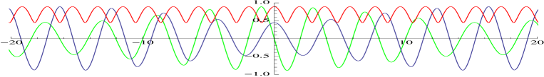
Figure 2: The graphic for the $\phi_{1}$ (green), $\phi_{2}$ (blue) and $\phi_{3}$ (red) as function of $x^{3}$ for a choice of the parameters $A_{1}=0.2,A_{2}=0.8,\psi_{1}=0.9,\mathcal{B}=1,\lambda=1,B_{1}=1,s_{1}=-1,s_{2}=-1$ . Accordingly, the wave vectors for the phase and pseudo-phase have been chosen to be $\alpha_{\mu}=\left(0,0,0,0.33541\right)$ and $\beta_{\mu}=\left(1.49638,1,0,-1.49638\right)$, respectively

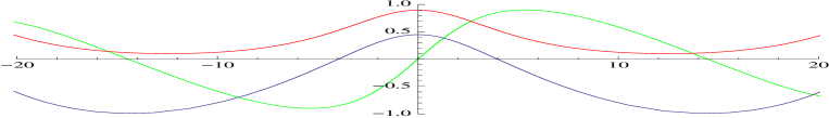
Figure 3: The graphic for the $\phi_{1}$ (green), $\phi_{2}$(blue) and $\phi_{3}$ (red) for a choice of the parameters $A_{1}=0.2,A_{2}=0.99,\psi_{1}=20.01,\mathcal{B}=1,\lambda=1,B_{1}=1,s_{1}=-1,s_{2}=-1$. The wave vectors are $\alpha_{\mu}=\left(0,0,0,-1.58153\right)$ and $\beta_{\mu}=\left(-1.04879,1,0,1.04879\right)$, respectively

Figure 4: Projection on the plane $\left(\phi_{1},\phi_{2}\right)$ of a sample of about 5000 consecutive values of the field $\phi$ along the axes $\left(0,0,x^{3}\right)$, for the same choice of parameters as in Figure 2

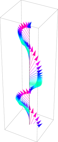
Figure 5: A sample of 200 consecutive spin configurations along the $x^{3}$ axis, with parameters as in Figure 2.

References

- [1] N. D. Mermin, T.-L. Ho: “Circulation and angular momentum in the A phase of superfluid 3He”, Phys. Rev. Lett. 36, 594 (1976).
- [2] L. M. Pismen: “Vortices in Nonlinear Fields”, Oxford University Press (1999).
- [3] G. E. Volovik: “The Universe in a Helium Droplet”, Oxford University Press (2003).
- [4] L. D. Faddeev, A. J. Niemi, Phys. Rev. Lett. 82, 1624 (1999); Phys. Lett. B 449, 214 (1999).
- [5] L. D. Faddeev, A. J. Niemi : “Spin-Charge Separation, Conformal Covariance and the SU(2) Yang–Mills Theory”, Nucl. Phys. B 776, 38 (2007).
- [6] G. I. Martone, “Separazione spin-carica nella teoria di Yang-Mills SU(2)”,master degree in Physics thesis, Lecce (2011).
- [7] V. I. Arnold, B. A. Khesin: “Topological Methods in Hydrodynamics”’, Springer-Verlag, New York (1998).
- [8] A. F. Vakulenko, L. V. Kapitanski: “Stability of solitons in S2 in the nonlinear -model”, Dokl. Akad. Nauk USSR 246, 840 (1979).
- [9] A. Kundu, Y. P. Rybakov: “Closed-vortex-type solitons with Hopf index”, J. Phys. A: Math. Gen. 15, 269 (1982).
- [10] J. Gladikowski and M. Hellmund: “Static solitons with nonzero Hopf number”, Phys. Rev. D 56, 5194 (1997).
- [11] L. Martina, G.I. Martone and S. Zykov: ”Symmetry reductions of the Skyrme – Faddeev model”, Acta Math. Appl. (2012), 1-12
- [12] L. D. Faddeev, A. J. Niemi, “Stable knot-like structures in classical field theory”, Nature 387, 58 (1997).
- [13] R. A. Battye, P. M. Sutcliffe: “Solitons, Links and Knots”, Proc. R. Soc. Lond. A 455, 4305 (1999).
- [14] J. Hietarinta, P. Salo: “Faddeev–Hopf knots: dynamics of linked un-knots”, Phys. Lett. B 451, 60 (1999).
- [15] J. Hietarinta, P. Salo: “Ground state in the Faddeev–Skyrme model”, Phys. Rev. D 62, 081701(R) (2000).
- [16] P. Sutcliffe: “Knots in the Skyrme–Faddeev model”, Proc. R. Soc. A 463, 3001 (2007).
- [17] R. S. Ward: “Hopf solitons on S3 and R3”, Nonlinearity 12, 241 (1999).
- [18] A. P. Protogenov: “Knots and Links of the Order Parameter Distributions in Strongly Correlated Systems”, Physics - Uspekhi 49 (7), 667 (2006).
- [19] J. Silva Lobo, R.S. Ward:” Generalized Skyrme Crystals”, Phys. Lett. B 696 (2011) 283-287
- [20] O. Alvarez, L. A. Ferreira and J. Sanchez-Guillen:”Integrable theories and loop spaces: fundamentals, applications and new developments”, Int.J.Mod.Phys. A24 (2009) 1825-1888
- [21] G.B. Whitham: ” Linear and Nonlinear Waves” , Wiley Intersci., New York - London - Sydney, 1974.
- [22] E. Infeld, G. Rowlands: ” Nonlinear waves, solitons and Chaos”, (Cambridge University Press, Cambridge, 1990).
- [23] S. Lee et al:” Single ferroelectric and chiral magnetic domain of single-crystalline BiFeO3 in an electric field”, Phys. Rev. B 78 (2008) 100101
- [24] E.V. Ferapontov, M.V. Pavlov, Hydrodynamic reductions of the heavenly equation, Class. Quantum Grav. 20 (2003) 2429-2441.
- [25] E.V. Ferapontov, K.R. Khusnutdinova, S.P. Tsarev, On a class of three-dimensional integrable Lagrangians. Comm. Math. Phys. 261 (2006), no. 1, 225 243