THE GALACTIC CENTER S-STARS AND THE HYPERVELOCITY STARS IN THE GALACTIC HALO: TWO FACES OF THE TIDAL BREAKUP OF STELLAR BINARIES BY THE CENTRAL MASSIVE BLACK HOLE?

Abstract

In this paper, we investigate the link between the hypervelocity stars (HVSs) discovered in the Galactic halo and the Galactic center (GC) S-stars, under the hypothesis that they are both the products of the tidal breakup of the same population of stellar binaries by the central massive black hole (MBH). By adopting several hypothetical models for binaries to be injected into the vicinity of the MBH and doing numerical simulations, we realize the tidal breakup processes of the binaries and their follow-up dynamical evolution. We find that many statistical properties of the detected HVSs and GC S-stars could be reproduced under some binary injecting models, and their number ratio can be reproduced if the stellar initial mass function is top-heavy (e.g., with slope $\sim-1.6$). The total number of the captured companions is $\sim 50$ that have masses in the range $\sim 3$–$7M_{\odot}$ and semimajor axes $\mathrel{\mathchoice{\lower 4.0pt\vbox{\halign{$\nms\displaystyle\hfil#\hfil$\cr<\crcr\sim\crcr}}}{\lower 4.0pt\vbox{\halign{$\nms\textstyle\hfil#\hfil$\cr<\crcr\sim\crcr}}}{\lower 4.0pt\vbox{\halign{$\nms\scriptstyle\hfil#\hfil$\cr<\crcr\sim\crcr}}}{\lower 4.0pt\vbox{\halign{$\nms\scriptscriptstyle\hfil#\hfil$\cr<\crcr\sim\crcr}}}}4000{\rm AU}$ and survive to the present within their main-sequence lifetime. The innermost one is expected to have a semimajor axis $\sim 300$–$1500{\rm AU}$ and a pericenter distance $\sim 10$–$200{\rm AU}$, with a significant probability of being closer to the MBH than S2. Future detection of such a closer star would offer an important test to general relativity. The majority of the surviving ejected companions of the GC S-stars are expected to be located at Galactocentric distances $\mathrel{\mathchoice{\lower 4.0pt\vbox{\halign{$\nms\displaystyle\hfil#\hfil$\cr<\crcr\sim\crcr}}}{\lower 4.0pt\vbox{\halign{$\nms\textstyle\hfil#\hfil$\cr<\crcr\sim\crcr}}}{\lower 4.0pt\vbox{\halign{$\nms\scriptstyle\hfil#\hfil$\cr<\crcr\sim\crcr}}}{\lower 4.0pt\vbox{\halign{$\nms\scriptscriptstyle\hfil#\hfil$\cr<\crcr\sim\crcr}}}}20\rm~{}kpc$, and have heliocentric radial velocities $\sim-500$–$1500{\rm km\,s^{-1}}$ and proper motions up to $\sim 5$–$20{\rm mas\,yr^{-1}}$. Future detection of these HVSs may provide evidence for the tidal breakup formation mechanism of the GC S-stars.

1. Introduction

More than a hundred young massive stars, mostly Wolf Rayet/O and B types, have been identified within a distance of $\sim 0.5{\rm~{}pc}$ from the massive black hole (MBH) in the Galactic center (GC; Gillessen et al., 2009; Lu et al., 2009; Bartko et al., 2010). These young stars are empirically divided into two groups: (1) the majority of the young stars at a distance $\sim 0.04$–$0.5{\rm~{}pc}$ from the MBH are located on coherent disk-like structures, i.e., the clockwise rotating stellar (CWS) disk and the possible counterclockwise rotating stellar (CCWS) disk (e.g., Levin & Beloborodov, 2003; Paumard et al., 2006; Lu et al., 2009); and (2) the young stars within a distance of $0.04{\rm~{}pc}$ from the MBH (denoted as GC S-stars), exclusively B-dwarfs, are spatially isotropically distributed and their orbital eccentricities follow a distribution of $f_{e}(e)\propto e^{2.6}$ (e.g., Ghez et al., 2008; Gillessen et al., 2009). The existence of these young stars is quite puzzling as star formation in the vicinity of an MBH is thought to be strongly suppressed due to the tidal force from the MBH (i.e., the paradox of youth; see Ghez et al., 2008; Paumard et al., 2006). It is of great importance to address not only the formation of these stars but also the origin of their kinematics, which should encode fruitful information of the dynamical interplays between the central MBH and its environment.

Young stars in the CWS (or CCWS) disk are probably formed in a previously existing massive gaseous disk due to instabilities and fragmentation developed in it (e.g., Levin, 2007; Nayakshin, 2006; Alexander et al., 2008; Bonnell & Rice, 2008). Young binary stars in the disk(s) may migrate or be scattered into the vicinity of the central MBH (e.g., Madigan et al., 2009) and then be tidally broken up (e.g., Hills, 1988; Yu & Tremaine, 2003). One component of a broken-up binary may be ejected out as a hypervelocity star (HVS) as discovered in the Galactic halo (e.g., Brown et al., 2005; Edelmann et al., 2005; Hirsch et al., 2005), and the other component may be captured onto a tighter orbit similar to that of the GC S-stars as proposed by Gould & Quillen (2003). If HVSs were initially originated from a stellar structure like the CWS disk, they may be spatially located close to the disk plane (Lu et al., 2010). The current observations do show such a spatial correlation between the HVSs and the CWS disk, which suggests that majority of the HVSs originate from the CWS disk (Lu et al., 2010; Zhang et al., 2010).

The HVSs discovered in the Galactic halo and the GC S-stars in the vicinity of the central MBH may naturally link to each other as they may both be the products of the tidal breakup of stellar binaries in the vicinity of the central MBH (e.g., Ginsburg & Loeb, 2006). Therefore, it is interesting to simultaneously investigate the properties of the HVSs in the Galactic halo (or the GC S-stars) and their captured (or ejected) companions, and probability distribution of these properties. Under the assumption that both the HVSs and GC S-stars are the products of tidal breakup of stellar binaries, the working hypothesis in this paper, we construct a number of Monte Carlo models to simulate the tidal breakup processes of stellar binaries in the GC and check whether these models can accommodate the current observations, and make further predictions on both the companions of HVSs and that of GC S-stars for future observations.

This paper is organized as follows. In Section 2, we overview the tidal breakup processes of stellar binaries in the vicinity of an MBH and the dynamical connection between the ejected and captured components. Adopting relatively realistic initial conditions, we perform a large number of three-body experiments to realize the tidal breakup processes of stellar binaries in Section 3. Assuming a constant injection rate of stellar binaries into the vicinity of the central MBH and adopting the results from the three-body experiments on the ejected and captured components, we use the Monte Carlo simulations to produce both the HVSs and the GC S-stars. In Section 4, we follow the orbital evolution of the captured stars to the present time by adopting the autoregressive moving average (ARMA) model (Madigan et al., 2011), in which both the non-resonant relaxation (NR) and the resonant relaxation (RR) are included. The simulated GC S-stars appear to be compatible with the observations of the GC S-stars. In Section 5, we investigate the effects of different binary injection models on the number ratio of the simulated HVSs to GC S-stars. The number ratio given by observations can be reproduced if the initial mass function (IMF) of the primary components of stellar binaries is somewhat top-heavy. By calibrating the injection models with observations, we estimate the number of the captured (or ejected unbound) stars, as the companions of HVSs (or GC S-stars), that could be detected in the future. We also estimate the probability to have less massive stars captured on an orbit within that of S2 in Section 6. Conclusions are given in Section 7.

For clarity, some notations of the variables that are frequently used in this paper are summarized in Table 1. Given a physical variable $X$ (e.g., mass, velocity, semimajor axis, eccentricity), the distribution function of $X$ is denoted by $f_{X}(X)$ so that $f_{X}(X)dX$ represents the number of relevant objects with variable $X$ being in the range $X\rightarrow X+dX$.

Table 1Notation of Some Symbols

Symbol	Description
$M_{\bullet}$	Mass of the central MBH
$m_{\rm p}$	Mass of the primary component of an injecting stellar binary
$m_{\rm s}$	Mass of the secondary component of an injecting stellar binary
$m$	Total mass of an injecting stellar binary, i.e., $m_{\rm p}+m_{\rm s}$
$R$	$m_{\rm s}/m_{\rm p}$
$a_{\rm b,ini}$	Initial semimajor axis of an injecting stellar binary
$r_{\rm p,ini}$	Initial pericenter distance of the mass center of the injecting stellar binary to the MBH
$a_{\rm b-\bullet,ini}$	Initial semimajor axis of the orbit of an injecting stellar binary rotating around a central MBH
$v_{\rm\infty,ini}$	Initial velocity of the injecting stellar binary at infinity if the binary is on a hyperbolic orbit
$E_{\rm ini}$	Initial energy of the stellar binary
$r_{\rm tb}$	Tidal radius for the stellar binary
$D$	Orbital penetration parameter of the injecting stellar binary ($\equiv 100r_{\rm p,ini}/r_{\rm tb}$)
$\alpha$	Exponent of the power-law distribution of $a_{\rm b,ini}$
$\beta$	Exponent of the power-law distribution of $r_{\rm p,ini}$
$\gamma$	Exponent of the power-law distribution of $m_{\rm p}$
$m_{\rm g}$	Mass of the component that gains energy during the tidal breakup of a stellar binary
$m_{\rm l}$	Mass of the component that loses energy during the tidal breakup of a stellar binary
$q$	$m_{\rm l}/m_{\rm g}$
$\delta E$	Exchange energy between the two components during the tidal breakup of a stellar binary
$m_{\rm ej}$	Mass of the ejected star after the tidal breakup of a stellar binary
$m_{{\rm cap}}$	Mass of the captured star after the tidal breakup of a stellar binary
$v_{\infty}$	Velocity of the ejected component at infinity
$a_{{\rm cap}}$	Orbital semimajor axis of the captured component
$a_{\rm cap,0}$	Orbital semimajor axis of the captured component if the injecting binary is initially on a parabolic orbit
$e_{{\rm cap}}$	Orbital eccentricity of the captured component
$N_{{\rm HVS}}^{{\rm tot}}$	Simulated total number of the ejected stars given a mass range
$N_{{\rm cap}}^{{\rm tot}}$	Simulated total number of the captured stars given a mass range
$N_{{\rm HVS}}^{\rm obs}$	Simulated number of the detectable HVSs at the present time for given selection criteria
$N_{{\rm cap}}^{\rm obs}$	Simulated number of the detectable captured stars at the present time for given selection criteria
$F_{{\rm HVS}}^{{\rm lt}}$	Simulated fraction of the ejected stars that survive to the present time on the main sequence
$F_{{\rm cap}}^{{\rm lt}}$	Simulated fraction of the captured stars that survive to the present time on the main sequence
$F_{{\rm cap}}^{{\rm td}}$	Simulated fraction of the captured stars that have already been tidally disrupted until the present time
$F_{{\rm cap}}^{\rm obs}$	Simulated fraction of the captured stars that can be detected at the present time for given selection criteria

2. Overview: tidal breakup of stellar binaries in the vicinity of an MBH

A stellar binary may be broken up if it approaches an MBH within a distance of $r_{\rm tb}=a_{\rm b}(3M_{\bullet}/m)^{1/3}$, where $M_{\bullet}$ is the mass of the MBH, $a_{\rm b}$ is the semimajor axis of the binary, $m=m_{\rm g}+m_{\rm l}$ is the total mass of the binary, and $m_{\rm g}$ and $m_{\rm l}$ are the masses of the two components of the binary, respectively. During the breakup, one component of the binary, denoted as $m_{\rm g}$ here, gains energy, and the other component $m_{\rm l}$ loses energy. For an injecting stellar binary that is initially on a parabolic orbit relative to the MBH, the velocity of the binary mass center at its periapsis to the MBH ($\sim r_{\rm tb}$) is $v_{\rm tb}\sim(GM_{\bullet}/r_{\rm tb})^{1/2}$. The component $m_{\rm g}$ receives a velocity change on the order of $\delta v_{\rm g}\sim(m_{\rm l}/m)\sqrt{Gm/a_{\rm b}}$ if the eccentricity of the stellar binary is $0$, and it gains energy $\delta E\sim m_{\rm g}v_{\rm tb}\delta v_{\rm g}$. The other component $m_{\rm l}$ loses the same amount of energy $\delta E$. If $\delta E$ is sufficiently large, the component $m_{\rm g}$ may manifest itself as an HVS with velocity at infinity $v_{\infty}\sim\sqrt{2\delta E/m_{\rm g}}$ if ignoring the deceleration due to the Galactic gravitational potential. The root mean square (rms) of $v_{\infty}$ is approximately

$$\left<v^{2}_{\infty}\right>^{1/2} \sim v_{\infty,0}\left(\frac{0.1{\rm AU}}{a_{\rm b}}\right)^{1/2}\left(\frac{m}{6M_{\odot}}\right)^{1/3}$$ (1)

$$\times \left(\frac{2m_{\rm l}}{m}\right)^{1/2}\left(\frac{M_{\bullet}}{4\times 10^{6}M_{\odot}}\right)^{1/6}g(D),$$

where $v_{\infty,0}=2596{\rm km\,s^{-1}}$ and $g(D)$ is given by Bromley et al. (2006) for injecting binaries on hyperbolic orbits with initial velocities at infinity of $250{\rm km\,s^{-1}}$, i.e.,

$$g(D) = 0.774+0.0245D-8.99\times 10^{-4}D^{2}$$ (2)

$$+1.32\times 10^{-5}D^{3}-8.82\times 10^{-8}D^{4}$$

$$+2.15\times 10^{-10}D^{5},$$

where the penetration parameter $D\equiv 100r_{\rm p,ini}/r_{\rm tb}$ characterizes the minimum distance where the binary approaches the MBH, and $r_{\rm p,ini}$ is the initial pericenter distance of the binary. The rms velocity $\left<v^{2}_{\infty}\right>^{1/2}$ apparently depends on the semimajor axis, the total mass and the mass ratio of the stellar binary, and the penetration parameter $D$.

The exact value of $v_{\infty}$ of the ejected component for any given stellar binary also depends on the relative orientation of the stellar binary orbital plane to the orbital plane of the binary rotating around the MBH and the orbital phases of the two components at the time of its breakup. This dependence introduces a scatter of $v_{\infty}$ around the value $\left<v^{2}_{\infty}\right>^{1/2}$ given by Equation (1), as the orbital orientations of the injecting stellar binaries are probably random and the orbital phases of the two components are not fixed at the breakup time. Numerical simulations have shown that this scatter is approximately Gaussian with a dispersion of $\sigma_{v_{\infty}}\sim 0.2\left<v^{2}_{\infty}\right>^{1/2}$ (Bromley et al., 2006; Zhang et al., 2010), where the binary orbital orientations are assumed to be randomly distributed. The symmetry of the orbital phases of the two binary components (always at the opposite side to the mass center of the binary) ensures the same probability of receiving energy for each star, which leads to the same ejection probability for both components if the injecting binaries are initially on parabolic orbits (Sari et al., 2010; Kobayashi et al., 2012).

Stellar binaries on orbits bound to the MBH may experience multiple close encounters with the MBH and the binary semimajor axes and eccentricities may be cumulatively excited to larger values until finally being broken up (Zhang et al., 2010). The distribution of $v_{\infty}$ for the ejected stars, produced during the first encounters of the binaries with the MBH, follows a fitting formula similar to Equation (2) over $D\sim 20$–$150$, i.e., $g(D)\propto 1-(D/256)^{2}$, as the initial bounding energy of the injecting stellar binaries is still significant (for details, see Zhang et al., 2010). For multiple encounters, the energy exchange $\delta E$ between the two components is determined by the properties of the stellar binaries at the final revolutions. Our simulations show that $\left<v^{2}_{\infty}\right>^{1/2}$ of those ejected components for stellar binaries broken up within $1000$ revolutions around the MBH still follows Equation (1), but $g(D)$ is now best fitted by

$$g(D) = 0.912-2.41\times 10^{-4}D-4.49\times 10^{-5}D^{2}$$ (3)

$$+2.68\times 10^{-7}D^{3}-4.42\times 10^{-10}D^{4},$$

for $D<300$.

For stellar binaries on bound orbits, the light component has a larger probability to escape away from the MBH because the specific energy it could gain is generally larger than that of the heavy component in a counterpart case (see Equation 1). However, the difference in the ejection probability for the two components of the stellar binaries is significant only when the mass ratio of the massive ones to the light ones $\mathrel{\mathchoice{\lower 4.0pt\vbox{\halign{$\nms\displaystyle\hfil#\hfil$\cr>\crcr\sim\crcr}}}{\lower 4.0pt\vbox{\halign{$\nms\textstyle\hfil#\hfil$\cr>\crcr\sim\crcr}}}{\lower 4.0pt\vbox{\halign{$\nms\scriptstyle\hfil#\hfil$\cr>\crcr\sim\crcr}}}{\lower 4.0pt\vbox{\halign{$\nms\scriptscriptstyle\hfil#\hfil$\cr>\crcr\sim\crcr}}}}5$ and $2\delta E/m_{\rm g}$ is close to its initial bounding energy $GM_{\bullet}/2a_{\rm b-\bullet,{\rm ini}}$, where $a_{\rm b-\bullet,{\rm ini}}$ denotes the initial semimajor axis of the binary system composed of a stellar binary and the MBH (see also Antonini et al., 2011; Kobayashi et al., 2012).

The component $m_{\rm l}$ of a broken-up stellar binary loses energy by an amount of $\delta E$ and it is captured onto a tighter orbit with semimajor axis $a_{\rm cap}$. According to the energy conservation law, we roughly have

$$\frac{1}{2}m_{\rm g}v_{\infty}^{2}-\frac{Gm_{\rm l}M_{\bullet}}{2a_{\rm cap}}\simeq E_{{\rm ini}},$$ (4)

where $E_{{\rm ini}}$ is the initial energy of the stellar binary, and it is $\sim\frac{1}{2}mv_{\infty,{\rm ini}}^{2}$ if the binary is initially on a hyperbolic orbit, or $\sim-GmM_{\bullet}/(2a_{\rm b-\bullet,{\rm ini}})$ if on a bound orbit. The initial internal mechanical energy of the stellar binary $-\frac{Gm_{l}m_{g}}{2a_{\rm b,ini}}$ is ignored in Equation (4). We now have the general form for $v_{\infty}$ as $v_{\infty}\sim\sqrt{2(\delta E+\frac{m_{\rm g}}{m}E_{{\rm ini}})/m_{\rm g}}$. If $|E_{{\rm ini}}|\ll\delta E$, the semimajor axis of the captured star is

$$a_{\rm cap} \simeq a_{\rm cap,0}=q\frac{GM_{\bullet}}{v^{2}_{\infty}}$$ (5)

$$= 3500q{\rm AU}\left(\frac{M_{\bullet}}{4\times 10^{6}M_{\odot}}\right)\left(\frac{1000{\rm km\,s^{-1}}}{v_{\infty}}\right)^{2},$$

where $q\equiv m_{\rm l}/m_{\rm g}$. For the cases considered in this paper, the injecting stellar binaries are either initially on hyperbolic orbits (but close to parabolic ones) or from stellar structures like the CWS disk, and thus $a_{\rm cap}\sim a_{\rm cap,0}$ as approximately $|E_{{\rm ini}}|\ll\delta E$. Equation (5) shows the connection between the properties of the captured stars left in the GC and that of their ejected companions in the Galactic bulge and halo. For those HVSs discovered in the Galactic halo with $v_{\infty}\sim 700$-$1000{\rm km\,s^{-1}}$, their companions left in the GC may be initially on orbits with semimajor axis in the range of $\sim 3500$-$7000{\rm AU}$ as stellar binaries with extreme mass ratios are rare. For the innermost S-star, i.e., the S2, of which the semimajor axis is $\sim 1000{\rm AU}$, its companion ejected out should have $v_{\infty}\sim 1900{\rm km\,s^{-1}}$ if $q\sim 1$, and $\sim 600{\rm km\,s^{-1}}$ if $q\sim 0.1$, respectively. For stellar binaries initially tightly bound to the MBH, we may have $\delta E+\frac{m_{\rm g}}{m}E_{{\rm ini}}\mathrel{\mathchoice{\lower 4.0pt\vbox{\halign{$\nms\displaystyle\hfil#\hfil$\cr<\crcr\sim\crcr}}}{\lower 4.0pt\vbox{\halign{$\nms\textstyle\hfil#\hfil$\cr<\crcr\sim\crcr}}}{\lower 4.0pt\vbox{\halign{$\nms\scriptstyle\hfil#\hfil$\cr<\crcr\sim\crcr}}}{\lower 4.0pt\vbox{\halign{$\nms\scriptscriptstyle\hfil#\hfil$\cr<\crcr\sim\crcr}}}}0$, the component gaining energy either remains bound to the MBH or is ejected out with low velocities.

The distribution of HVS properties is directly connected to the distribution of S-star properties (note that here we do not mean that an observed HVS in the Galactic halo is directly associated with an observed GC S-star as the products of the tidal breakup of the same binary star). According to Equation (5), the distribution of the semimajor axis of the captured stars $f_{a_{\rm cap}}$ is related to the distribution of the velocity of HVSs at infinity $f_{v_{\infty}}$ if $m_{\rm g}\sim m_{\rm l}$, i.e.,

$$f_{v_{\infty}}(v_{\infty})\propto\left.a_{\rm cap}^{3/2}f_{a_{\rm cap}}(a_{\rm cap})\right|_{a_{\rm cap}=\frac{GM_{\bullet}}{v_{\infty}^{2}}},$$ (6)

which suggests that any one of the two distributions above can be inferred from the other one.

The velocity distribution of the ejected stars are mainly determined by the initial sets on the distributions of $a_{\rm b,ini}$ and $r_{\rm p,ini}$ since

$$\left<v^{2}_{\infty}\right>^{1/2}\propto a_{\rm b,ini}^{-1/2}g(D),$$ (7)

where $g(D)$ denotes the dependence of the rms velocity $\left<v^{2}_{\infty}\right>^{1/2}$ on the penetration parameter $D$, as shown in Equations (2) and (3) for the cases of injecting binaries initially on hyperbolic orbits but close to parabolic ones and bound orbits like the stars in the CWS disk, respectively. The fitting forms of $g(D)$ obtained from numerical experiments (Equations (2) and (3)) are decreasing functions in the range of $20<D<150$ or $20<D<300$, and thus $g(D)$ may be approximated as a monotonically decreasing function. We assume that the initial distribution of $a_{\rm b,ini}$ and $r_{\rm p,ini}$ are $f_{a_{\rm b}}(a_{\rm b,ini})\propto a_{\rm b,ini}^{\alpha}$ and $f_{r_{\rm p}}(r_{\rm p,ini})\propto r_{\rm p,ini}^{\beta}$, respectively; and the probability of a stellar binary with semimajor axis $a_{\rm b,ini}$ broken up by the central MBH at a penetration distance $D$ is only a function of $D$, i.e., $f_{D}(D)$ (see Bromley et al., 2006). If $q\sim 1$ and ignoring the scatter of $v_{\infty}$ around $\left<v_{\infty}^{2}\right>^{1/2}$ (i.e., $v_{\infty}\sim\left<v^{2}_{\infty}\right>^{1/2}$), the velocity distribution of the ejected components can be obtained as

$$f_{v_{\infty}}(v_{\infty}) \propto \frac{\partial}{\partial v_{\infty}}\int\int f_{a_{\rm b}}(a_{\rm b,ini})f_{r_{\rm p}}(r_{\rm p,ini})\times$$ (8)

$$f_{D}(D)da_{\rm b,ini}dr_{\rm p,ini}$$

$$\propto \frac{\partial}{\partial v_{\infty}}\int a_{\rm b,ini}^{\alpha+\beta+1}da_{\rm b,ini}\int D^{\beta}f_{D}(D)dD$$

$$\propto v_{\infty}^{-2\alpha-2\beta-5},$$

and this relation is valid only if $g(D)$ is a monotonically decreasing function and it is independent of the detailed form of $f_{D}(D)$. Similarly, we also have

$$f_{a_{\rm cap}}(a_{\rm cap})\propto a_{\rm cap}^{\alpha+\beta+1},$$ (9)

which is consistent with the simple relation given by Equation (6). The estimated slope of $f_{v_{\infty}}(v_{\infty})$ (or $f_{a_{\rm cap}}(a_{\rm cap})$) above is not affected by taking account of the Gaussian-like scatter of $v_{\infty}$ around $\left<v^{2}_{\infty}\right>^{1/2}$ as the distribution is a power law. If considering of the various mass ratios among the injecting binaries (see Equations (1) and (5)), however, the resulted slope of $f_{v_{\infty}}(v_{\infty})$ may be somewhat flatter than the simple estimates above. Note also that a larger $\beta$ may correspond to a slower migration/diffusion of stellar binaries into the low angular momentum orbits or the vicinity of the central MBH, and lead to fewer HVSs at the high-velocity end and fewer captured stars in smaller distances to the MBH.

The periapsis of a captured star $m_{\rm l}$ is roughly $\sim r_{\rm tb}$ and the characteristic eccentricity of the captured star is

$$\bar{e}_{{\rm cap}}\sim 1-\frac{r_{\rm tb}}{a_{\rm cap}}\simeq 1-\frac{2.8}{q^{1/3}(1+q)^{2/3}}\left(\frac{m_{\rm l}}{M_{\bullet}}\right)^{1/3}.$$ (10)

the $\bar{e}_{{\rm cap}}$ depends on $q$ and the mass ratio of the captured star to the MBH. Considering of the Gaussian-like scatter in $v_{\infty}$ and correspondingly the scatter in $a_{\rm cap}$, the probability that the breakup of a stellar binary with given semimajor axis and mass of each component results in a captured star with eccentricity $<e_{\rm cap}$ is roughly

$$P(<e_{\rm cap})=\frac{1}{2}{\rm erfc}\left[\frac{\sqrt{(1-e_{\rm cap})/(1-\bar{e}_{{\rm cap}})}-1}{\sqrt{2}\sigma_{v_{\infty}}/\langle v^{2}_{\infty}\rangle^{1/2}}\right],$$ (11)

where $\bar{e}_{{\rm cap}}$ is given by Equation (10) and $\sigma_{v_{\infty}}/\langle v^{2}_{\infty}\rangle^{1/2}\simeq 0.2$. To capture an S2-like star (i.e., $e_{\rm cap}\simeq 0.887$ and $m_{\rm l}\sim 15M_{\odot}$; see Ghez et al. 2008; Gillessen et al. 2009) directly through the tidal breakup of stellar binaries, it is necessary to have $m_{\rm g}\gg m_{\rm l}\sim 15M_{\odot}$ ($q\ll 1$) and the probability is $\sim 0.25$ if $q=0.1$ according to Equation (11) (see Gould & Quillen, 2003). The probability to capture stars onto orbits with $e_{\rm cap}<0.8$ is only $\sim 10^{-17}$ if $m_{\rm g}=m_{\rm l}=15M_{\odot}$; and $\sim 6\times 10^{-3}$ even if $m_{\rm g}=10m_{\rm l}=150M_{\odot}$ (see also Gould & Quillen 2003). Since the number of GC S-stars is only on the order of a few tens, it is difficult to produce all the nine observed GC S-stars with eccentricities $<0.8$ (Gillessen et al., 2009) directly by the tidal breakup of stellar binaries. In addition, the captured stars may initially remain on a disk plane if their progenitor binaries are originated from disk-like stellar structure(s) as suggested by Lu et al. (2010), which is different from the isotropic distribution of the GC S-stars. Therefore, additional physical mechanism is required to further make the captured stars evolve to orbits with lower eccentricities and spatially isotropically distributed if the GC S-stars are really originated from the tidal breakup of binary stars.

The processes, initially proposed by Rauch & Tremaine (1996), may cause the captured stars dynamically evolving to their present orbits as discussed by a number of authors (Levin, 2007; Hopman & Alexander, 2006; Kocsis & Tremaine, 2011). In Section 4, we will take into account the relaxation processes, including RR, to approximately follow the dynamical evolution of each “GC S-star” after its capture due to the tidal breakup of stellar binaries; we then check whether the eccentricity and spatial distributions of those surviving “GC S-stars” are compatible with current observations. Note here we use the quotes around the term GC S-stars to represent all of those captured stars with mass in the range of $\sim 7$-$15M_{\odot}$; while the simulated GC S-stars (without quotes) represent those with mass $\sim 7$-$15M_{\odot}$ surviving to the present time, which presumably correspond to the observed ones (see Section 4).

3. Monte Carlo Simulations

In this section, we first adopt Monte Carlo simulations to realize the tidal breakup processes and generate HVSs and “GC S-stars”, and then we investigate in detail the connection between the simulated HVSs and “GC S-stars”. We use the code DORPI5 based on the explicit fifth (fourth)-order Runge–Kutta method (Dormand & Prince, 1980; Hairer et al., 1993) to calculate the three-body interactions between a stellar binary and the central MBH. For details of the numerical calculations, see Zhang et al. (2010). The successive dynamical evolution of the captured stars in the GC and the kinematic motion of the produced HVSs in the Galactic potential will be discussed in Sections 4 and 5, respectively.

3.1. Initial Settings

The mass of the central MBH is set to be $4\times 10^{6}M_{\odot}$ throughout the numerical calculations in this paper (Ghez et al., 2008; Gillessen et al., 2009).

For the injecting stellar binaries, the initial conditions are set as follows:

• The distribution of the semimajor axes $a_{\rm b,{\rm ini}}$ follows the Öpik law, i.e., $\alpha=-1$ (e.g., Kobulnicky & Fryer, 2007).

• The mass distribution of the primary stars $m_{\rm p}$ follows a power law function, $f_{m_{\rm p}}(m_{\rm p})\propto m_{\rm p}^{\gamma}$. The distribution of the secondary star ($m_{\rm s}$) or the mass ratio $R\equiv m_{\rm s}/m_{\rm p}$ can be described by two populations: (1) a twin population, i.e., about 40% of binary stars have $R\sim 1$, and (2) the rest binaries, which follow a distribution of $f_{R}(R)\sim{\rm constant}$ (Kobulnicky & Fryer, 2007; Kiminki et al., 2008, 2009).

• The initial eccentricity of the injecting binary is assumed to be $e_{{\rm ini}}=0$, as adopted in previous works (e.g., Bromley et al. 2006; Antonini et al. 2010).

• The orientation of the inner binary orbital plane is chosen to be uniformly distributed in $\cos\phi$ for $\phi\in(0,\pi)$.

For the orbits of the injecting stellar binaries relative to the central MBH, the initial conditions are set as follows:

• The stellar binaries are assumed to be initially injected from either disk-like stellar structures (similar to the CWS disk) or infinity. If they were from structures like the CWS disk, the semimajor axes $a_{\rm b-\bullet,{\rm ini}}$ follows a power-law distribution proportional to $a_{\rm b-\bullet,ini}^{-2.3}$ in the range of $\sim 0.04$-$0.5{\rm~{}pc}$ according to current observations on the CWS disk (Lu et al., 2009; Bartko et al., 2009). If they were from infinity, i.e., unbound to the MBH, their initial velocities at infinity are set to $v_{\rm\infty,ini}=250{\rm km\,s^{-1}}$.

• If the injecting binaries were from disk-like stellar structures, the orientations of their orbits relative to the MBH are assumed to satisfy a Gaussian distribution around the central planes of the stellar disks with a standard deviation of $12{{}^{\circ}}$ (cf. Lu et al., 2009; Bartko et al., 2009). The planes of the host disks are assumed to be the same as the two planes that best fit the observations, i.e., $(l,b)=(311{{}^{\circ}},-14{{}^{\circ}})$ and $(176{{}^{\circ}},-53{{}^{\circ}})$, respectively, and these two planes are consistent with the CWS disk plane and the plane of the northern arm (Narm) of the mini-spiral in the GC (or the outer warped part of the CWS disk; Lu et al. 2010; Zhang et al. 2010). The injection rates from these two disks are assumed to be the same.

• The periapsis that the injecting stellar binaries approach the MBH is simply assumed to follow a power law distribution, $f_{r_{\rm p}}(r_{\rm p,ini})\propto r_{\rm p,ini}^{\beta}$ and $\beta>0$. A larger value of $\beta$ corresponds to a smaller fraction of the injecting stellar binaries that could approach the immediate vicinity of the central MBH. It is still not clear which mechanism is responsible for the migration (or diffusion) of stellar binaries into the vicinity of the central MBH, although the secular instability developed in a stellar disk is proposed to be a viable one (Madigan et al., 2009). Instead of incorporating the detailed migration/diffusion process of the stellar binaries in the Monte Carlo simulations below, we choose to parameterize the migration/diffusion process qualitatively by different values of $\beta$ and a larger $\beta$ corresponds to a slower migration/diffusion process.

Table 2Different Injection Models for Tidal Breakup of Binaries

Model	$\gamma$	$\beta$	$a_{\rm b-\bullet,ini}({\rm~{}pc})$	$v_{\rm\infty,ini}({\rm km\,s^{-1}})$
Unbd-MS0	-2.7	0	$\cdots$	250
Disk-MS0	-2.7	0	0.04-0.5	$\cdots$
Disk-TH0	-0.45	0	0.04-0.5	$\cdots$
Disk-TH2	-0.45	2	0.04-0.5	$\cdots$

In this section, we perform Monte Carlo simulations by adopting four sets of initial conditions (as listed in Table 2). In the first model, the stellar binaries are assumed to be injected from infinity with initial velocity of $v_{\rm\infty,ini}=250{\rm km\,s^{-1}}$. For the primary components of the injecting binaries, we adopt the Miller Scalo IMF (e.g., Kroupa 2002). This model is denoted as “Unbd-MS0”. For the other three models, the stellar binaries are assumed to be originated from stellar structures like the CWS disk, and the IMF of the primary components is either set to be the Miller Scalo IMF or a top-heavy IMF with a slope of $\gamma=-0.45$ as suggested by recent observations of the disk stars (see Bartko et al., 2010). The slope of the initial distribution of the pericenter distance $\beta$ is set to be either $0$ or $2$. These models are denoted as “Disk-MS0”, “Disk-TH0”, and “Disk-TH2”, respectively. The total number of three-body experiments is $10^{5}$ for each model with the initial settings described above. By comparing the results obtained from those different models, one may be able to distinguish the effects of different settings on the IMF and the injection of stellar binaries.

If not specified, those ejected or captured stars with mass in the range of $\sim 3$-$15M_{\odot}$ are recorded, thus both the HVSs with mass $\sim 3$-$4M_{\odot}$ and the captured stars with mass $\sim 7$-$15M_{\odot}$, corresponding to the currently detected ones, can be taken into account simultaneously. The ejected or captured stars with mass in the range of $\sim 4$-$7M_{\odot}$ are also considered for completeness. For other ejected or captured stars with mass out of the range of $3$-$15M_{\odot}$, they may be either too faint to be detected or too massive with too short lifetime and thus with too small probability to survive.

3.2. Numerical Results

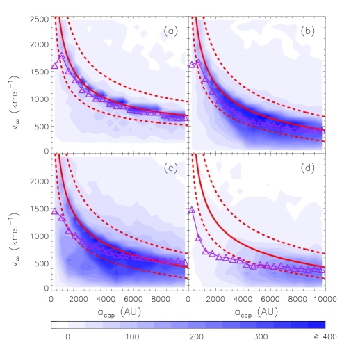
Figure 1.— Number distributions of broken-up stellar binaries in the $v_{\infty}$-$a_{\rm cap}$ plane, where $v_{\infty}$ is the velocity at infinity of the ejected component and $a_{\rm cap}$ is the semimajor axes of its captured companion. Panels (a)–(d) show results obtained from the Unbd-MS0, Disk-MS0, Disk-TH0, and Disk-TH2 models, respectively. The total number of the three-body experiments is $10^{5}$ for each model. The solid red line in each panel shows the estimation according to Equation (4) for $m_{\rm g}=m_{\rm l}$ by assuming $v_{\rm\infty,ini}=250{\rm km\,s^{-1}}$ in panel (a), and $a_{\rm b-\bullet,{\rm ini}}=0.2{\rm~{}pc}$ in panels (b)–(d), respectively. The dashed red lines above or below the solid lines represent the estimations for $m_{\rm g}/m_{\rm l}=1/2$ and $2$, respectively. The magenta lines with triangles indicate the rms of $v_{\infty}$ for each bin of $a_{\rm cap}$. The number of stars is counted in each of the $a_{\rm cap}$ and $v_{\infty}$ bins (totally $25\times 25$ bins with bin size $400{\rm AU}\times 100{\rm km\,s^{-1}}$) and represented by the color brightness scales shown in the label.

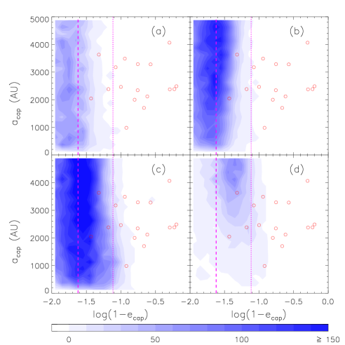
Figure 2.— Number distributions of the captured stars in the $a_{\rm cap}$ vs. $\log(1-e_{\rm cap})$ plane, where $a_{\rm cap}$ and $e_{\rm cap}$ are the semimajor axes and eccentricities of the captured stars achieved right after their capture, respectively. Panels (a)–(d) show the results from the Unbd-MS0, Disk-MS0, Disk-TH0, and Disk-TH2 model, respectively. The red open circles represent the observed GC S-stars with $a_{\rm cap}$ smaller than $4000{\rm AU}$ at the present time (Gillessen et al., 2009); and the magenta dashed and dotted lines are for the mean eccentricities given by Equation (10) for $(m_{\rm l},q)=(10M_{\odot},1)$ and $(10M_{\odot},1/10)$, respectively. The number of stars is counted in each of the $a_{\rm cap}$ and $\log(1-e_{\rm cap})$ bins (totally $25\times 25$ bins with bin size $200{\rm AU}\times 0.08$) and represented by the color brightness scales shown in the label.

Figure 1 shows the distribution of the tidally broken-up stellar binaries in the $v_{\infty}$-$a_{\rm cap}$ plane, where $v_{\infty}$ is the velocity at infinity of the ejected component and $a_{\rm cap}$ is the semimajor axis of the captured component. As shown in panel (a), the majority of the simulated $v_{\infty}$-$a_{\rm cap}$ pairs obtained from the Unbd-MS0 model are close to the one estimated from Equation (5) by setting $m_{\rm l}/m_{\rm g}=1$ (solid line). The main reasons for this are: (1) the majority ($70\%$) of the injecting stellar binaries have mass ratios $q=m_{\rm l}/m_{\rm g}$ in the range of (1/2, 2) under the assumption of two populations set for the stellar binaries; and (2) all the injecting binaries have the same but negligible initial energy $E_{{\rm ini}}$. A small number of $v_{\infty}$-$a_{\rm cap}$ pairs, which apparently deviate significantly away from the solid line (for $q=1$ obtained from Equation 5), are due to the breakup of the binaries with $q$ substantially larger or smaller than $1$ (below or above the solid line). For the other three models, the simulation results do not deviate far away from the simple predictions by Equation (4) (for $q=1$), except that fewer ejected stars at the high-velocity end are produced in the Disk-TH2 model than in the other models simply because not many stellar binaries can closely approach the MBH. The scatters of $v_{\infty}$ around that predicted by Equation (4) in panels (b)-(d) are more significant compared with that in panel (a), which is caused by one or the combination of the effects as follows: (1) a distribution of the negative initial energy of the injecting stellar binaries originated from stellar structure like the CWS disk (panels (b)-(d)); (2) relatively more progenitor binaries have $q$ substantially larger or smaller than $1$ in the cases with a top-heavy IMF (panels (c) and (d)); and (3) fewer stellar binaries approach the immediate vicinity of the central MBH in the case of a large $\beta$ (panel (d)).

As seen from Figure 1, if the observed GC S-stars, with semimajor axes $\sim 1000$-$4000{\rm AU}$, are produced by the tidal breakup of stellar binaries, their ejected companions are expected to have $v_{\infty}\sim 1000$-$1600{\rm km\,s^{-1}}$ in the Unbd-MS0 model and $\sim 200$-$1500{\rm km\,s^{-1}}$ in the other models. The Disk-TH2 model produces fewer ejected stars with $v_{\infty}$ substantially larger than $1000{\rm km\,s^{-1}}$ compared with other models. The captured companions of the detected HVSs in the Galactic halo are more likely to have $a_{\rm cap}\sim 3000$-$8000{\rm AU}$ in the Unbd-MS0 model, which is consistent with the simple estimation by Equation (5), and have $a_{\rm cap}\sim 1000$-$8000{\rm AU}$ in the other models. The travel/arrival time of the detected HVSs from the GC to its current location is on the order of $\sim 100$ Myr (e.g., Brown et al., 2012a), which suggests that their companions were captured $\sim 100$ Myr ago and the orbits of the captured companions may have been changed due to the dynamical interactions with its environment (see Section 4). As shown in Figure 1, for those captured stars with $a_{\rm cap}\mathrel{\mathchoice{\lower 4.0pt\vbox{\halign{$\nms\displaystyle\hfil#\hfil$\cr>\crcr\sim\crcr}}}{\lower 4.0pt\vbox{\halign{$\nms\textstyle\hfil#\hfil$\cr>\crcr\sim\crcr}}}{\lower 4.0pt\vbox{\halign{$\nms\scriptstyle\hfil#\hfil$\cr>\crcr\sim\crcr}}}{\lower 4.0pt\vbox{\halign{$\nms\scriptscriptstyle\hfil#\hfil$\cr>\crcr\sim\crcr}}}}10,000{\rm AU}$, the probability that they have ejected companions with $v_{\infty}>700$-$1000{\rm km\,s^{-1}}$ is negligible.

Figure 2 shows the distribution of those captured stars obtained from each model in the $a_{\rm cap}$ versus $\log(1-e_{\rm cap})$ plane, where $a_{\rm cap}$ and $e_{\rm cap}$ are their semimajor axes and eccentricities achieved right after they were captured, respectively. Relatively more captured stars with low eccentricities are produced by the Disk-MS0 model than by the Unbd-MS0 model (see panels (a) and (b)) mainly because the injecting binaries can be broken up at relatively larger distance in the Disk-MS0 model due to multiple encounters. And relatively more captured stars with low eccentricities and $a_{\rm cap}$ are produced in the Disk-TH model than that in the Unbd-MS0 model (see panels (a) and (c)) because there are more injecting binaries with mass ratio $q$ substantially less than $1$ and $m_{\rm l}\sim 7$-$15M_{\odot}$ for a top-heavy IMF than that for the Miller Scalo IMF. The Disk-TH2 model produces relatively more captured stars with smaller eccentricities for any given $a_{\rm cap}$ than the Disk-TH0 model (as shown in panels (c) and (d)), as those binaries are generally broken up at even larger distances in the Disk-TH2 model because fewer binaries can approach the very inner region due to the steepness of the adopted $f_{r_{\rm p}}(r_{\rm p,ini})$. However, the eccentricities of those captured stars, even produced in the Disk-TH2 model, are still statistically significantly higher than that of the observed GC S-stars. The orbits of a number of GC S-stars, including S2, can be directly produced in the Disk-TH0 model and the Disk-TH2 model if the injection rate of binaries is around a few times $10^{-5}$ to $10^{-4}{\rm yr}^{-1}$ as set for those models (see similar rates obtained by Bromley et al. 2012). According to Figure 2, apparently it is extremely difficult to produce “GC S-stars” with $e_{\rm cap}<0.8$ directly through the tidal breakup mechanism of stellar binaries in the vicinity of the MBH. Note also that fewer captured stars with $a_{\rm cap}<1000{\rm AU}$ are produced in the Disk-TH2 model compared with those in other models because stellar binaries are harder to approach the innermost region than that in other models (see panel (d) in Figures 1 and 2).

According to the simulations above, we find that $\sim 50\%$ of the detected HVSs should have captured companions in the GC with mass $\sim 3$-$4M_{\odot}$ as shown in the left panel of Figure 3. And similarly $\sim 60\%$ of the observed GC S-stars should have ejected companions with mass $\sim 7$-$15M_{\odot}$ as shown in the right panel of Figure 3. To find the possible counterparts of those current observed GC S-stars and HVSs, we will focus on the ejected stars with mass $\sim 7$-$15M_{\odot}$ in the Galactic bulge and halo and the captured stars with mass $\sim 3$-$4M_{\odot}$ in the GC. For completeness, we also count the ejected and captured stars with mass $\sim 4$-$7M_{\odot}$ produced in all the models (see Table 4).

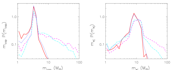
Figure 3.— Mass probability distribution $P(m_{{\rm cap}})$ of the captured companions of the $\sim 3$-$4M_{\odot}$ HVSs (left panel) and mass probability distribution $P(m_{{\rm ej}})$ of the ejected companions of the $\sim 7$-$15M_{\odot}$ captured stars (right panel). The solid (red), dotted (blue), dashed (magenta) and dot-dashed (cyan) lines represent the results obtained from the Unbd-MS0, the Disk-MS0, the Disk-TH0, and the Disk-TH2 models, respectively.

4. Orbital evolution of the captured stars

The orbits of the captured stars produced by the tidal breakup of stellar binaries may evolve due to dynamical interactions with the surrounding environments. In principle, two-body interactions between stars may cause exchanges of their angular momenta and energy. However, the timescale of the two-body relaxation ($\sim 10^{9}$ yr) is too long for it to be effective in changing the orbits of captured stars within their main-sequence lifetime (e.g., Hopman & Alexander, 2006; Yu et al., 2007). The RR is an important dynamical process naturally resulted from the coherent torques between orbital averaged mass wires of stars moving in near-Keplerian potential proposed by Rauch & Tremaine (1996), which can lead to changes in both the eccentricities (scalar RR) and orientations (vector RR) of stars moving in the GC (e.g., Hopman & Alexander, 2006). The RR appears much more effective in changing the orbital configuration of the “GC S-stars” than the non-resonant two-body relaxation (NR; Hopman & Alexander, 2006; Perets et al., 2009; Kocsis & Tremaine, 2011). Therefore, the scalar and vector RR may be crucial in the follow-up dynamical evolution of the orbits of the captured stars.

The vector RR timescale is $\sim 1$-$10$ Myr in the region hosting the “GC S-stars”, about one order of magnitude smaller than the scalar RR timescale (Hopman & Alexander, 2006; Yu et al., 2007), and thus the captured stars can evolve to an isotropic distribution on a timescale of $\sim 10$ Myr (Hopman & Alexander, 2006; Perets et al., 2009; Kocsis & Tremaine, 2011) even if they were originally on a plane-like structure. In this paper, we assume that the isotropic distribution of the GC S-stars can always be reproduced through the vector RR of the simulated captured stars within a timescale shorter than their lifetime. It has been suggested that the high-eccentric orbits of captured stars can dynamically evolve to that of the observed GC S-stars through the scalar RR within $\sim 20$ Myr (e.g., Perets et al., 2009). However, previous studies assume a simple distribution of the initial eccentricities and semimajor axes of the captured stars (e.g., Perets et al., 2009; Madigan et al., 2011). In this Section, we adopt the distribution of $e_{\rm cap}$ and $a_{\rm cap}$ resulted from the injection models studied in Section 3. We follow the evolution of $e_{\rm cap}$ and $a_{\rm cap}$ by taking both the RR and NR into account, and then compare the $e_{\rm cap}$ and $a_{\rm cap}$ distributions of the captured stars surviving to the present time with that of the observed GC S-stars.

We adopt the ARMA model first introduced by Madigan et al. (2011) to perform Monte Carlo simulations of the long-term evolution of the captured stars. In the ARMA model, the RR phase and the NR phase are unified, and the general relativistic (GR) precession of stars in the potential of the central MBH is also simultaneously included. The ARMA model is characterized by the following three parameters: (1) the autoregressive parameter $\phi_{1}$; (2) the moving average parameter $\theta_{1}$; and (3) the parameter $\sigma_{1}$, which is the variance of a random variable $\epsilon^{(1)}$ following the normal distribution. In the ARMA model, $\epsilon^{(1)}$ represents the random walk motion of the NR phase. At a time step of one orbital period of a star, the variation in the absolute value of its angular momentum is

$$\Delta_{1}J_{t}=\phi_{1}\Delta_{1}J_{t-1}+\theta_{1}\epsilon^{(1)}_{t-1}+\epsilon^{(1)}_{t},$$ (12)

and

$$\phi_{1}=\exp{(-\frac{\delta t_{\rm P}}{St_{\phi}})},$$ (13)

$$t_{\phi}=f_{\phi}{\rm min}[t_{\rm prec}(a,e),t_{\rm prec}(a,\tilde{e})],$$ (14)

$$S=\frac{1}{1+\exp{\left[-k\left(e-e_{\rm crit}\right)\right]}},$$ (15)

$$e_{\rm crit}(a,e)=\sqrt{\frac{\ln\Lambda}{A_{\rm NR}A_{\tau}^{2}}}\left(\frac{\delta t_{\rm P}}{t_{\phi}}\right),$$ (16)

$$\theta_{1}=-\exp\left[{-\frac{f_{\theta}}{2}\sqrt{\frac{1}{\phi_{1}^{2}}+\phi^{2}_{1}-2+\frac{4(1-\phi^{2}_{1})\tau^{2}\delta t_{\rm P}^{2}}{\sigma^{2}_{1}}}}\right],$$ (17)

$$\tau=A_{\tau}\frac{m_{*}}{M_{\bullet}}\frac{\sqrt{N_{<}}}{\delta t_{\rm P}}e,$$ (18)

$$\sigma_{1}=f_{\sigma}\frac{m_{*}}{M_{\bullet}}\sqrt{\frac{N_{<}\ln\Lambda}{A_{\rm NR}}},$$ (19)

$$f_{\sigma}=0.52+0.62e-0.36e^{2}+0.21e^{3}-0.29\sqrt{e},$$ (20)

where $f_{\phi}=0.105$, $f_{\theta}=1.2$, $k=30$, $A_{\rm NR}=0.26$, $A_{\tau}=1.57$, $\Lambda=M_{\bullet}/m_{*}$, $m_{*}=10M_{\odot}$ is the averaged mass of the field stars, $a$ and $\delta t_{\rm P}$ are the semimajor axis and orbital period of the star, $\tilde{e}$ is the median value of the eccentricity of the field stars and it is $\sqrt{1/2}$ for a thermal distribution, $t_{\rm prec}$ is the combined precession timescale for the Newtonian precession and the general relativity precession (see Equations (25), (27), and (28) in Madigan et al., 2011), and $N_{<}$ is the total number of stars within the radius equal to the semimajor axis of the captured star. Adopting a simple stellar cusp model, i.e., $\rho_{*}\propto r^{-\alpha}$, we have $N_{<}=N_{\rm h}(r/r_{\rm h})^{3-\alpha}$, where $r_{\rm h}$ represents the radius within which the mass of stars equals the MBH mass and $N_{\rm h}=M_{\bullet}/m_{*}=4\times 10^{5}$ is the total number of field stars within $r_{\rm h}$. Similar to Madigan et al. (2011), we also assume a Bahcall–Wolf cusp ($\alpha=7/4$, Bahcall & Wolf 1976) unless otherwise stated and correspondingly $r_{\rm h}=2.3{\rm~{}pc}$. The variable superscript ‘(1)’ in the above equations means that the time step is one orbital period of the star being investigated. In the time step of $N$ period of the star ($N=\delta t/\delta t_{\rm P}$), the model parameters ($\phi_{N}$, $\theta_{N}$, $\sigma_{N}$) can be obtained from parameters of one period ($\phi_{1}$, $\theta_{1}$, $\sigma_{1}$). For further details of the ARMA model, see Madigan et al. (2011). The ARMA model may not capture the exact dynamical physics of the system and give the exact kinematics of each individual star; but for the purpose of our work and the addressing problems, it should be plausible and efficient to be applied here to obtain the evolution of the system in a statistical way.

The two-body NR is also taken into account in a way similar to that in Madigan et al. (2011). In a time step $\delta t$, the energy change of a captured star due to the NR is given by

$$\Delta E=\xi E\left(\frac{\delta t}{t_{\rm NR}}\right)^{1/2},$$ (21)

where $\xi$ is an independent normal random variable with zero mean and unit variance, and $t_{\rm NR}$ is the NR timescale in the GC given by

$$t_{\rm NR}=A_{\rm NR}\left(\frac{M_{\bullet}}{m_{*}}\right)^{2}\frac{1}{N_{<}}\frac{1}{\ln\Lambda}\delta t_{\rm P}.$$ (22)

The travel time of those HVSs discovered in the Galactic halo is $\sim 40$-$250$ Myr if HVSs were ejected from the GC (Brown et al., 2009a). And recent observations have also shown that the age of the detected HVSs is on the order of $\sim 100$ Myr, which is consistent with the GC origin (Brown et al., 2012a). In the model of this paper, we are unifying the formation of both the HVSs and the GC S-stars by the tidal breakup of young stellar binaries originated from the young stellar disk(s) in the GC. In order to be compatible with the above observations, we assume a constant injection rate of stellar binaries over the past $250$ Myr. We adopt the numerical results of the three-body experiments for each injection model in Section 3 and calculate the energy and angular momentum evolution for each captured star by using the ARMA model. In these calculations, we also take account of the effects of the limited lifetime of the captured stars on the main sequence and the tidal disruption of those captured stars moving too close to the MBH. We remove those captured stars if they move away from the main sequence or approach the MBH within a distance of $r_{\rm p}<r^{\rm td}$, where $r^{\rm td}=(2M_{\bullet}/m)^{1/3}R_{*}$ and $R_{*}$ is the stellar radius. Finally, we obtain the present-day semimajor axis and eccentricity distributions of the captured stars, which can be used to be compared to the observational distributions and constrain the models.

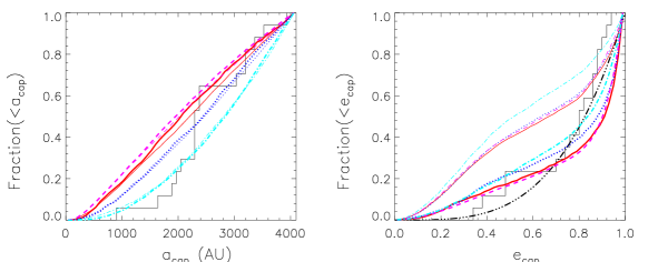
Figure 4.— Cumulative distributions of the semimajor axis (left panel) and eccentricity (right panel) of the captured stars surviving to the present time. The histograms represent the distributions of the observed GC S-stars (Gillessen et al., 2009). The solid (red), dotted (blue), dashed (magenta), and dot-dashed (cyan) curves show the results obtained from the Unbd-MS0 model, the Disk-MS0 model, the Disk-TH0 model, and the Disk-TH2 model, respectively. The thick and thin curves represent the distributions of those captured stars with mass $7$-$15M_{\odot}$ and $3$-$4M_{\odot}$, respectively. In the right panel, the dot-dot-dashed line represents the cumulative eccentricity distribution proportional to $e_{\rm cap}^{3.6}$ as suggested by the observations (Ghez et al., 2008; Gillessen et al., 2009).

The left panel of Figure 4 shows the cumulative distributions of $a_{\rm cap}$ of the captured stars surviving to the present time and that of the observed GC S-stars. The thick lines represent the captured stars with mass $\sim 7$-$15M_{\odot}$ surviving to the present time (the simulated GC S-stars), roughly corresponding to the observed GC S-stars, and the thin lines represent the captured stars with mass $\sim 3$-$4M_{\odot}$, roughly corresponding to the captured companions of those HVSs detected in the Galactic halo. Although the lifetime of less massive stars on the main sequence is substantially longer and thus the dynamical evolution time is longer than that of the massive ones, the cumulative distribution of $a_{\rm cap}$ of the light captured stars is only slightly different from that of the massive ones (see the left panel of Figure 4). The slope of the $a_{\rm cap}$ distribution is affected most by the $f_{r_{\rm p}}(r_{\rm p,ini})$ distribution. Relatively fewer captured stars are produced in the inner region by the Disk-TH2 model compared with that obtained by the other models, and the fraction of captured stars with semimajor axes $<a_{\rm cap}$ is proportional to $\sim a_{\rm cap}^{2.0}$ for the Disk-TH2 model but to $\sim a_{\rm cap}^{1.0-1.5}$ for the other three models. For those models with $\beta=0$, the $a_{\rm cap}$ distributions obtained from the numerical simulations is roughly consistent with the simple estimations from Equation (9) (e.g., the slope is $1$ for $\alpha=-1$ and $\beta=0$ according to Equation (9)). For the Disk-TH2 model, however, the $a_{\rm cap}$ distribution seems flatter than the simple expectation, i.e., a slope of $3$ (for $\alpha=-1$ and $\beta=2$). The flatter slope of $f(a_{\rm cap})$ resulted from the Disk-TH2 model may be due to the effect of various mass ratios of the injecting binaries, which is included in the numerical simulations but ignored in deriving Equation (9) (see panel (d) in Figure (1)). The Kolmogorov–Simirnov (K-S) tests find the likelihoods of $0.02$, $0.2$, $0.05$, and $0.15$ that the $a_{\rm cap}$ distribution of the observed GC S-stars is the same as that of the simulated GC S-stars for the four models, respectively. As shown in Figure 4, most of the discrepancy between the observational distribution and the simulated one is apparently near the edges of those distributions. Since the Anderson–Darling (A-D) test may be more effective than the K-S test and more sensitive to the distribution edges (see Feigelson & Babu, 2012), we also adopt the A-D test here and find the likelihoods are $0.05$, $0.3$, $0.03$, and $0.32$ for the four models, respectively. These statistical tests suggest that the Disk-MS0 model and the Disk-TH2 model may be more compatible with the observational $a_{\rm cap}$ distribution.

For the majority of the simulated GC S-stars ($\sim 7$-$15M_{\odot}$), the relative changes in their energy due to dynamical relaxation after their capture are less than $\sim$30% and their semimajor axes do not deviate much from the initial values right after their capture. Therefore, the distribution of the semimajor axis of currently observed GC S-stars can provide some information on their ejected companions (see Equations (4) and (5)). For those captured stars with mass $\sim 3$-$4M_{\odot}$, however, their relative energy changes can be as large as $1$ mainly because of their longer lifetime and thus longer dynamical evolution time, and Equation (5) is no longer reliable to provide estimations on the velocity of the ejected companions of those less massive captured stars by using their present-day semimajor axes.

The right panel of Figure 4 shows the cumulative eccentricity distributions obtained from different models. As seen from Figure 4, the $e_{\rm cap}$ distributions are only slightly different for different injection models because the initial $e_{\rm cap}$ are all close to $1$ in all the models. For those captured stars with mass $\sim 3$-$4M_{\odot}$, their present eccentricities are relatively lower than that of the observed GC S-stars because of their longer dynamical evolution time. For those simulated GC S-stars (with mass $\sim 7$-$15M_{\odot}$) resulted from any of the four injection models, their $e_{\rm cap}$ distribution is similar to that of the observed GC S-stars. The K-S tests find a likelihood of $\sim 0.1-0.6$ that the eccentricity distribution of the observed S-stars is the same as that of the simulated GC S-stars for all the four models. If alternatively adopting the A-D test, then the likelihoods are $\sim 0.004,0.02,0.005$, and $0.13$ for the Unbd-MS0 model, the Disk-MS0 model, the Disk-TH0 model, and the Disk-TH2 model, respectively. According to these calculations, the Disk-TH2 model may be more compatible with the observational $e_{\rm cap}$ distribution.

We note here that the simulations slightly over-produce the stars with high eccentricities ($e_{\rm cap}$ close to $1$) with respect to the observations because the RR for those captured stars with extremely high eccentricities is quenched by the strong relativistic precession (Madigan et al., 2011). For this inconsistency, part of the reason might be the observational bias in detecting the GC S-stars, i.e., the stars with high eccentricities are less likely to be detected at $a_{\rm cap}\sim 0.01{\rm~{}pc}$ (Schödel et al., 2003; Weinberg et al., 2005; Madigan et al., 2011); and part of the reason might be the limitation of the ARMA model. But the main reason of the inconsistency does not appear to be due to ignoration of the “bouncing effect” demonstrated in Figure 7 of Merritt et al. (2011), where the star starting from a low-eccentricity orbit and evolving close to a critical high-eccentricity orbit is then bounced back onto a low-eccentricity orbit due to the suppression of the RR by the fast GR precession at high-eccentricity orbits, as (1) the stars in our model are captured from tidal breakup of binary stars and they initially have eccentricities even higher than the critical eccentricities; (2) during the simulation period, some of the stars have evolved onto low-eccentricity orbits as illustrated by the distribution at the low-eccentricity end in Figure 4, and the simulated stars at the high-eccentricity end are those that evolve relatively slowly; and (3) the suppression of the RR due to the fast GR precession has been modeled in our work, as mentioned before (e.g., see the definition of $t_{\rm prec}$ above).

The timescale of the RR process also depends on the mass of the field stars (Madigan et al., 2011; Rauch & Tremaine, 1996). To check this dependence, we perform additional simulations by setting the mass of field stars to $m_{*}=5M_{\odot}$ or $m_{*}=20M_{\odot}$ but with the total mass of the field stars fixed. According to the results of these simulations, we find that the simulated GC S-stars are on orbits with too high eccentricities compared with the observational ones if $m_{*}=5M_{\odot}$, or on orbits with too low eccentricities if $m_{*}=20M_{\odot}$.

In the above calculations, a Bahcall–Wolf cusp for the background stellar system in the GC is adopted. However, recent observations suggested that the background stellar distribution may be core-like rather than cusp-like (e.g., Do et al. 2009). Similarly as done in Madigan et al. (2011), we also adopt $\alpha=0.5$ to mimic the effect of a core-like distribution, and the perturbation on the GC “S-stars” is assumed to be dominated by main-sequence stars (e.g., see Antonini & Merritt 2012). In such a model, we find that the resulted S-stars on highly eccentric orbits with smaller pericenter distances are relatively more than those obtained from the cuspy model. The reason is that the RR is less efficient in the core-like stellar distribution, and thus the evolution of the eccentricities of GC “S-stars” is slower.

The timescale of the RR process becomes much longer at the distance of the disks. Stars in this region are less affected by the relaxation processes and may well preserve some of their initial orbital configurations. Observations find many B-dwarfs in disk regions, with high eccentricities and more extended spatial distribution than disk stars. The resulted eccentricity–distance distribution of these stars by the RR compared with the observations may provide useful constraints on the formation of the GC S-stars (Perets et al., 2010). Our simulations also produce many B-dwarfs in the disk region and their radial distribution is similar to the initial input ones for the injecting binaries. However, there should also exist B-dwarfs in the disk region that are initially formed as single stars and the fraction of these stars is not clear yet. A detailed dynamical study for the B-dwarfs in the disk region is complicated and beyond the scope of this paper.

5. Ejected HVSs in the Galactic bulge and halo

The ejected stars move away from the GC after the breakup of their progenitor binaries and their velocities are gradually decelerated in the Galactic gravitational potential. Some of them are unbound to the Galactic potential and can travel to the Galactic halo and may appear as the detected HVSs if their main-sequence lifetime is long enough compared to the travel time; while others with lower ejecting velocity may return to the GC. To follow the subsequent motion of the ejected components, we adopt the Milky Way potential model given by Xue et al. (2008), which involves four components, including the contributions from the central MBH, the Galactic bulge, the Galactic disk, and the Galactic halo, i.e.,

$$\Phi=\Phi_{\rm BH}+\Phi_{\rm bulge}+\Phi_{\rm disk}+\Phi_{\rm halo},$$ (23)

where

$$\Phi_{\rm BH}=-GM_{\bullet}/r,$$ (24)

$$\Phi_{\rm bulge}=-\frac{GM_{\rm bulge}}{r+r_{\rm bulge}},$$ (25)

$$\Phi_{\rm disk}=-\frac{GM_{\rm disk}(1-e^{-r/b})}{r},$$ (26)

$$\Phi_{\rm halo}=-\frac{4\pi G\rho_{\rm s}r^{3}_{\rm vir}}{c^{3}r}\ln(1+\frac{cr}{r_{\rm vir}}),$$ (27)

respectively. The model parameters for the last three components are $M_{\rm bulge}=1.5\times 10^{10}M_{\odot}$, $M_{\rm disk}=5\times 10^{10}M_{\odot}$, the core radius $r_{\rm bulge}=0.6\rm~{}kpc$, the scale length $b=4\rm~{}kpc$, and $\rho_{\rm s}=\frac{1}{3}\frac{c^{3}\rho_{\rm c}\Omega_{\rm m}\Delta_{\rm vir}}{\ln(1+c)-c/(1+c)}$, where $\rho_{\rm c}$ is the cosmic critical density, $\Delta_{\rm vir}=200$, $\Omega_{\rm m}$ is the cosmic fraction of matter, the virial radius $r_{\rm vir}=267\rm~{}kpc$, and the concentration $c=12$. The bulge, the disk, and the halo potentials adopted here are all spherical. If adopting non-spherical potentials, i.e., a triaxial bulge/halo and a flattened disk potential, the bending effect due to the non-spherical component on the trajectories of ejected stars is important only for those with $v_{\infty}\mathrel{\mathchoice{\lower 4.0pt\vbox{\halign{$\nms\displaystyle\hfil#\hfil$\cr<\crcr\sim\crcr}}}{\lower 4.0pt\vbox{\halign{$\nms\textstyle\hfil#\hfil$\cr<\crcr\sim\crcr}}}{\lower 4.0pt\vbox{\halign{$\nms\scriptstyle\hfil#\hfil$\cr<\crcr\sim\crcr}}}{\lower 4.0pt\vbox{\halign{$\nms\scriptscriptstyle\hfil#\hfil$\cr<\crcr\sim\crcr}}}}400{\rm km\,s^{-1}}$ on a timescale of $\mathrel{\mathchoice{\lower 4.0pt\vbox{\halign{$\nms\displaystyle\hfil#\hfil$\cr>\crcr\sim\crcr}}}{\lower 4.0pt\vbox{\halign{$\nms\textstyle\hfil#\hfil$\cr>\crcr\sim\crcr}}}{\lower 4.0pt\vbox{\halign{$\nms\scriptstyle\hfil#\hfil$\cr>\crcr\sim\crcr}}}{\lower 4.0pt\vbox{\halign{$\nms\scriptscriptstyle\hfil#\hfil$\cr>\crcr\sim\crcr}}}}500$ Myr, but it is negligible for HVSs with relatively high speeds (see Yu & Madau, 2007). Note that the radial distribution of the ejected stars surviving to the present time (and correspondingly the predicted number of the detectable HVSs) may be slightly different if adopting a different Galactic potential model.

The total number of detectable HVSs depends directly not only on how many stellar binaries can be injected into the immediate vicinity of the MBH, but also on the lifetime of these stars and the detailed settings on the IMF, semimajor axis, and periapsis of the injecting stellar binaries (see Section 3). If the stellar binaries are injected from a far away region, the injection rate can be estimated through the loss-cone theory (Yu & Tremaine, 2003; Perets et al., 2009); if the injecting stellar binaries originated from central stellar disks (Lu et al., 2010; Zhang et al., 2010), the injection rate is difficult to estimate as the mechanism responsible for it is still not clearly understood (cf. Madigan et al. 2009). In principle, it is plausible to observationally calibrate the injection rate by the numbers of the detected HVSs and GC S-stars. But this calibration becomes complicated if considering of the uncertainties in the settings of the distributions $f_{a_{\rm b}}(a_{\rm b,ini})$, $f_{r_{\rm p}}(r_{\rm p,ini})$, and IMF of the injecting binaries, etc.

Table 3The Number Ratio of the Simulated $3$-$4M_{\odot}$ HVSs to the Simulated GC S-stars

Model	$\gamma$	$\beta$	$\frac{N_{{\rm HVS}}^{{\rm tot}}}{N_{{\rm cap}}^{{\rm tot}}}$	$\frac{F^{{\rm lt}}_{{\rm HVS}}}{F^{{\rm lt}}_{{\rm cap}}}$	$F^{\rm td}_{{\rm cap}}$	$F_{\rm HVS}^{\rm obs,rf}$	$F_{{\rm cap}}^{\rm obs}$	$\frac{N_{\rm HVS}^{\rm obs,rf}}{N_{{\rm cap}}^{\rm obs}}$
Unbd-MS0	-2.7	0	3.0	8.8	0.59	0.27	0.51	27
Disk-MS0	-2.7	0	1.8	8.9	0.51	0.15	0.41	12
Disk-TH0	-0.45	0	0.22	10	0.47	0.19	0.54	1.4
Disk-TH2	-0.45	2	0.27	9.9	0.34	0.06	0.21	1.3
Disk-IM0	-1.6	0	0.61	9.5	0.50	0.16	0.47	4.0
Disk-IM2	-1.6	2	0.75	9.4	0.22	0.01	0.03	2.8

Note. — The $N_{\rm HVS}^{{\rm tot}}$ and $N_{{\rm cap}}^{{\rm tot}}$ represent the total number of the ejected stars with mass $3$-$4M_{\odot}$ and the total number of the captured stars with mass $7$-$15M_{\odot}$ that are generated by the tidal breakup of stellar binaries in the GC for each model, respectively; the $F^{{\rm lt}}_{\rm HVS}$ and $F^{{\rm lt}}_{{\rm cap}}$ denote the fraction of the ejected and captured stars that still remain on the main sequence of their stellar evolution at the end of our simulations; the $F^{\rm td}_{{\rm cap}}$ denotes the fraction of the captured stars that have been tidally disrupted by the central MBH before the end of our simulations; the $F_{\rm HVS}^{\rm obs,rf}$ denotes the fraction of the ejected stars appear as the detected HVSs, where an ejected star is taken as a detectable HVS if its heliocentric radial velocity in the Galactic rest frame is $|v_{\rm rf}|>275{\rm km\,s^{-1}}$, its velocity at infinity is $v_{\infty}>750{\rm km\,s^{-1}}$, and its distance from the GC is in the range of $40$-$130\rm~{}kpc$; $F_{{\rm cap}}^{\rm obs}$ denotes the fraction of the captured stars that are within radii $\mathrel{\mathchoice{\lower 4.0pt\vbox{\halign{$\nms\displaystyle\hfil#\hfil$\cr<\crcr\sim\crcr}}}{\lower 4.0pt\vbox{\halign{$\nms\textstyle\hfil#\hfil$\cr<\crcr\sim\crcr}}}{\lower 4.0pt\vbox{\halign{$\nms\scriptstyle\hfil#\hfil$\cr<\crcr\sim\crcr}}}{\lower 4.0pt\vbox{\halign{$\nms\scriptscriptstyle\hfil#\hfil$\cr<\crcr\sim\crcr}}}}4000{\rm AU}$ from the MBH; and the $N_{\rm HVS}^{\rm obs,rf}$ is the total number of those detectable HVSs with mass $3$-$4M_{\odot}$ in the Galactic halo and $N_{{\rm cap}}^{\rm obs}$ is the simulated number of the captured stars with mass $7$-$15M_{\odot}$ in the GC, which correspond to the observed ones.

Table 4Predicted Numbers in Different Models

Model	$\gamma$	$\beta$	injection rate		$3$-$4M_{\odot}$				$4$-$7M_{\odot}$				$7$-$15M_{\odot}$
			$(10^{-5}\,{\rm yr^{-1}})$		$N_{\rm HVS}^{\rm obs,rf}$	$N_{\rm HVS}^{\rm obs,pm}$	$N_{{\rm cap}}^{\rm obs}$		$N_{\rm HVS}^{\rm obs,rf}$	$N_{\rm HVS}^{\rm obs,pm}$	$N_{{\rm cap}}^{\rm obs}$		$N_{\rm HVS}^{\rm obs,rf}$	$N_{\rm HVS}^{\rm obs,pm}$	$N_{{\rm cap}}^{\rm obs}$
Unbd-MS0	-2.7	0	13 (2.2)		504 (79)	189 (30)	86 (13)		178 (28)	58 (9)	33 (5)		60 (9)	33 (5)	17 (3)
Disk-MS0	-2.7	0	7.0 (2.7)		177 (79)	66 (29)	82 (36)		62 (28)	21 (9)	32 (14)		29 (13)	17 (8)	17 (8)
Disk-TH0	-0.45	0	1.8 (5.8)		23 (79)	8 (27)	11 (37)		28 (97)	8 (30)	11 (39)		29 (103)	19 (66)	17 (60)
Disk-TH2	-0.45	2	6.2 (23)		18 (79)	7 (31)	8 (34)		16 (71)	5 (23)	9 (40)		20 (87)	15 (64)	17 (75)
Disk-IM0	-1.6	0	3.1 (3.6)		61 (79)	22 (29)	28 (36)		37 (48)	12 (15)	18 (23)		29 (38)	18 (23)	17 (22)
Disk-IM2	-1.6	2	60 (100)		48 (79)	21 (35)	32 (52)		24 (39)	7 (11)	18 (29)		20 (33)	14 (23)	17 (28)

Note. — The numbers of the simulated detectable HVSs and the captured stars surviving in the GC at the present time in different mass ranges, obtained from different models. The injection rate of stellar binaries is assumed to be a constant over the past $250$ Myr, which enables the production of $17$ simulated GC S-stars (or $79$ unbound $3\sim 4M_{\odot}$ HVSs (numbers in the brackets)). The $N_{\rm HVS}^{\rm obs,rf}$ denotes the number of HVSs with $|v_{\rm rf}|>275{\rm km\,s^{-1}}$ and $v_{\infty}>750{\rm km\,s^{-1}}$; and the $N_{\rm HVS}^{\rm obs,pm}$ denotes the number of the HVSs with proper motion $\geq 5{\rm mas\,yr^{-1}}$ in the heliocentric rest frame and $v_{\infty}>750{\rm km\,s^{-1}}$. In order to compare to the observations, a simulated HVS with mass of $3$-$4M_{\odot}$ is counted as a detectable HVS additionally if its distance to the GC is in the range of $40-130\rm~{}kpc$. The $N_{{\rm cap}}^{\rm obs}$ is the total number of the captured stars surviving in the GC with present-day $a_{\rm cap}\mathrel{\mathchoice{\lower 4.0pt\vbox{\halign{$\nms\displaystyle\hfil#\hfil$\cr<\crcr\sim\crcr}}}{\lower 4.0pt\vbox{\halign{$\nms\textstyle\hfil#\hfil$\cr<\crcr\sim\crcr}}}{\lower 4.0pt\vbox{\halign{$\nms\scriptstyle\hfil#\hfil$\cr<\crcr\sim\crcr}}}{\lower 4.0pt\vbox{\halign{$\nms\scriptscriptstyle\hfil#\hfil$\cr<\crcr\sim\crcr}}}}4000{\rm AU}$ in the simulations.

5.1. The Numbers of the HVSs/GC S-stars and Their Number Ratio

The $3$-$4M_{\odot}$ HVSs detected in the Galactic halo and the GC S-stars should be linked to each other under the working hypothesis of this paper. The total numbers of the simulated $3$-$4M_{\odot}$ HVSs and $7$-$15M_{\odot}$ GC S-stars depend not only on the injection rate of stellar binaries but also on the detailed settings on the injection models. However, the number ratio of the simulated $3$-$4M_{\odot}$ HVSs to the simulated $7$-$15M_{\odot}$ GC S-stars may depend only on the details of the injection models described in Section 3, but not on the injection rate of stellar binaries. Any viable model should produce a number ratio compatible with the observations on the HVSs and the GC S-stars, and thus this number ratio may provide important constraints on the models.

We obtain both the numbers of the simulated HVSs and the captured stars surviving to the present time and their number ratio by Monte Carlo simulations as follows. First, we obtain the total number of initially captured (or ejected) stars, $N_{{\rm cap}}^{{\rm tot}}$ (or $N_{{\rm HVS}}^{{\rm tot}}$), with mass in the ranges of $3$-$4M_{\odot}$, $4$-$7M_{\odot}$, and $7$-$15M_{\odot}$, respectively. To do this, we assume a constant injection rate of binaries and randomly set the injection events over the past $250$ Myr, and for each injection event we randomly assign it to a three-body experiment conducted in Section 3 and adopt the results from the experiment. Second, we consider the limited lifetime of each ejected and captured star, the motion of each ejected star in the Galactic potential, and the dynamical evolution of each captured star, and then obtain the fraction of the ejected stars ($F_{\rm HVS}^{{\rm lt}}$) that still remain on the main sequence at the present time or the similar fraction for the captured stars ($F_{{\rm cap}}^{{\rm lt}}$), and the fraction of the captured stars ($F_{{\rm cap}}^{\rm td}$) that have already been tidally disrupted until the present time. Third, we consider the kinematic selection criteria and obtain the fractions of those ejected and captured stars according to given observational selection criteria, i.e., $F_{\rm HVS}^{\rm obs}$ and $F_{{\rm cap}}^{\rm obs}$, respectively. The selection criteria are similar to those adopted in selecting the detected HVSs and GC S-stars, i.e., an ejected star is labeled as a detectable HVS if its heliocentric radial velocity in the Galactic rest frame is $|v_{\rm rf}|>275{\rm km\,s^{-1}}$ or its proper motion in the heliocentric rest frame is $\geq 5{\rm mas\,yr^{-1}}$, and its velocity at infinity is $v_{\infty}>750{\rm km\,s^{-1}}$, and captured stars with semimajor axis $\mathrel{\mathchoice{\lower 4.0pt\vbox{\halign{$\nms\displaystyle\hfil#\hfil$\cr<\crcr\sim\crcr}}}{\lower 4.0pt\vbox{\halign{$\nms\textstyle\hfil#\hfil$\cr<\crcr\sim\crcr}}}{\lower 4.0pt\vbox{\halign{$\nms\scriptstyle\hfil#\hfil$\cr<\crcr\sim\crcr}}}{\lower 4.0pt\vbox{\halign{$\nms\scriptscriptstyle\hfil#\hfil$\cr<\crcr\sim\crcr}}}}4000{\rm AU}$ are counted as detectable GC S-stars. For those simulated HVSs with mass $3$-$4M_{\odot}$, we put an additional cut on their distances from the GC, i.e., from $40$ to $130\rm~{}kpc$, in order to compare them to current observations. Finally, we obtain the number ratio of the detectable HVSs to the detectable GC S-stars for each model as

$$\frac{N_{\rm HVS}^{\rm obs}}{N_{{\rm cap}}^{\rm obs}}=\frac{N_{{\rm HVS}}^{{\rm tot}}}{N_{{\rm cap}}^{{\rm tot}}}\times\frac{F^{\rm lt}_{{\rm HVS}}}{F^{{\rm lt}}_{{\rm cap}}}\times\frac{F_{\rm HVS}^{\rm obs}}{(1-F^{\rm td}_{{\rm cap}}){F_{{\rm cap}}^{\rm obs}}}.$$ (28)

The simulation results are listed in Tables 3 and 4 for each model.

Here we comment on a few factors that affect the predicted numbers of the simulated detectable HVSs and GC S-stars and consequently the number ratio of these two populations. (1) The difference between the lifetime of the simulated HVSs and GC S-stars: the detected HVSs are in the mass range of $\sim 3$-$4M_{\odot}$, which are substantially smaller than that of the observed GC S-stars ($\sim 7$-$15M_{\odot}$). The lifetime difference leads to an enhancement in the number ratio of the detectable HVSs to the GC S-stars roughly by a factor of $10$ under the assumption of a constant rate of injecting stellar binaries into the vicinity of the MBH over the past $250$ Myr. (2) The place where the stellar binaries are originated: in the Unbd-MS0 model, relatively more stars with high velocities (e.g., $>1000{\rm km\,s^{-1}}$) are generated than those in the other models. (3) The distribution of pericenter distance of those injecting stellar binaries, which is related to the speed of the migration or diffusion process of those binaries to the immediate vicinity of the central MBH: a change in this distribution may result in either a significant increase or decrease in both the number of HVSs and that of captured stars, but their number ratio is not affected much.

The complete survey conducted by Brown et al. (2009a) has detected $14$ unbound HVSs with mass $\sim 3$-$4M_{\odot}$ in a sky area of $\sim 7300$ deg², and the total number of similar HVSs in the whole sky should be $\sim 79\pm 21$. Observations have revealed $17$ GC S-stars within a distance of $\sim 4000{\rm AU}$ from the central MBH. The number ratio of the detected HVSs to the GC S-stars is $\sim 3.4$-$5.9$. The number ratio resulted from any of the top four injection models listed in Table 2 is inconsistent with the observational ones. Both the Unbd-MS0 model and the Disk-MS0 model give a number ratio substantially larger than that inferred from observations, while the Disk-TH0 model and the Disk-TH2 model give too small number ratios.

Figer et al. (1999) suggest that the IMF of young star clusters in the GC, i.e., the Arches cluster, may be top-heavy and the IMF slope is $\gamma\sim-1.6$, although some later studies argued that the IMF of Arches cluster may be still consistent with the Salpeter one by assuming continuous star formation (e.g., Löckmann et al., 2010). Considering of this, we adopt an IMF with a slope of $\gamma=-1.6$ and perform two additional injecting models, i.e., “Disk-IM0” and “Disk-IM2”, as listed in Tables 3 and 4. Our calculations show that the number ratios produced by the two models are close to the observational ones. Obviously, the number ratio of the simulated HVSs to GC S-stars is significantly affected by the adopted IMF. Adopting a steeper IMF may lead to a larger number ratio.

The velocity distribution of the detected HVSs suggests a slow migration/diffusion of stellar binaries into the immediate vicinity of the central MBH (see detailed discussions in Zhang et al., 2010). The Disk-IM2 model can produce a velocity distribution similar to the observational ones, and the large $\beta$ adopted in this model also suggests a slow migration/diffusion of binaries into the vicinity of the central MBH. However, all the other models appear to generate too many HVSs at the high-velocity end and thus a too flat velocity distribution compared with the observational ones. This inconsistency could be due to many factors. For example, (1) the velocity distribution of the detected HVSs could be biased due to either the small number statistics and/or the uncertainties in estimating the observational selection effects; (2) the uncertainties in the initial settings of the injecting binaries could also lead to some change in the velocity distribution, e.g., the velocity distribution may be steeper if the semimajor axis distribution of stellar binaries is log-normal, rather than follow the Öpik law (Sesana et al., 2007; Zhang et al., 2010); and (3) the injection of binaries to the vicinity of the central MBH may be quite different from the simple models adopted in this paper because of the complicated environment of the very central region, e.g., the possible existence of a number of stellar-mass BHs or an intermediate-mass black holes (BHs) within $100{\rm AU}$.

For each model, the injection rate of stellar binaries can be calibrated to produce the numbers of the observed HVSs and GC S-stars. Under the initial settings for each model described in Section 3, the numbers of the simulated HVSs and the GC S-stars, similar to the detected ones, are listed in Table 4. The calibrated injection rates are also listed in Table 4 for each model and they are roughly on the order of $\sim 10^{-3}$ to $10^{-5}~{}{\rm yr}^{-1}$. However, one should be cautious about that this injection rate depends on the initial settings on the distributions of the semimajor axes and the periapses of the injecting binaries. According to our simulations, many of the injected binaries are not tidally broken up, and the breakup rate is a factor of $3$-$6$ times smaller than the injection rate for those models studied in this paper, i.e., about a few times $10^{-4}$ to $10^{-5}~{}{\rm yr}^{-1}$, which is consistent with the estimates by Bromley et al. (2012).

5.2. The Ejected Companions of the GC S-stars

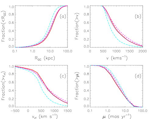
Figure 5.— Cumulative distributions of the Galactocentric distance $R_{\rm GC}$ (panel (a)), the velocity in the Galactocentric rest frame (panel (b)), the heliocentric radial velocity in the Galactic rest frame (panel (c)), and the proper motion in the heliocentric rest frame (panel (d)), of those simulated unbound HVSs ($v_{\infty}>750{\rm km\,s^{-1}}$) that were initially associated with the “GC S-stars”. The solid (red), dotted (blue), dashed (magenta), and dot-dashed (cyan) curves are for the Unbd-MS0 model, the Disk-MS0 model, the Disk-TH0 model, and the Disk-TH2 model, respectively.

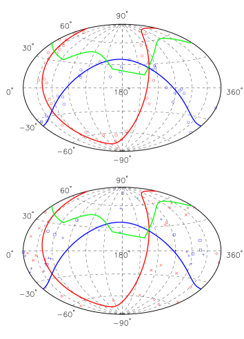
Figure 6.— Spatial distribution of the simulated unbound HVSs with mass $7$-$15M_{\odot}$ and $v_{\infty}>750{\rm km\,s^{-1}}$ for the Disk-IM2 model. The distribution is expressed by a Hammer-Aitoff projection in the Galactic coordinates. In the top panel, the positions of the HVSs are projected to infinity from the GC. The solid red and blue curves represent the CWS and NARM disk planes, respectively, which are also projected to infinity. The region above the green curve shows the area surveyed by Brown et al. (2009a) in the northern hemisphere. The open red and blue circles represent the unbound HVSs originated from binary stars on the CWS and NARM disk planes, respectively. For illustration purpose, all the $34$ simulated HVSs are shown in the top panel (see Table 4). The injection rates are assumed to be the same for the injections from the CWS and the NARM planes and thus the number of HVSs associated with the two planes are also the same. In the bottom panel, the positions of the HVSs are not projected to infinity. The solid red curves and the solid green curve are the same as those for the top panel. The red crosses and blue plus symbols represent those unbound HVSs with $|v_{\rm rf}|\geq 275{\rm km\,s^{-1}}$ injected from the CWS and NARM disk planes, respectively. The red open diamonds and the blue open squares represent the unbound HVSs with proper motion $\mu>5{\rm mas\,yr^{-1}}$ injected from the CWS and the NARM disk planes, respectively.

The HVSs discovered in the Galactic halo are typically in the mass range $\sim 3$-$4M_{\odot}$. HVSs with other masses should also be populated in the Galactic bulge and halo. In this Section, we investigate the properties of the simulated HVSs with mass $\sim 7$-$15M_{\odot}$, which are most likely to be the companions of the “GC S-stars”.

Panel (a) of Figure 5 shows the cumulative distribution of the Galactocentric distances of the high-mass ($\sim 7$-$15M_{\odot}$) HVSs. The predicted numbers of these HVSs from different models are listed in Table 4. The total number of the simulated unbound HVSs, as companions of the population of the GC S-stars, is $\sim 20$-$30$ according to the Disk-IM2 model, which is able to reproduce the numbers of the observed HVSs and GC S-stars. The majority of these unbound HVSs are at distances of a few to a few tens $\rm~{}kpc$ from the GC, which are much closer to the GC than the detected $3$-$4M_{\odot}$ HVSs mainly because a high-mass star has a shorter main-sequence lifetime and thus the distance it can travel within the lifetime is small. The close distances of these HVSs from the GC suggest that the velocity vectors of many of them are not along our line of sight. Their three-dimensional velocities range from $500{\rm km\,s^{-1}}$ to $2000{\rm km\,s^{-1}}$ in the Galactocentric rest frame (see panel (b) in Figure 5); and their heliocentric radial velocities in the Galactic rest frame range from $-500{\rm km\,s^{-1}}$ to $1500{\rm km\,s^{-1}}$ (see panel (c) in Figure 5), where the negative and positive velocities represent moving toward and away from the Sun, respectively. Compared with the ejection velocities of the $3$-$4M_{\odot}$ HVSs, those of the $7$-$15M_{\odot}$ HVSs are relatively higher because of their higher mass (see Equation (1)). Most of the HVSs have proper motions in the heliocentric rest frame as large as ${\rm mas\,yr^{-1}}$ to a few tens ${\rm mas\,yr^{-1}}$ (see panel (d) in Figure 5). These HVSs are bright enough to be detected at a distance less than a few tens $\rm~{}kpc$ by future telescopes, such as, the Global Astrometric Interferometer for Astrophysics spacecraft (Gaia), and their proper motions are also large enough to be measured.

Figure 6 shows the sky distribution of the simulated HVSs with mass$\sim 7$-$15M_{\odot}$, which may represent the ejected companions of the “GC S-stars”, in the Galactic coordinates by a Hammer Aitoff projection. In the top panel of Figure 6, the positions of the HVSs are projected to infinity from the GC, which are consistent with being located close to the CWS disk plane and the Narm plane (also projected to infinity) as expected. In the bottom panel of Figure 6, the positions of the HVSs are not projected to infinity. As seen from the bottom panel, the simulated HVSs with mass $\sim 7$-$15M_{\odot}$ lie in the area below the projected curves of the CWS disk plane and the Narm plane, and most of these high-mass HVSs reside out of the area surveyed by Brown et al. (2009b). Our calculations show that less than $10\%$ of the simulated unbound HVSs with mass $7\sim 15M_{\odot}$ are located in the survey area. This may be the reason that none of those high-mass HVSs, possibly the companions of the “GC S-stars”, has been discovered in the survey area. If the HVSs are initially originated from the CWS disk and the Narm plane, the HVSs with high radial velocities are also relatively rare in the direction close to the disk normals, i.e., $(l,b)=(311{{}^{\circ}},-14{{}^{\circ}})$ and ($176{{}^{\circ}},-53{{}^{\circ}}$) while the HVSs with high proper motions ($\sim 20{\rm mas\,yr^{-1}}$) is relatively numerous in that direction because the velocity vectors of HVSs are close to be perpendicular to the disk normals. Surveys of HVSs in the southern sky with SkyMapper and others may find such massive HVSs, as the possible companions of the “GC S-stars”, and provide crucial evidence for whether those GC S-stars are produced by the tidal breakup of stellar binaries.

Note that the spatial distribution of the HVSs discussed in this section is directly related to the assumption that the injecting stellar binaries are originated from two disk-like stellar structures similar to the CWS disk in the GC. However, the other properties of the HVSs or the GC S-stars discussed in this paper are affected by whether the injecting stellar binaries are bound to the central MBH or not, but not affected by whether they are initially on the CWS disk plane or not.

6. The innermost captured star

The Unbd-MS0, Disk-MS0, Disk-TH0, Disk-TH2, Disk-IM0, and Disk-IM2 models roughly produce $147$, $111$, $21$, $18$, $52$, and $46$ captured stars surviving to the present time and with mass in the range of $3$-$7M_{\odot}$, less massive than that of the GC S-stars, within a distance of $\sim 4000{\rm AU}$ from the MBH (see Table 4 and Section 5). The above numbers are obtained by calibrating the injection rate of the stellar binaries over the past $250$ Myr to generate $17$ simulated GC S-stars similar to the observational number. The captured stars with mass in the range of $3$-$7M_{\odot}$ could be detected by the next generation telescopes, e.g., the Thirty Meter Telescope (TMT) or the European Extremely Large Telescope (E-ELT). These low-mass stars are potentially important probes for testing the GR effects near an MBH, if they are closer to the central MBH than S2. In this section, we estimate the probability distribution of the innermost captured low-mass stars ($\sim 3$-$7M_{\odot}$) by Monte Carlo realizations based on the calibrated injection rate.

The left panel of Figure 7 shows the probability distributions of the semimajor axis of the innermost captured star with mass $\sim 3$-$7M_{\odot}$ resulted from different injection models. For those models adopting $\beta=0$, the resulted innermost captured star is typically on an orbit with semimajor axis $\sim 300{\rm AU}$, and the probability that its semimajor axis is less than that of S2 is $\sim 99\%$. For the other models adopting $\beta=2$, the resulted innermost captured star is on an orbit with semimajor axis of $\sim 300$-$1500{\rm AU}$ and the probability that its semimajor axis is smaller than that of S2 is $\sim 60\%$-$70\%$. The probability to capture a star within the orbit of S2 is larger for the $\beta=0$ models than for the $\beta=2$ models. The reason is that relatively more stellar binaries can be injected into the immediate vicinity of the central MBH and thus more stars can be captured onto orbits with smaller semimajor axes (see Table 4) in the models adopting $\beta=0$ than that adopting $\beta=2$. We conclude that the probability of a less massive star ($3$-$7M_{\odot}$) existing within the S2 orbit is at least $61\%$ and can be up to $99\%$, which may be revealed by future observations and then offer important tests to general relativity.

The right panel of Figure 7 shows the probability distribution of the pericenter distance of the innermost captured low-mass star ($\sim 3$-$7M_{\odot}$) resulted from different injection models. For the injection models adopting $\beta=0$, the pericenter distance distribution is concentrated within $50{\rm AU}$; while for the other models adopting $\beta=2$, the expected pericenter distance is broadly distributed over 10–200 AU. Nevertheless, the probability that the pericenter distance of the innermost captured star with mass $\sim 3$-$7M_{\odot}$ is less than that of S2 (and S14) is still significant, i.e., $\mathrel{\mathchoice{\lower 4.0pt\vbox{\halign{$\nms\displaystyle\hfil#\hfil$\cr>\crcr\sim\crcr}}}{\lower 4.0pt\vbox{\halign{$\nms\textstyle\hfil#\hfil$\cr>\crcr\sim\crcr}}}{\lower 4.0pt\vbox{\halign{$\nms\scriptstyle\hfil#\hfil$\cr>\crcr\sim\crcr}}}{\lower 4.0pt\vbox{\halign{$\nms\scriptscriptstyle\hfil#\hfil$\cr>\crcr\sim\crcr}}}}55\%$ (or $38\%$). The innermost captured star may have its semimajor axis and pericenter distance both significantly smaller than those of S2, therefore, the GR effects on its orbit may be much more significant than that on S2.

If taking into account the captured stars with even lower masses, e.g., $1M_{\odot}$, the number of the expected captured stars surviving to the present time becomes much larger, especially for those models with large $\gamma$. For example, the numbers of the captured stars with mass 1–7$M_{\odot}$ are $907$, $841$, $49$, $39$, $214$, and $117$ for the six models, respectively. For those lower mass captured stars, the semimajor axis and the pericenter of the innermost one could be even closer to the central MBH.

Some stars may be transported to the vicinity of the central MBH by some mechanisms other than the tidal breakup of stellar binaries. It is possible that some of these stars, with their origins different from the captured stars discussed above, exist within the S2 orbit, but which is beyond the scope of the study in this paper.

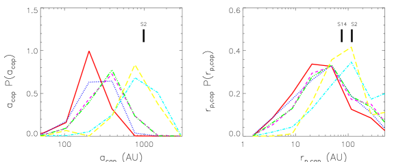
Figure 7.— Probability distributions of the semimajor axis (left panel, $P(a_{{\rm cap}})$) and the pericenter distance (right panel, $P(r_{\rm p,cap})$) of the innermost captured star with mass in the range $\sim 3$-$7M_{\odot}$ (lower than the masses of the GC S-stars) at the present time. The solid (red), dotted (blue), short-dashed (magenta), dot-dashed (cyan), triple -dot-dashed (green), and long-dashed (yellow) lines show the results obtained from the Unbd-MS0, Disk-MS0, Disk-TH0, Disk-TH2, Disk-IM0, and Disk-IM2 models, respectively. Note here that these probability functions rely on the estimation of the numbers of the simulated detectable captured stars (see Section 5). The estimates are obtained by calibrating the injection rate of stellar binaries over the past $250$ Myr to generate the same number (17) of simulated GC S-stars surviving to the present time as that of the observed ones. For reference, the position of S2 (or S14) is labeled in the figure. The probabilities that the innermost star is located within the S2 orbit (i.e., $a_{\rm cap}<1000$AU) are $0.99$, $0,99$, $0.99$, $0.61$, $0.99$, and $0.73$ for the six models, respectively. And the probabilities that the pericenter distance of the inner most star is smaller than that of S2 (S14), i.e., 120 AU (76 AU), are $0.86$ ($0.83$), $0.81$ ($0.75$), $0.78$ ($0.70$), $0.55$ ($0.38$), $0.80$ ($0.70$), and $0.62$ ($0.46$) for the six models, respectively.

7. Conclusions

In this paper, we investigate the link between the GC S-stars and the HVSs discovered in the Galactic halo under the hypothesis that they are both the products of the tidal breakup processes of stellar binaries in the vicinity of the central MBH. We perform a large number of the three-body experiments and the Monte Carlo simulations to realize the tidal breakup processes of stellar binaries by assuming a continuous binary injection rate over the past $250$ Myr, and adopting several sets of initial settings on the injection of binaries. After the tidal breakup of a binary, we follow the dynamical evolution of the captured components in the GC by using the ARMA model (see Madigan et al. 2011), which takes into account both the RR and NR processes, and we also trace the kinematic motion of the ejected component in the Galactic gravitational potential.

The properties of the ejected and captured components of the tidally broken-up binaries are naturally linked to each other as they are both the products of tidal breakup of binaries. For those HVSs discovered in the Galactic halo with mass $\sim 3$-$4M_{\odot}$ and $v_{\infty}\sim 700$-$1000{\rm km\,s^{-1}}$, their companions are expected to be captured onto orbits with semimajor axis in the range $\sim 1000$-$8000{\rm AU}$; for the observed GC S-stars with semimajor axis $\sim 1000$-4000${\rm AU}$ in the GC, their companions are expected to be ejected out to the Galactic bulge and halo with $v_{\infty}\sim 500$-$2000{\rm km\,s^{-1}}$.

The energy of the captured stars evolves with time because of their dynamical interactions with the environment. For the captured stars with mass $\sim 7$-$15M_{\odot}$, the differences between their present-day energy and their initial ones are no more than $30\%$; for the captured stars with mass $\sim 3$-$4M_{\odot}$, however, the difference can be by order of unity. Therefore, the current semimajor axis distribution of the GC S-stars may provide a good estimation on the velocity distribution of their ejected companions (e.g., Equation (5)), but that of the captured stars with mass $\sim 3$-$4M_{\odot}$ does not. The eccentricities of the “GC S-stars” ($\sim 7$-$15M_{\odot}$) are close to $1$ right after the capture and may evolve to low values, and the eccentricity distribution of these simulated GC S-stars at the present time could be statistically compatible with the observational ones of the GC S-stars attributed to the RR processes. For those captured stars with mass $\sim 3$-$4M_{\odot}$, their eccentricities can evolve to even lower values at the present time compared with the high-mass GC S-stars ($\sim 7$-$15M_{\odot}$) because they interact with the environment for a longer time.

To reproduce both the numbers of the detected HVSs and GC S-stars, the injection rate of binaries need to be on the order of $10^{-4}$ to $10^{-5}{\rm yr}^{-1}$ and the IMF of the primary components is required to be somewhat top-heavy with a slope of $\sim 1.6$. For the injection models that can reproduce the observational results on both the GC S-stars and the HVSs, including the distributions of the semimajor axes and eccentricities of the GC S-stars, the spatial and velocity distributions of the detected HVSs, and the number ratio of the HVSs to the GC S-stars, the expected number of the $\sim 3$-$7M_{\odot}$ captured companions is $\sim 50$ within a distance of $\sim 4000{\rm AU}$ from the central MBH. Future observations on the low-mass captured stars may provide a crucial check on whether the GC S-stars are originated from the tidal breakup of stellar binaries.

The companions of the HVSs, which are captured by the central MBH, are usually less massive than that of the GC S-stars ($\sim 7$-$15M_{\odot}$). The semimajor axis of the innermost captured star with mass $\sim 3$-$7M_{\odot}$ is $\sim 300$-$1500{\rm AU}$, and the probability that it is smaller than that of S2 is $\sim 70\%$-$90\%$ for the $\beta=2$ models and $\sim 99\%$ for the $\beta=0$ models. The pericenter distance of the innermost captured star with mass $\sim 3$-$7M_{\odot}$ is $\sim 10$-$200{\rm AU}$ and the probability that it is smaller than that of S2 (or S14) is also significant, i.e., $\mathrel{\mathchoice{\lower 4.0pt\vbox{\halign{$\nms\displaystyle\hfil#\hfil$\cr>\crcr\sim\crcr}}}{\lower 4.0pt\vbox{\halign{$\nms\textstyle\hfil#\hfil$\cr>\crcr\sim\crcr}}}{\lower 4.0pt\vbox{\halign{$\nms\scriptstyle\hfil#\hfil$\cr>\crcr\sim\crcr}}}{\lower 4.0pt\vbox{\halign{$\nms\scriptscriptstyle\hfil#\hfil$\cr>\crcr\sim\crcr}}}}55\%$ (or $38\%$). The existence of such a star will provide a probe for testing the GR effects in the vicinity of an MBH. Future observations by the next generation telescopes, such as, TMT or E-ELT, will be able to investigate the existence of such a star, and provide important constraints on the nature of the central MBH if such a star is detected.

The number of the ejected unbound companions of the “GC S-stars” (see the definition of the “GC S-stars” at the end of Section 2) is roughly $\sim 20$-$40$ and the majority of these ejected stars are located within a distance of $\sim 20$ kpc from the GC. The number of these ejected companions is substantially larger than the number of observed GC S-stars mainly because the observed GC S-stars are only a fraction of the “GC S-stars” and the rest of the “GC S-stars” were tidally disrupted and do not survive today (see Table 4). Their heliocentric radial velocities in the Galactic rest frame range from $\sim-500{\rm km\,s^{-1}}$ to $\sim 1500{\rm km\,s^{-1}}$ and their proper motions in the heliocentric rest frame can be as large as $\sim 20{\rm mas\,yr^{-1}}$. These high-mass ejected stars are bright enough to be detected at a distance less than a few ten kpc and their proper motions are also large enough to be measured by future telescopes, such as Gaia. The majority of the ejected companions of the GC S-stars lie outside the area surveyed by Brown et al. (2009a) for our observers located at the Sun.

References

- Alexander et al. (2008) Alexander, R.D., Armitage, P.J., Cuadra, J., & Begelman, M. C. 2008, ApJ, 674,927
- Antonini et al. (2010) Antonini, F., Faber, J., Gualandris, A., & Merritt, D. 2010, ApJ, 713, 90
- Antonini et al. (2011) Antonini, F., Lombardi, James C., Jr., & Merritt, D. 2011, ApJ, 713, 128
- Antonini & Merritt (2012) Antonini, F., & Merritt, D. 2012, ApJ, 745, 83
- Bahcall & Wolf (1976) Bahcall, J. N., & Wolf, R. A. 1976, ApJ, 209, 214
- Bartko et al. (2009) Bartko, H., Martins, F., Fritz, T. K., Genzel, R., Levin, Y., Perets, H. B., Paumard, T., Natakshin, S., Gerhard, O., Alexander, T., et al. 2009, ApJ, 697, 1741
- Bartko et al. (2010) Bartko, H., Martins, F., Trippe, S., Fritz, T. K., Genzel, R., Ott, T., Eisenhauer, F., Gillessen, S., Paumard, T., et al. 2010, ApJ, 708, 834
- Baruteau et al. (2011) Baruteau, C., Cuadra, J., & Lin, D. N. C. 2011, ApJ, 726, 28
- Bonnell & Rice (2008) Bonnell, I.A., & Rice, W.K.M. 2008, Science, 321, 1060
- Bromley et al. (2006) Bromley, B. C., Kenyon, S. J., Geller, M. J., Barcikowski, E., Brown, W. R., & Kurtz, M. J. 2006, ApJ, 653, 1194
- Bromley et al. (2012) Bromley, B. C., Kenyon, S. J., Geller, M. J., & Brown, W. R. 2012, ApJL, 749, L42
- Brown et al. (2012a) Brown, W. R., Cohen, J. G., Geller, M. J., & Kenyon, S. J. 2012, ApJ, 754, L2
- Brown et al. (2012b) Brown, W. R., Geller, M. J., & Kenyon, S. J. 2012, ApJ, 751, 55
- Brown et al. (2009a) Brown, W. R., Geller, M. J., & Kenyon, S. J. 2009, ApJ, 690, 1639
- Brown et al. (2009b) Brown, W. R., Geller, M. J., Kenyon, S. J., & Bromley, B. C. 2009, ApJ, 690, L69
- Brown et al. (2005) Brown, W. R., Geller, M. J., Kenyon, S. J., & Kurtz, M. J. 2005, ApJ, 622, L33
- Do et al. (2009) Do, T., Ghez, A. M., Morriss, M. R., Lu, J. R., Matthews, K., Yelda, S., & Larkin, J. 2009, ApJ, 703, 1323
- Dormand & Prince (1980) Dormand, J. R., & Prince, P. J. 1980, J. Comp. Appl. Math., Vol.6, p.19
- Edelmann et al. (2005) Edelmann, H., Napiwotzki, R., Heber, U., Christlieb, N. & Reimers, D. 2005, ApJL, 634, L181
- Feigelson & Babu (2012) Feigelson, E. D., & Jogesh Babu, G. 2012, Modern Statistical Methods for Astronomy, Cambridge University Press, Cambridge, UK.
- Figer et al. (1999) Figer, D. F., Kim, S. S., Morris, M., Serabyn, E., Rich, R. M., & McLean, I. S. 1999, ApJ, 525, 750
- Ghez et al. (2008) Ghez, A., Salim, S., Weinberg, N. N., et al. 2008, ApJ, 689, 1044
- Gillessen et al. (2009) Gillessen, S., Eisenhauer, F., Trippe, S., Alexander, T., Genzel, R., Martins, F., & Ott, T. 2009, ApJ, 692, 1075
- Ginsburg & Loeb (2006) Ginsburg, I., & Loeb, A. 2006, MNRAS, 368, 221
- Gould & Quillen (2003) Gould, A., & Quillen, A. 2003, ApJ, 592, 935
- Gualandris et al. (2009) Gualandris, A. & Merritt, D., 2009, ApJ, 705, 361
- Hairer et al. (1993) Hairer, E., Norsett, S. P., & Wanner, G. Solving Ordinary Differential Equations I. Nonstiff Problems, (Springer Series in Comput. Mathematics, Vol. 8, Berlin: Springer)
- Hills (1988) Hills, J. G. 1988, Natur, 331, 687
- Hirsch et al. (2005) Hirsch, H. A., Heber, U., O’Toole, S. J. & Bresolin, F. 2005, A&A, 444, L61
- Hopman & Alexander (2006) Hopman, C., & Alexander, T. 2006, ApJ, 645, 1152
- Kiminki et al. (2009) Kiminki, D. C., Kobulnicky, H. A., Gilbert, I., Bird, S., & Chunev, G. 2009, AJ, 137, 4608
- Kiminki et al. (2008) Kiminki, D. C., McSwain, M. V., & Kobulnicky, H. A. 2008, ApJ, 679, 1478
- Kobayashi et al. (2012) Kobayashi, S., Hanick, Y., Sari, R., & Rossi, E. M. 2012, ApJ, 748, 105
- Kobulnicky & Fryer (2007) Kobulnicky, H. A., & Fryer, C. L. 2007, ApJ, 670, 747
- Kocsis & Tremaine (2011) Kocsis, B., & Tremaine, S. 2011, MNRAS, 412, 187
- Kroupa (2002) Kroupa, P. 2002, Science, 295, 82
- Levin (2007) Levin, Y. 2007, MNRAS, 374, 515
- Levin & Beloborodov (2003) Levin, Y., & Beloborodov, A. 2003, ApJL, 590, L33
- Löckmann et al. (2010) Löckmann, U., Baumgardt, H., & Kroupa, P. 2010, MNRAS, 402, 519
- Lu et al. (2009) Lu, J. R., Ghez, A. M., Hornstein, S. D., Morris, M. R., Becklin, E. E., & Matthews, K. 2009, ApJ, 690, 1463
- Lu et al. (2010) Lu, Y., Zhang, F., & Yu, Q. 2010, ApJ, 709, 1356
- Madigan et al. (2011) Madigan, A. M., Hopman, C. & Levin, Y., 2011, ApJ, 738, 99
- Madigan et al. (2009) Madigan, A. M., Levin, Y., & Hopman, C. 2009, ApJL, 697, L44
- Merritt et al. (2009) Merritt, D., Gualandris, A. & Mikkola, S. 2009, ApJ, 693, 35
- Merritt et al. (2011) Merritt, D., Alexander, T. Mikkola, S. & Will C. M. 2011, PhRvD, 84, 044024
- Nayakshin (2006) Nayakshin, S. 2006, MNRAS, 372, 143
- Paumard et al. (2006) Paumard, T., Genzel, R., Martins, F., et al. 2006, ApJ, 643, 1011
- Perets et al. (2009) Perets, H. B. Gualandris, A., Kupi, G., Merritt, D., & Alexander T. 2009, ApJ, 702,884
- Perets et al. (2010) Perets, H. B., & Gualandris, A. 2010, ApJ, 719, 220
- Rauch & Tremaine (1996) Rauch, K., & Tremaine, S. 1996, NewA, 1, 149
- Sari et al. (2010) Sari, R., Kobayashi, S., & Ross, E. M. 2010, ApJ, 708, 605
- Schödel et al. (2003) Schödel, R., Ott, T., Genzel, R., Eckart, A., Mouawad, N., & Alexander, T. 2003, ApJ, 596, 1015
- Sesana et al. (2007) Sesana, A., Haardt, F., & Madau, P. 2007, MNRAS, 379, L45
- Weinberg et al. (2005) Weinberg, N. N., Milosavljevic, M., & Ghez, A. M. 2005, ApJ, 622, 878
- Xue et al. (2008) Xue, X. X., Rix, H. W., Zhao, G., et al. 2008, ApJ, 684, 1143
- Yu et al. (2007) Yu, Q., Lu, Y., & Lin, D. N. C. 2007, ApJ, 666, 919
- Yu & Madau (2007) Yu, Q., & Madau, P. 2007, MNRAS, 379, 1293
- Yu & Tremaine (2003) Yu, Q., & Tremaine, S. 2003, ApJ, 599, 1129
- Zhang et al. (2010) Zhang, F., Lu, Y., & Yu, Q. 2010, ApJ, 722, 1744