Self-gravitational force calculation of infinitesimally thin gaseous disks

Abstract

A thin gaseous disk has often been investigated in the context of various phenomena in galaxies, which point to the existence of starburst rings and dense circumnuclear molecular disks. The effect of self-gravity of the gas in the $2D$ disk can be important in confronting observations and numerical simulations in detail. For use in such applications, a new method for the calculation of the gravitational force of a $2D$ disk is presented. Instead of solving the complete potential function problem, we calculate the force in infinite planes in Cartesian and polar coordinates by a reproducing kernel method. Under the limitation of a $2D$ disk, we specifically represent the force as a double summation of a convolution of the surface density and a fundamental kernel and employ a fast Fourier transform technique. In this method, the entire computational complexity can be reduced from $O(N^{2}\times N^{2})$ to $O(N^{2}(\log_{2}N)^{2})$, where $N$ is the number of zones in one dimension. This approach does not require softening. The proposed method is similar to a spectral method, but without the necessity of imposing a periodic boundary condition. We further show this approach is of near second order accuracy for a smooth surface density in a Cartesian coordinate system.

52B10, 65D18, 68U05, 68U07

1 Introduction

The potential $\Phi$ of a given distribution of density $\rho$ in ${\mathbb{R}}^{3}$ satisfies the Poisson equation,

$$\Delta\Phi(\boldsymbol{x})=4\pi G\rho(\boldsymbol{x})=f(\boldsymbol{x}),\quad\boldsymbol{x}\in{\mathbb{R}}^{3},$$ (1)

where $G$ is the gravitational constant and $\boldsymbol{x}=(x,y,z)$ is the position. Without loss of generality, we may assume that the gravitational constant $G=1$. Provided that the density profile has a continuous second derivative with respect to the spatial coordinates, the potential is smooth. In this situation, the numerical approach for solving the potential via (1) by the finite difference method is adopted. Artificial boundary conditions are imposed in the numerical approach for solving (1) because the boundary condition is

$$\lim_{|\boldsymbol{x}|\to\infty}\Phi(\boldsymbol{x})=0.$$ (2)

The Poisson equation is intrinsically 3-dimensional, and the calculation of the potential can be computationally prohibitive. A possible solution to reduce the computation time is to apply the multigrid method [11, 6], but the computational complexity is $O(N^{3})$, where $N$ is the number of zones in one dimension.

The solution of (1) can be represented in terms of the fundamental solution, $\displaystyle\frac{1}{4\pi}{\cal K}(\boldsymbol{x})$, where

$${\cal K}(\boldsymbol{x})=\frac{1}{\sqrt{x^{2}+y^{2}+z^{2}}},$$

as

$$\Phi(x,y,z)=-\int\!\!\!\int\!\!\!\int{\cal K}(\bar{x}-x,\bar{y}-y,\bar{z}-z)f(\bar{x},\bar{y},\bar{z})d\bar{x}d\bar{y}d\bar{z}.$$ (3)

The above formula is preferable to (1) when the density is not smooth. The potential can be solved via the integral equation in  (3). Spectral methods are a common method of choice and a review article has recently been written by Shen and Wang [8], describing work on the analysis and application of these methods in unbounded domains. The difficulties encountered in the numerical approach for solving (1) or (3) are related to the extent of the domain ${\mathbb{R}}^{3}$ and the density which can be singular.

In this paper, we consider the density represented by

$$\rho(\boldsymbol{x})=\sigma(x,y)\delta(z),$$ (4)

where $\sigma(x,y)$ is so-called surface density equal to

$$\sigma(x,y)=\int\rho(\boldsymbol{x})dz.$$ (5)

We restrict our attention to calculating the forces directly for the surface density of compact supports.

For an infinitesimally thin gaseous disk, the multigrid method, which is intrinsically suited for 3D problems, cannot be reduced for the two dimensional problem we consider in this paper. The spectral method using Fourier basis functions on a two dimensional space artificially imposes the assumption of periodic boundary conditions. This is not realistic for the long range gravitational force calculations. A direct method without the periodic assumption requires a softening parameter technqiue, but the accuracy is reduced simultaneously. A method is proposed which is of linear complexity, without artificial boundary conditions, and near second order accuracy.

This paper is organized as follows. The framework and assumption are presented in Section 2. Sections 3 and 4 describe the numerical methods for Cartesian and polar coordinates, respectively. Section 5 demonstrates the order of accuracy of the proposed methods as verified by a family of finite disks (e.g., $D_{2}$ disk; [7]) and a disk of a pair of spirals. A comparison with several existing methods is also presented in that section. Finally, the discussion and conclusion are given in section 6.

2 Framework and assumption

The evolution of a thin disk is of fundamental interest in astrophysics and the effect of the self-gravity of gas therein may be important in modeling observed phenomena in detail. This paper presents a numerical method for solving the self-gravitating forces in Cartesian and polar coordinates, which can be used in modeling infinitesimally thin disks in galaxies and protostellar systems [10].

The self-gravitating force can be determined by taking derivatives of the potential function which satisfies the Poisson equation in (1). However, the calculation of the potential (1) is on an unbounded domain and the solution in a finite region requires the imposition of artificial boundary conditions. The solution of Poisson’s equation with variable coefficients and Dirichlet boundary conditions on a two dimensional irregular domain is one of second order[2].

Let us confine our attention to the density in an infinitesimally thin disk as defined in (4) and (5). Here, we focus on the self-gravitating force computation. The approach presented in this paper is to directly calculate the self-gravitating force by expressing the potential function as a type of a convolution of the surface density and the fundamental kernel and taking the derivative of the potential function. This approach is similar to the spectral method, but less restrictive. Trigonometric bases functions and the artificial periodic boundary conditions are used for the spectral method, but are not required in the proposed approach here.

A uniform grid discretization in Cartesian coordinates and a linear approximation of the surface density on each cell are used to reduce the computational time and increase the accuracy of the numerical solution, respectively. Similarly, for polar coordinates, a logarithmic grid discretization is used instead of a uniform grid discretization. Based on the discretization and approximation, the self-gravitating force is written as a convolution form of double summations. It is known that the calculation of convolution form can be accelerated by the use of a fast Fourier transform (FFT), see Appendix B. Employing the FFT, the computational complexity is reduced from $O(N^{4})$ to $O((N\log_{2}N)^{2})$, where $N$ is the number of zones in one direction. The linear approximation also leads to an order of convergence that is near second order $O(h^{2})$, where the size of a zone $h=O(1/N)$.

3 Self-gravitating force calculation in Cartesian coordinates

In this section, we describe the method in detail. The potential function $\Phi$ of (1) can be expressed as

$$\Phi(x,y,z)=-\int\!\!\!\int\!\!\!\int{\cal K}(\bar{x}-x,\bar{y}-y,\bar{z}-z)\rho(\bar{x},\bar{y},\bar{z})d\bar{x}d\bar{y}d\bar{z},$$

where $\displaystyle{\cal K}(x,y,z)=\frac{1}{\sqrt{x^{2}+y^{2}+z^{2}}}.$ By (4), the forces on the disk in the $x$-direction and the $y$-direction become

$$\frac{\partial}{\partial x}\Phi(x,y,0)=\int\!\!\!\int\frac{\partial}{\partial x}{\cal K}(\bar{x}-x,\bar{y}-y,0)\sigma(\bar{x},\bar{y})d\bar{x}d\bar{y}$$ (6)

and

$$\frac{\partial}{\partial y}\Phi(x,y,0)=\int\!\!\!\int\frac{\partial}{\partial y}{\cal K}(\bar{x}-x,\bar{y}-y,0)\sigma(\bar{x},\bar{y})d\bar{x}d\bar{y}.$$ (7)

We calculate (6) and (7) by a numerical approach. Here, we focus on the derivation of the force calculation in the $x$-direction. The force in the $y$-direction is obtained in a similar manner (see Appendix A).

Since the support of the surface density is compact, contained in a domain $D=[-M,M]\times[-M,M]$ for some number $M>0$, we discretize the region uniformly as follows. Given a positive integer $N$, we define $\Delta x=2M/N$, $\Delta y=\Delta x$, $x_{i+1/2}=-M+i\Delta x$, $y_{j+1/2}=-M+j\Delta y$, where $i,j=0,\ldots,N$. We further define the center of the cell $D_{ij}=[x_{i-1/2},x_{i+1/2}]\times[y_{j-1/2},y_{j+1/2}]$ as $x_{i}=(x_{i-1/2}+x_{i+1/2})/2$ and $y_{j}=(y_{j-1/2}+y_{j+1/2})/2$, where $i,j=1,\ldots,N$. Hence, the domain $D$ is discretized into the $N^{2}$ cells.

The forces in the $x$-direction and the $y$-direction at the center of cells are

$$F^{x}_{i,j}=\frac{\partial}{\partial x}\Phi(x_{i},y_{j},0),\mbox{\quad and \quad}F^{y}_{i,j}=\frac{\partial}{\partial y}\Phi(x_{i},y_{j},0).$$ (8)

The surface density $\sigma$ on $D_{i,j}$ in (6) is linearly approximated by

$$\sigma(\bar{x},\bar{y})\approx\sigma_{i,j}+\delta^{x}_{i,j}(\bar{x}-x_{i})+\delta^{y}_{i,j}(\bar{y}-y_{j}),$$ (9)

where $\sigma_{i,j}=\sigma(x_{i},y_{j})$ and $\delta^{x}_{i,j}=\sigma_{x}(x_{i},y_{j})$ and $\delta^{y}_{i,j}=\sigma_{y}(x_{i},y_{j})$ are constant in the cell $D_{i,j}$. The error of the discretization is $O((\bar{x}-x_{i})^{2}+(\bar{y}-y_{j})^{2})$. Equation (9) is the Taylor expansion in two dimensions. If a higher order accuracy is required, additional terms in the Taylor expansion can be considered.

Let

$${\cal K}^{x,0}_{i-i^{\prime},j-j^{\prime}}=\int\!\!\!\int_{D_{i^{\prime},j^{\prime}}}\frac{(\bar{x}-x_{i})}{\left((\bar{x}-x_{i})^{2}+(\bar{y}-y_{j})^{2}\right)^{3/2}}d\bar{x}d\bar{y},$$ (10)

$${\cal K}^{x,x}_{i-i^{\prime},j-j^{\prime}}=\int\!\!\!\int_{D_{i^{\prime},j^{\prime}}}\frac{(\bar{x}-x_{i})(\bar{x}-x_{i^{\prime}})}{\left((\bar{x}-x_{i})^{2}+(\bar{y}-y_{j})^{2}\right)^{3/2}}d\bar{x}d\bar{y},$$ (11)

and

$${\cal K}^{x,y}_{i-i^{\prime},j-j^{\prime}}=\int\!\!\!\int_{D_{i^{\prime},j^{\prime}}}\frac{(\bar{x}-x_{i})(\bar{y}-y_{j^{\prime}})}{\left((\bar{x}-x_{i})^{2}+(\bar{y}-y_{j})^{2}\right)^{3/2}}d\bar{x}d\bar{y}.$$ (12)

If the surface density is approximated by (9) then the force in the $x$-direction defined by (8) and (6) can also be approximated by

$$F^{x}_{i,j} \approx \sum^{N}_{i^{\prime}=1}\sum^{N}_{j^{\prime}=1}\int\!\!\!\int_{D_{i^{\prime},j^{\prime}}}\frac{\partial}{\partial x}{\cal K}(\bar{x}-x_{i},\bar{y}-y_{j},0)\left(\sigma_{i^{\prime},j^{\prime}}+\delta^{x}_{i^{\prime},j^{\prime}}(\bar{x}-x_{i^{\prime}})+\delta^{y}_{i^{\prime},j^{\prime}}(\bar{y}-y_{j^{\prime}})\right)d\bar{x}d\bar{y}$$

$$:= F^{x,0}_{i,j}+F^{x,x}_{i,j}+F^{x,y}_{i,j},$$

where

$$F^{x,0}_{i,j} = \sum^{N}_{i^{\prime}=1}\sum^{N}_{j^{\prime}=1}\sigma_{i^{\prime},j^{\prime}}\int\!\!\!\int_{D_{i^{\prime},j^{\prime}}}\frac{(\bar{x}-x_{i})}{\left((\bar{x}-x_{i})^{2}+(\bar{y}-y_{j})^{2}\right)^{3/2}}d\bar{x}d\bar{y}=\sum^{N}_{i^{\prime}=1}\sum^{N}_{j^{\prime}=1}\sigma_{i^{\prime},j^{\prime}}{\cal K}^{x,0}_{i-i^{\prime},j-j^{\prime}},$$ (13)

$$F^{x,x}_{i,j} = \sum^{N}_{i^{\prime}=1}\sum^{N}_{j^{\prime}=1}\delta^{x}_{i^{\prime},j^{\prime}}\int\!\!\!\int_{D_{i^{\prime},j^{\prime}}}\frac{(\bar{x}-x_{i})(\bar{x}-x_{i^{\prime}})}{\left((\bar{x}-x_{i})^{2}+(\bar{y}-y_{j})^{2}\right)^{3/2}}d\bar{x}d\bar{y}=\sum^{N}_{i^{\prime}=1}\sum^{N}_{j^{\prime}=1}\delta^{x}_{i^{\prime},j^{\prime}}{\cal K}^{x,x}_{i-i^{\prime},j-j^{\prime}},$$ (14)

$$F^{x,y}_{i,j} = \sum^{N}_{i^{\prime}=1}\sum^{N}_{j^{\prime}=1}\delta^{y}_{i^{\prime},j^{\prime}}\int\!\!\!\int_{D_{i^{\prime},j^{\prime}}}\frac{(\bar{x}-x_{i})(\bar{y}-y_{j^{\prime}})}{\left((\bar{x}-x_{i})^{2}+(\bar{y}-y_{j})^{2}\right)^{3/2}}d\bar{x}d\bar{y}=\sum^{N}_{i^{\prime}=1}\sum^{N}_{j^{\prime}=1}\delta^{y}_{i^{\prime},j^{\prime}}{\cal K}^{x,y}_{i-i^{\prime},j-j^{\prime}}.$$ (15)

The evaluation of (10), (11) and (12) can be obtained with the help of the following simple integrals,

$$\int\!\!\!\int\frac{x}{(x^{2}+y^{2})^{3/2}}dxdy=-\ln(y+\sqrt{x^{2}+y^{2}})+C,\quad\quad\>\int\!\!\!\int\frac{xy}{(x^{2}+y^{2})^{3/2}}dxdy=-\sqrt{x^{2}+y^{2}}+C,$$

$$\int\!\!\!\int\frac{x^{2}}{(x^{2}+y^{2})^{3/2}}dxdy=y\ln(x+\sqrt{x^{2}+y^{2}})+C,\quad\int\!\!\!\int\frac{1}{(x^{2}+y^{2})^{3/2}}dxdy=-\frac{\sqrt{x^{2}+y^{2}}}{xy}+C.$$

The value ${\cal K}^{x,0}_{i-i^{\prime},j-j^{\prime}}$ is equal to

$${\cal K}^{x,0}_{i-i^{\prime},j-j^{\prime}}=-\ln\left((\bar{y}-y_{j})+\sqrt{(\bar{x}-x_{i})^{2}+(\bar{y}-y_{j})^{2}}\right)\left|{}^{x_{i^{\prime}+\frac{1}{2}}}_{x_{i^{\prime}-\frac{1}{2}}}\left|{}^{y_{j^{\prime}+\frac{1}{2}}}_{y_{j^{\prime}-\frac{1}{2}}}\right.\right.,$$ (16)

where the notation $\displaystyle g(x)\left|{}^{b}_{a}\right.=g(b)-g(a)$. The calculation of ${\cal K}^{x,x}_{i-i^{\prime},j-j^{\prime}}$ and ${\cal K}^{x,y}_{i-i^{\prime},j-j^{\prime}}$ are split into two parts by the identity $(\bar{x}-x_{i})(\bar{x}-x_{i^{\prime}})=(\bar{x}-x_{i})^{2}+(\bar{x}-x_{i})(x_{i}-x_{i^{\prime}})$, and $(\bar{x}-x_{i})(\bar{y}-y_{j^{\prime}})=(\bar{x}-x_{i})(\bar{y}-y_{j})+(\bar{x}-x_{i})(y_{j}-y_{j^{\prime}})$, respectively. It follows that

$${\cal K}^{x,x}_{i-i^{\prime},j-j^{\prime}} = (x_{i}-x_{i^{\prime}}){\cal K}^{x,0}_{i-i^{\prime},j-j^{\prime}}+\left((\bar{y}-y_{j})\ln(\bar{x}-x_{i}+\sqrt{(\bar{x}-x_{i})^{2}+(\bar{y}-y_{j})^{2})}\right)\left|{}^{x_{i^{\prime}+\frac{1}{2}}}_{x_{i^{\prime}-\frac{1}{2}}}\left|{}^{y_{j^{\prime}+\frac{1}{2}}}_{y_{j^{\prime}-\frac{1}{2}}}\right.\right.,$$

$${\cal K}^{x,y}_{i-i^{\prime},j-j^{\prime}} = (y_{j}-y_{j^{\prime}}){\cal K}^{x,0}_{i-i^{\prime},j-j^{\prime}}+\left(-\sqrt{(\bar{x}-x_{i})^{2}+(\bar{y}-y_{j})^{2}}\right)\left|{}^{x_{i^{\prime}+\frac{1}{2}}}_{x_{i^{\prime}-\frac{1}{2}}}\left|{}^{y_{j^{\prime}+\frac{1}{2}}}_{y_{j^{\prime}-\frac{1}{2}}}\right.\right..$$

It is worth noting that the form of $F^{x,0}_{i,j}$, $F^{x,x}_{i,j}$, and $F^{x,y}_{i,j}$ in (13)-(15) are a type of convolution. It is known that the computational complexity of a convolution of two vectors can be reduced to $O(N\log_{2}N)$ with the help of FFT (see Appendix B). It implies that the complexity of this method is $O(N^{2}(\log_{2}N)^{2})$.

4 Self-gravitating force calculation in polar coordinates

A similar approach is used to develop the method for polar coordinates in this section. The singular integral disappears, but the high order of accuracy is not attained because there is no explicit form for the integral of an elliptic function. The method in polar coordinates is described in detail below.

The potential function $\Phi$ of (1) under the assumption $G=1$ in cylindrical coordinate can be expressed as

$$\Phi(r,\theta,z)=-\int\!\!\!\int\!\!\!\int{\cal K}(\bar{r},r,\bar{\theta},\theta,\bar{z}-z)\rho(\bar{r},\bar{\theta},\bar{z})\bar{r}d\bar{r}d\bar{\theta}d\bar{z},$$

where $\displaystyle{\cal K}(\bar{r},r,\bar{\theta},\theta,z)=\frac{1}{\sqrt{{\bar{r}}^{2}-2\bar{r}r\cos(\bar{\theta}-\theta)+r^{2}+z^{2}}}.$ By (4), the forces on the disk in $r$-direction and $\theta$-direction become

$$\frac{\partial}{\partial r}\Phi(r,\theta,0)=\int\!\!\!\int\frac{\partial}{\partial r}{\cal K}(\bar{r},r,\bar{\theta},\theta,0)\sigma(\bar{r},\bar{\theta})\bar{r}d\bar{r}d\bar{\theta}$$ (17)

and

$$\frac{1}{r}\frac{\partial}{\partial\theta}\Phi(r,\theta,0)=\frac{1}{r}\int\!\!\!\int\frac{\partial}{\partial\theta}{\cal K}(\bar{r},r,\bar{\theta},\theta,0)\sigma(\bar{r},\bar{\theta})\bar{r}d\bar{r}d\bar{\theta}.$$ (18)

We calculate (17) and (18) by a numerical approach.

Since the support of the surface density is compact, contained in a region ${\cal R}=[0,M]\times[0,2\pi]$ for some number $M>0$, we discretize the radial region in logarithmic form and the azimuthal region uniformly as follows. Given a positive integer $N$, we define $\Delta\theta=2\pi/N$, $0<\beta_{0}<1$, $\beta=\beta_{0}(1-\Delta\theta)$, $r_{i+1/2}=\beta^{N-i}M$, $\theta_{j+1/2}=j\Delta\theta$, $i,j=0,\ldots,N$, $r_{i}=\frac{1}{2}(r_{i-1/2}+r_{i+1/2})$ and $\theta_{j}=\frac{1}{2}(\theta_{j-1/2}+\theta_{j+1/2})$ where $i,j=1,\ldots,N$. It is worth noting that the point $r_{i}$ should be the center of the cell to guarantee the discretization of the surface density is to second order and the effect of $\beta_{0}$ is to refine the mesh. Here, the proposed method for polar coordinates is of first order because a singular integration occurs (see below). Furthermore, the region ${\cal R}$ is discretized into the $N^{2}$ cells, ${\cal R}_{ij}=[r_{i-1/2},r_{i+1/2}]\times[\theta_{j-1/2},\theta_{j+1/2}]$ for $i,j=1,\ldots,N$. For $j=1,\ldots,N$, the cells ${\cal R}_{1,j}$ do not cover the origin and extra cells $\hat{\cal R}_{j}=[0,r_{1/2}]\times[\theta_{j-1/2},\theta_{j+1/2}]$ should be included. For simplification of notation, we denote ${\cal R}_{0,j}=\hat{\cal R}_{j}$, $j=1,\ldots,N$.

The forces in the $r$-direction and the $\theta$-direction at the point $(r_{i},\theta_{j})$ of the cell ${\cal R}_{ij}$ are

$$F^{r}_{i,j}=\frac{\partial}{\partial r}\Phi(r_{i},\theta_{j},0),\mbox{\quad and \quad}F^{\theta}_{i,j}=\frac{1}{r_{i}}\frac{\partial}{\partial\theta}\Phi(r_{i},\theta_{j},0).$$ (19)

The surface density $\sigma$ on $R_{i,j}$ in (17) is linearly approximated by

$$\sigma(\bar{r},\bar{\theta})\approx\sigma_{i,j}+\delta^{r}_{i,j}(\bar{r}-r_{i})+\delta^{\theta}_{i,j}(\bar{\theta}-\theta_{j}),$$ (20)

where $\sigma_{i,j}=\sigma(r_{i},\theta_{j})$ and $\delta^{r}_{i,j}=\sigma_{r}(r_{i},\theta_{j})$ and $\delta^{\theta}_{i,j}=\sigma_{\theta}(r_{i},\theta_{j})$ are constant in the cell $R_{i,j}$. The error of the discretization is $O((\bar{r}-r_{i})^{2}+(\bar{\theta}-\theta_{j})^{2})$. Equation (20) is the Taylor expansion in two dimensions.

4.1 The calculation of radial forces

Let

$${\cal K}^{r,0}_{i-i^{\prime},j-j^{\prime}}=\int\!\!\!\int_{R_{i^{\prime},j^{\prime}}}\frac{\bar{r}(r_{i}-\bar{r}\cos({\bar{\theta}-\theta_{j}}))}{\left({\bar{r}}^{2}+r^{2}_{i}-2\bar{r}r_{i}\cos(\bar{\theta}-\theta_{j})\right)^{3/2}}d\bar{r}d\bar{\theta},$$ (21)

$$r_{i}{\cal K}^{r,r}_{i-i^{\prime},j-j^{\prime}}=\int\!\!\!\int_{R_{i^{\prime},j^{\prime}}}\frac{\bar{r}(r_{i}-\bar{r}\cos(\bar{\theta}-\theta_{j}))(\bar{r}-r_{i^{\prime}})}{\left({\bar{r}}^{2}+r^{2}_{i}-2\bar{r}r_{i}\cos(\bar{\theta}-\theta_{j})\right)^{3/2}}d\bar{r}d\bar{\theta},$$ (22)

and

$${\cal K}^{r,\theta}_{i-i^{\prime},j-j^{\prime}}=\int\!\!\!\int_{R_{i^{\prime},j^{\prime}}}\frac{\bar{r}(r_{i}-\bar{r}\cos(\bar{\theta}-\theta_{j}))(\bar{\theta}-\theta_{j^{\prime}})}{\left({\bar{r}}^{2}+r^{2}_{i}-2\bar{r}r_{i}\cos(\bar{\theta}-\theta_{j})\right)^{3/2}}d\bar{r}d\bar{\theta}.$$ (23)

The term $r_{i}$ in (22) is for the formulation of a convolution type. By (17) and (20), we have

$$F^{r}_{i,j} \approx \sum^{N}_{i^{\prime}=0}\sum^{N}_{j^{\prime}=1}\int\!\!\!\int_{R_{i^{\prime},j^{\prime}}}\frac{\partial}{\partial r}{\cal K}(\bar{r},r_{i},\bar{\theta},\theta_{j},0)\left(\sigma_{i^{\prime},j^{\prime}}+\delta^{r}_{i^{\prime},j^{\prime}}(\bar{r}-r_{i^{\prime}})+\delta^{\theta}_{i^{\prime},j^{\prime}}(\bar{\theta}-\theta_{j^{\prime}})\right)\bar{r}d\bar{r}d\bar{\theta}$$

$$:= F^{r,0}_{i,j}+F^{r,r}_{i,j}+F^{r,\theta}_{i,j},$$

where

$$F^{r,0}_{i,j} = \sum^{N}_{i^{\prime}=0}\sum^{N}_{j^{\prime}=1}\sigma_{i^{\prime},j^{\prime}}\int\!\!\!\int_{R_{i^{\prime},j^{\prime}}}\frac{\bar{r}(r_{i}-\bar{r}\cos(\bar{\theta}-\theta_{j}))}{\left({\bar{r}}^{2}+r^{2}_{i}-2\bar{r}r_{i}\cos(\bar{\theta}-\theta_{j})\right)^{3/2}}d\bar{r}d\bar{\theta}$$ (24)

$$F^{r,r}_{i,j} = \sum^{N}_{i^{\prime}=0}\sum^{N}_{j^{\prime}=1}\delta^{r}_{i^{\prime},j^{\prime}}\int\!\!\!\int_{R_{i^{\prime},j^{\prime}}}\frac{\bar{r}(r_{i}-\bar{r}\cos(\bar{\theta}-\theta_{j})(\bar{r}-r_{i^{\prime}})}{\left({\bar{r}}^{2}+r^{2}_{i}-2\bar{r}r_{i}\cos(\bar{\theta}-\theta_{j})\right)^{3/2}}d\bar{r}d\bar{\theta}$$ (25)

$$F^{r,\theta}_{i,j} = \sum^{N}_{i^{\prime}=0}\sum^{N}_{j^{\prime}=1}\delta^{\theta}_{i^{\prime},j^{\prime}}\int\!\!\!\int_{R_{i^{\prime},j^{\prime}}}\frac{\bar{r}(r_{i}-\bar{r}\cos(\bar{\theta}-\theta_{j}))(\bar{\theta}-\theta_{j^{\prime}})}{\left({\bar{r}}^{2}+r^{2}_{i}-2\bar{r}r_{i}\cos(\bar{\theta}-\theta_{j})\right)^{3/2}}d\bar{r}d\bar{\theta}$$ (26)

Equations (24), (25), and (26) can be rewritten as

$$F^{r,0}_{i,j} = \sum^{N}_{i^{\prime}=1}\sum^{N}_{j^{\prime}=1}\sigma_{i^{\prime},j^{\prime}}{\cal K}^{r,0}_{i-i^{\prime},j-j^{\prime}}+\sum^{N}_{j^{\prime}=1}\sigma_{0,j^{\prime}}{\bar{\cal K}}^{r,0}_{i,j-j^{\prime}},$$ (27)

$$F^{r,r}_{i,j} = r_{i}\sum^{N}_{i^{\prime}=1}\sum^{N}_{j^{\prime}=1}\delta^{r}_{i^{\prime},j^{\prime}}{\cal K}^{r,r}_{i-i,j-j^{\prime}}+r_{i}\sum^{N}_{j^{\prime}=1}\delta^{r}_{0,j^{\prime}}{\bar{\cal K}}^{r,r}_{i,j-j^{\prime}},$$ (28)

$$F^{r,\theta}_{i,j} = \sum^{N}_{i^{\prime}=1}\sum^{N}_{j^{\prime}=1}\delta^{\theta}_{i^{\prime},j^{\prime}}{\cal K}^{r,\theta}_{i-i^{\prime},j-j^{\prime}}+\sum^{N}_{j^{\prime}=1}\delta^{\theta}_{0,j^{\prime}}\bar{\cal K}^{r,\theta}_{i,j-j^{\prime}}.$$ (29)

Let us define $F(\tilde{r},\theta)=\sqrt{1+{\tilde{r}}^{2}-2{\tilde{r}}\cos(\theta)}$, where $\tilde{r}$ is a dimensionless radius. The evaluation of (21), (22) and (23) can be obtained with the help of the following simple integrals,

$$\int\frac{\bar{r}(r-\bar{r}\cos(\theta))}{\left({\bar{r}}^{2}+r^{2}-2r\bar{r}\cos(\theta)\right)^{3/2}}d\bar{r} = -\cos(\theta)\ln(-\cos(\theta)+\frac{\bar{r}}{r}+F(\frac{\bar{r}}{r},\theta))+\frac{2\cos(\theta)\frac{\bar{r}}{r}-1}{F(\frac{\bar{r}}{r},\theta)}+C$$

$$:= H_{1}(\frac{\bar{r}}{r},\theta)+C$$

and

$$\int\frac{{\bar{r}}^{2}(r-\bar{r}\cos(\theta))}{\left({\bar{r}}^{2}+r^{2}-2r\bar{r}\cos(\theta)\right)^{3/2}}d\bar{r} = -r\left((3\cos^{2}(\theta)-1)\ln(-\cos(\theta)+\frac{\bar{r}}{r}+F(\frac{\bar{r}}{r},\theta))\right.$$

$$+ \left.\frac{1}{F(\frac{\bar{r}}{r},\theta)}(-6\frac{\bar{r}}{r}\cos^{2}(\theta)+3\cos(\theta)+\frac{{\bar{r}}^{2}}{r^{2}}\cos(\theta)+\frac{\bar{r}}{r})\right)+C$$

$$:= rH_{2}(\frac{\bar{r}}{r},\theta)+C.$$

Following the definition of $r_{i^{\prime}+1/2}$ and $r_{i}$, we have

$$\frac{r_{i^{\prime}+1/2}}{r_{i}}=\frac{2\beta^{i-i^{\prime}}}{1+\beta},\mbox{ and }\frac{r_{i^{\prime}}}{r_{i}}=\beta^{i-i^{\prime}}.$$

We calculate the value of the integral

$${\cal K}^{r,0}_{i-i^{\prime},j-j^{\prime}} = \int^{\theta_{j^{\prime}+1/2}}_{\theta_{j^{\prime}-1/2}}\!\!\!\int^{r_{i^{\prime}+1/2}}_{r_{i^{\prime}-1/2}}\frac{\bar{r}(r_{i}-\bar{r}\cos(\bar{\theta}-\theta_{j}))}{\left({\bar{r}}^{2}+r^{2}_{i}-2\bar{r}r_{i}\cos(\bar{\theta}-\theta_{j})\right)^{3/2}}d\bar{r}d\bar{\theta}$$

$$= \int^{\theta_{j^{\prime}+1/2}}_{\theta_{j^{\prime}-1/2}}-\cos(\bar{\theta}-\theta_{j})\ln(-\cos(\bar{\theta}-\theta_{j})+\bar{r}/r_{i}+F(\bar{r}/r_{i},\bar{\theta}-\theta_{j}))$$

$$+ \frac{2\cos(\bar{\theta}-\theta_{j})\bar{r}/r_{i}-1}{F(\bar{r}/r_{i},\bar{\theta}-\theta_{j})}\left|{}^{r_{i^{\prime}+1/2}}_{r_{i^{\prime}-1/2}}\right.d\bar{\theta}$$

The last integral in the above equation is an elliptic integral and a trapzoidal rule has been applied for its evaluation. It is of second order accuracy for the integration of a smooth function. Unfortunately, the presence of a singular function in terms of $\ln(1-\cos(\theta))$ reduces the accuracy of the proposed method for polar coordinate to first order. Finally, the value ${\cal K}^{r,0}_{i-i^{\prime},j-j^{\prime}}$ is approximated as follows and is used in the numerical calculation,

$${\cal K}^{r,0}_{i-i^{\prime},j-j^{\prime}} \approx \frac{1}{2}\left(H_{1}(r_{i^{\prime}+1/2}/r_{i},\theta_{j^{\prime}+1/2}-\theta_{j})\quad-H_{1}(r_{i^{\prime}-1/2}/r_{i},\theta_{j^{\prime}+1/2}-\theta_{j})\right.$$

$$+ H_{1}(r_{i^{\prime}+1/2}/r_{i},\theta_{j^{\prime}-1/2}-\theta_{j})-H_{1}(r_{i^{\prime}-1/2}/r_{i},\theta_{j^{\prime}-1/2}-\theta_{j})\left.\right)(\theta_{j^{\prime}+1/2}-\theta_{j^{\prime}-1/2})$$

$$:= H_{1}(\frac{\bar{r}}{r_{i}},{\bar{\theta}-\theta_{j}})\left|{}^{r_{i^{\prime}+1/2}}_{r_{i^{\prime}-1/2}}\right.\left]{}^{\theta_{j^{\prime}+1/2}}_{\theta_{j^{\prime}-1/2}}\right.,$$

where the notation $f(\cdot)]^{b}_{a}=\frac{1}{2}(f(b)+f(a))(b-a)$. Similarly,

$${\cal K}^{r,r}_{i-i^{\prime},j-j^{\prime}} \approx H_{2}(\frac{\bar{r}}{r_{i}},{\bar{\theta}-\theta_{j}})\left|{}^{r_{i^{\prime}+1/2}}_{r_{i^{\prime}-1/2}}\right.\left]{}^{\theta_{j^{\prime}+1/2}}_{\theta_{j^{\prime}-1/2}}\right.-\frac{r_{i^{\prime}}}{r_{i}}{\cal K}^{r,0}_{i-i^{\prime},j-j^{\prime}},$$

$${\cal K}^{r,\theta}_{i-i^{\prime},j-j^{\prime}} \approx (\bar{\theta}-\theta_{j})H_{1}(\frac{\bar{r}}{r_{i}},\bar{\theta}-\theta_{j})\left|{}^{r_{i^{\prime}+1/2}}_{r_{i^{\prime}-1/2}}\right.\left]{}^{\theta_{j^{\prime}+1/2}}_{\theta_{j^{\prime}-1/2}}\right..$$

4.2 The calculation of azimuthal forces

Next, we introduce the calculation for ${\cal K}^{\theta,0}_{i-i^{\prime},j-j^{\prime}}$, ${\cal K}^{\theta,r}_{i-i^{\prime},j-j^{\prime}}$, and ${\cal K}^{\theta,\theta}_{i-i^{\prime},j-j^{\prime}}$.

In particular, we calculate the value of the integral

$${\cal K}^{\theta,0}_{i-i^{\prime},j-j^{\prime}} = r_{i}\int^{\theta_{j^{\prime}+1/2}}_{\theta_{j^{\prime}-1/2}}\!\!\!\int^{r_{i^{\prime}+1/2}}_{r_{i^{\prime}-1/2}}\frac{{\bar{r}}^{2}\sin({\bar{\theta}-\theta_{j}})}{\left({\bar{r}}^{2}+r^{2}_{i}-2\bar{r}r_{i}\cos(\bar{\theta}-\theta_{j})\right)^{3/2}}d\bar{r}d\bar{\theta}$$

$$= -r_{i}\left(F(\frac{\bar{r}}{r_{i}},{\bar{\theta}-\theta_{j}})+\frac{\bar{r}}{r_{i}}\ln(-\cos(\bar{\theta}-\theta_{j})+\frac{\bar{r}}{r_{i}}+F(\frac{\bar{r}}{r_{i}},{\bar{\theta}-\theta_{j}}))\right)\left|{}^{r_{i^{\prime}+1/2}}_{r_{i^{\prime}-1/2}}\!\left|{}^{\theta_{j^{\prime}+1/2}}_{\theta_{j^{\prime}-1/2}}\right.\right..$$

Similarly,

$${\cal K}^{\theta,r}_{i-i^{\prime},j-j^{\prime}} = -r_{i}(-1+\frac{\bar{r}}{2r_{i}}+\frac{3}{2}\cos(\bar{\theta}-\theta_{j}))F(\frac{\bar{r}}{r_{i}},{\bar{\theta}-\theta_{j}})$$

$$- r^{2}_{i}(\frac{3}{2}\cos^{2}({\bar{\theta}-\theta_{j}})-\frac{1}{2}-\cos({\bar{\theta}-\theta_{j}}))\ln(-\cos(\bar{\theta}-\theta_{j})+\frac{\bar{r}}{r_{i}}+F(\frac{\bar{r}}{r_{i}},{\bar{\theta}-\theta_{j}}))\left|{}^{r_{i^{\prime}+1/2}}_{r_{i^{\prime}-1/2}}\!\left|{}^{\theta_{j^{\prime}+1/2}}_{\theta_{j^{\prime}-1/2}}\right.\right..$$

and

$${\cal K}^{\theta,\theta}_{i-i^{\prime},j-j^{\prime}}\approx r_{i}\frac{{\bar{\theta}}-\theta_{j}}{-1+\cos^{2}({\bar{\theta}-\theta_{j}})}\left(\sin({\bar{\theta}}-\theta_{j})(\frac{\bar{r}}{r_{i}}-2\cos^{2}({\bar{\theta}}-\theta_{j})\frac{\bar{r}}{r_{i}}+\cos({\bar{\theta}}-\theta_{j}))\right.$$

$$\left.+(\cos^{2}({\bar{\theta}}-\theta_{j})-\sin({\bar{\theta}}-\theta_{j}))\ln(-\cos({\bar{\theta}}-\theta_{j})+\frac{\bar{r}}{r_{i}}+F(\frac{\bar{r}}{r_{i}},{\bar{\theta}-\theta_{j}})\right)\left|{}^{r_{i^{\prime}+1/2}}_{r_{i^{\prime}-1/2}}\right.\left]{}^{\theta_{j^{\prime}+1/2}}_{\theta_{j^{\prime}-1/2}}\right.$$

5 Order of accuracy and a comparison study

5.1 Order of accuracy

We investigate the numerical errors induced by the truncation introduced in (9), which is

$$O\left(((\Delta x)^{2}+(\Delta y)^{2})\int\!\!\!\int_{D_{i^{\prime},j^{\prime}}}\frac{|\bar{x}-x_{i}|}{\left((\bar{x}-x_{i})^{2}+(\bar{y}-y_{j})^{2}\right)^{3/2}}d\bar{x}d\bar{y}\right).$$

The last integral in the above estimation is $O(|\ln\Delta x|)$ which gives the numerical error of order $O((\Delta x)^{2}|\ln\Delta x|)=O((\Delta x)^{2-})$ with $\Delta x=\Delta y$. Three types of norm are used to measure the errors between the numerical and analytic solutions. The $L^{1}$, $L^{2}$, and $L^{\infty}$ norms of a function $f$ on a domain $\Omega$ are defined as

$$\|f\|_{p}=\left(\int_{\Omega}|f(\boldsymbol{x})|^{p}d\boldsymbol{x}\right)^{1/p},\mbox{ for }p=1,2,\mbox{ and }\|f\|_{\infty}=\mbox{ess sup}_{\Omega}|f(\boldsymbol{x})|.$$

The errors between the analytic and numerical solutions for various resolutions using different norms $L^{1}$, $L^{2}$, and $L^{\infty}$ demonstrate the convergence in total variation, energy, and pointwise senses, respectively.

We verify that the proposed method is of second order accuracy by demonstrating the following examples, a $D_{2}$ disk [7], a non-axisymmetric disk consisting of two superposed $D_{2}$ disks and a non-axisymmetric disk describing a pair of spirals.

Example 1. The $D_{2}$ disk has the surface density

$$\Sigma_{D_{2}}(R;\alpha)=\left\{\begin{array}[]{ll}\sigma_{0}(1-R/\alpha^{2})^{3/2}&\mbox{ for }R<\alpha,\\ 0&\mbox{ for }R>\alpha,\end{array}\right.$$ (32)

where $R=\sqrt{x^{2}+y^{2}}$ and $\alpha$ is a given constant. The corresponding potential on the $z=0$ plane is

$$\Phi_{D_{2}}(R,0;\alpha)=\left\{\begin{array}[]{ll}-\frac{3\pi^{2}\sigma_{0}RG}{64\alpha^{3}}(8\alpha^{4}-8\alpha^{2}R^{2}+3R^{4})&\mbox{ for }R\leq\alpha\\ -\frac{3\pi\sigma_{0}G}{32\alpha}\left[(8\alpha^{4}-8\alpha^{2}R^{2}+3R^{4})\sin^{-1}(\frac{\alpha}{R})+3\alpha(2\alpha^{2}-R^{2})\sqrt{R^{2}-\alpha^{2}}\right]&\mbox{ for }R\geq\alpha,\end{array}\right.$$

and the radial force is found as

$$F_{R,D_{2}}(R,0;\alpha)=\left\{\begin{array}[]{ll}-\frac{3\pi^{2}\sigma_{0}RG}{16\alpha^{3}}(4\alpha^{2}-3R^{2})&\mbox{ for }R\leq\alpha\\ -\frac{3\pi\sigma_{0}G}{8\alpha^{3}}\left[R(4\alpha^{2}-3R^{2})\sin^{-1}(\frac{\alpha}{R})-\alpha(2\alpha^{2}-3R^{2})\sqrt{1-\alpha^{2}/R^{2}}\right]&\mbox{ for }R\geq\alpha.\end{array}\right.$$

Without loss of generality for studying the order of accuracy, let us set the computational domain $\Omega=[-1,1]\times[-1,1]$, $\sigma_{0}=G=1$ and $\alpha=0.25$. We illustrate the contour plots of the surface density, $x$-directional force, $y$-directional force, radial force, residuals between analytic and numerical solutions for $x$ , and radial directions for $N=1024$ in Fig. 1. The residuals show that the largest errors occur in regions surrounding the edge of the disk where the second derivative of the surface density with respect to radius is infinite.

In Table 1, the column $E^{p}_{x}$ and $E^{p}_{R}$ is the error of the $x$ directional force and $R$ radial direction by $p$-norm, $p=1,2$, and $\infty$, between the analytic and numerical solutions. The column $O^{p}_{x}$ in Table 1 is the order of accuracy as measured by $\log_{2}(E^{p}_{x}(2^{k-1})/E^{p}_{x}(2^{k}))$ for $k=6$ to $10$ and similarly for $O^{p}_{R}$. These errors show that this method is nearly of second order accuracy. More precisely, we obtain the order of convergence to be about $1.8$ or $1.9$ as measured by the $L^{1}$ and $L^{2}$ norms for the simulation of a $D_{2}$ disk. The $L^{\infty}$ norm only demonstrates the convergence, since the second derivatives of the surface density of the $D_{2}$ disk are not bounded.

$N$	$E^{1}_{x}$	$E^{2}_{x}$	$E^{\infty}_{x}$	$E^{1}_{R}$	$E^{2}_{R}$	$L^{\infty}_{R}$
32	1.156E-2	1.134E-2	2.231E-2	1.788E-2	1.589E-2	2.315E-2
64	3.039E-3	3.176E-3	7.525E-3	4.742E-3	4.460E-3	8.535E-3
128	8.476E-4	9.312E-4	5.264E-3	1.319E-3	1.309E-3	5.906E-3
256	2.161E-4	2.444E-4	1.932E-3	3.379E-4	3.439E-4	1.994E-3
512	5.620E-5	6.884E-5	9.478E-4	8.795E-5	9.695E-5	9.842E-4
1024	1.427E-5	1.824E-5	3.281E-4	2.236E-5	2.570E-5	3.470E-4
$N_{k-1}/N_{k}$	$O^{1}_{x}$	$O^{2}_{x}$	$O^{\infty}_{x}$	$O^{1}_{R}$	$O^{2}_{R}$	$O^{\infty}_{R}$
32/64	1.927	1.836	1.567	1.914	1.833	1.439
64/128	1.842	1.770	0.515	1.846	1.768	0.531
128/256	1.971	1.929	1.446	1.964	1.928	1.566
256/512	1.943	1.827	1.027	1.941	1.826	1.018
512/1024	1.977	1.916	1.530	1.975	1.915	1.504

Table 1: This table demonstrates the errors and order accuracy of the proposed method for the $D_{2}$ disk for various number of zones $N=2^{k}$ from $k=5$ to $10$. It shows that the order for the $D_{2}$ disk is about $1.8$ or $1.9$ order in $L^{1}$ and $L^{2}$ norm.

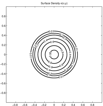
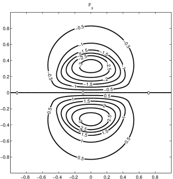
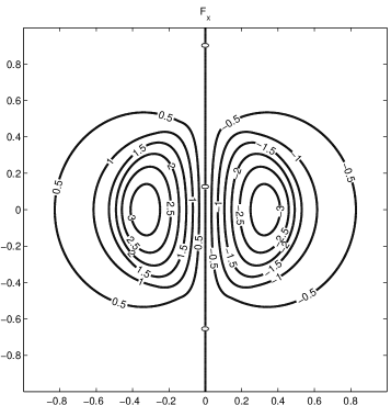
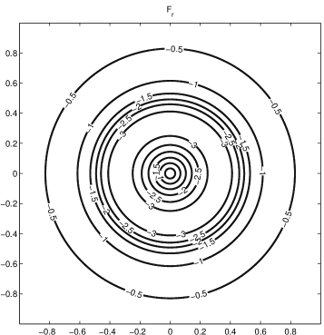
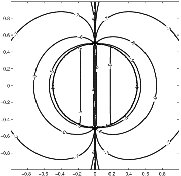
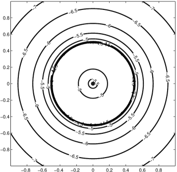
Figure 1: The numerical solutions of a $D_{2}$ disk for $N=1024$, the contour plots are surface density (upper left), the $y$-directional force (upper right), the $x$-directional force (middle left), the radial force (middle right), the difference between analytic and numerical solutions in $x$ direction (lower left), and the difference in radial direction (lower right). The values in the lower contour plots are the absolute difference in the common logarithmic scale.

We continue to use the $D_{2}$ disk as an example and a unit disk $D(0,1)=\Omega=[0,1]\times[0,2\pi]$ as the computational domain to investigate the self-gravitational force in polar coordinates. The value $\beta_{0}=0.99$ is set. We show the contour plots of the surface density, radial force, and the difference between analytic and numerical solutions for $N=512$ in Fig. 2 and the order of accuracy is only about 1 as given in Table 2. The largest errors occur in regions not only surrounding the edge of the disk, but also close to the origin. Although the surface density at the origin is smooth, the singular elliptic integral introduces significant error there. Hereafter, we concentrate on the self-gravitational forces in Cartesian coordinates.

$N$	$E^{1}_{R}$	$E^{2}_{R}$	$L^{\infty}_{R}$	$N_{k-1}/N_{k}$	$O^{1}_{R}$	$O^{2}_{R}$	$O^{\infty}_{R}$
32	1.603E-1	1.725E-1	2.725E-1
64	7.618E-2	8.289E-2	1.361E-1	32/64	1.073	1.057	1.002
128	3.646E-2	4.045E-2	6.806E-2	64/128	1.063	1.035	1.000
256	1.754E-2	2.098E-2	3.403E-2	128/256	1.056	0.947	1.000
512	8.762E-3	1.049E-2	1.701E-2	256/512	1.001	1.000	1.000

Table 2: This table demonstrates the errors and order accuracy of the proposed method for the $D_{2}$ disk for various number of zones $N=2^{k}$ from $k=5$ to $10$ on polar coordinates. It shows that the order for the $D_{2}$ disk is about 1 in each norm.

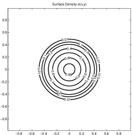
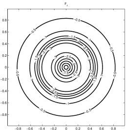
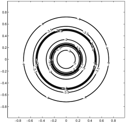
Figure 2: The numerical solutions of a $D_{2}$ disk for $N=512$ to investigate the self-gravitational force calculation in polar coordinate. From left to right, the contour plots are surface density, the radial directional force, the difference between analytic and numerical solutions, respectively. The values in the right contour plot are the absolute difference in the common logarithmic scale.

Example 2. The disk $D_{2,2}$ of two superposed $D_{2}$ has the surface density $\Sigma_{D_{2,2}}=\Sigma_{D_{2}}(R_{1};\alpha)+\Sigma_{D_{2}}(R_{2};\alpha)$, where $R_{1}=\sqrt{(x-1/4)^{2}+y^{2}}$ and $R_{2}=\sqrt{(x+1/4)^{2}+y^{2}}$. This example represents a non-symmetric distribution of the surface density of a disk. The results are shown in Table 3 and Figure 3. This result is similarly to Example 1. The factors $O^{\infty}_{x}$ of errors in Table 3 are non-monotonic as the numerical resolution, $N_{k}$, increases. This may be due to the distribution of the surface density on grid cells, the centers of which can shift with varying numerical resolution. However, the total variation and energy shows the convergence and the order of accuracy is about 1.8 and 1.9 respectively.

$N$	$E^{1}_{x}$	$E^{2}_{x}$	$E^{\infty}_{x}$	$E^{1}_{y}$	$E^{2}_{y}$	$E^{\infty}_{y}$	$E^{1}_{R}$	$E^{2}_{R}$	$L^{\infty}_{R}$
32	1.56E-2	1.29E-2	2.19E-2	2.09E-2	1.71E-2	3.57E-2	2.56E-2	1.95E-2	3.55E-2
64	4.29E-3	3.83E-3	7.75E-3	5.38E-3	4.57E-3	1.07E-2	6.89E-3	5.53E-3	1.16E-2
128	1.23E-3	1.18E-3	5.41E-3	1.50E-3	1.35E-3	5.72E-3	1.96E-3	1.64E-3	5.81E-3
256	3.17E-4	3.12E-4	1.94E-3	3.83E-4	3.54E-4	1.96E-3	5.06E-4	4.34E-4	2.01E-3
512	8.32E-5	9.00E-5	9.49E-4	9.99E-5	9.89E-5	9.53E-4	1.33E-4	1.23E-4	9.64E-4
1024	2.12E-5	2.41E-5	3.28E-4	2.54E-5	2.62E-5	3.29E-4	3.39E-5	3.29E-5	3.38E-4
$N$	$O^{1}_{x}$	$O^{2}_{x}$	$O^{\infty}_{x}$	$O^{1}_{y}$	$O^{2}_{y}$	$O^{\infty}_{y}$	$O^{1}_{R}$	$O^{2}_{R}$	$O^{\infty}_{R}$
32/64	1.86	1.75	1.50	1.96	1.87	1.74	1.89	1.82	1.62
64/128	1.80	1.71	0.52	1.85	1.79	0.90	1.81	1.75	1.00
128/256	1.96	1.91	1.48	1.97	1.93	1.55	1.95	1.92	1.53
256/512	1.93	1.79	1.03	1.94	1.84	1.04	1.93	1.81	1.06
512/1024	1.97	1.90	1.53	1.98	1.91	1.53	1.97	1.90	1.51

Table 3: This table demonstrates the errors and order of accuracy of the proposed method for the $D_{2,2}$ disk for various number of zones $N=2^{k}$ from $k=5$ to $10$. It shows that the order for the $D_{2,2}$ disk is about $1.8$ or $1.9$ order in $L^{1}$ and $L^{2}$ norm.

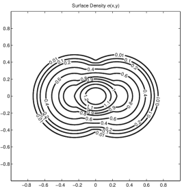
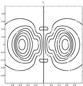
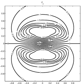
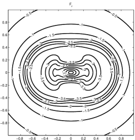
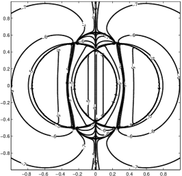
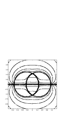
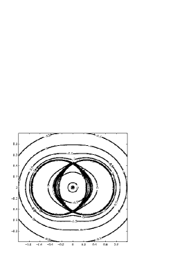
Figure 3: The numerical solutions of a $D_{2,2}$ disk for $N=1024$, The top contour plot is the surface density. The contour plots in the second row are the $x$-directional, $y$-directional, and radial forces, respectively. The corresponding errors between the numerical and analytic solutions in the third row. The values in the contour plots in the third row are the absolute errors in the common logarithmic scale.

Example 3. As another example of a non-axisymmetric potential, we consider a logarithmic spiral disk. Since an analytic pair for the surface density and potential are not known, we assume a surface density profile of the form

$$\Sigma_{LS}(r,\theta)=e^{-2r^{2}}(2+\cos(2\theta+16r)).$$

To investigate the order of accuracy, the solution at the finest mesh size is regarded as the true solution. For various coarser resolutions, the values at some specific position are taken to be the average of the four closest to the position. The results are shown for the method based on Cartesian coordinates in Table 4 and Figure 4. It can be seen that the order of accuracy is about $1.5$ for the $L^{1}$ norm and about $1$ for the $L^{2}$ norm. The $L^{\infty}$ norm is only convergent.

$N$	$E^{1}_{x}$	$E^{2}_{x}$	$E^{\infty}_{x}$	$E^{1}_{y}$	$E^{2}_{y}$	$E^{\infty}_{y}$	$E^{1}_{R}$	$E^{2}_{R}$	$L^{\infty}_{R}$
32	3.40E-1	2.97E-1	1.40E-0	3.38E-1	2.98E-1	1.39E-0	4.64E-1	3.03E-1	4.27E-1
64	1.21E-1	1.70E-1	1.83E-0	1.23E-1	1.72E-1	1.83E-0	1.36E-1	9.29E-2	2.07E-1
128	4.71E-2	9.28E-2	1.92E-0	4.83E-2	9.51E-2	1.92E-0	3.97E-2	3.93E-2	2.02E-1
256	1.87E-2	4.50E-2	1.71E-0	1.93E-2	4.68E-2	1.71E-0	1.17E-2	2.11E-2	1.75E-1
512	6.05E-3	1.67E-2	1.16E-0	6.30E-3	1.78E-2	1.16E-0	1.00E-3	9.53E-3	1.54E-1
$N$	$O^{1}_{x}$	$O^{2}_{x}$	$O^{\infty}_{x}$	$O^{1}_{y}$	$O^{2}_{y}$	$O^{\infty}_{y}$	$O^{1}_{R}$	$O^{2}_{R}$	$O^{\infty}_{R}$
32/64	1.49	0.81	-0.39	1.46	0.79	-0.40	1.77	1.70	1.05
64/128	1.36	0.87	-0.07	1.34	0.85	-0.07	1.77	1.24	0.03
128/256	1.34	1.05	0.17	1.32	1.02	0.17	1.76	0.90	0.21
256/512	1.63	1.43	0.56	1.62	1.62	0.56	1.96	1.14	0.18

Table 4: This table demonstrates the errors and order of accuracy of the proposed method for the spiral disk for various number of zones $N=2^{k}$ from $k=5$ to $9$. It shows that the order for the spiral disk is about 1.5 or 1.0 in the $L^{1}$ and $L^{2}$ norms, respectively.

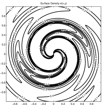
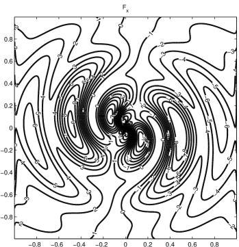
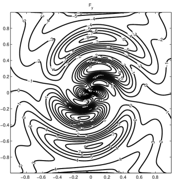
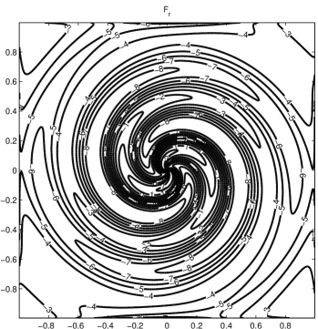
Figure 4: The numerical solutions of a logarithmic spiral disk for $N=512$ to investigate the self-gravitational force calculation. The contour plots illustrate the surface density (upper left), $x$-force (upper right), $y$-force (low left), and radial force (lower right).

5.2 A comparison study

The goal of this paper is to calculate the self-gravitational forces with as few restrictions as possible. The most straight forward approach is to solve for the potential via (1) and obtain the self-gravitational forces by taking its derivatives. If one uses the finite difference or finite element method on (1), the discretization is

$$\frac{-\Phi_{i+1,j,k}+2\Phi_{i,j,k}-\Phi_{i-1,j,k}}{(\Delta x)^{2}}+\frac{-\Phi_{i,j+1,k}+2\Phi_{i,j,k}-\Phi_{i,j-1,k}}{(\Delta y)^{2}}+\frac{-\Phi_{i,j,k+1}+2\Phi_{i,j,k}-\Phi_{i,j,k-1}}{(\Delta z)^{2}}=-f_{i,j,k}$$

where $\Phi_{i,j,k}=\Phi(x_{i},y_{j},z_{k})$ and $f_{i,j,k}=f(x_{i},y_{j},z_{k})$ based on the uniform mesh grids $(x_{i},y_{j},z_{k})$. Here, $f_{i,j,k}=0$ for $k\not=0$. For such an approach, artificial boundary conditions should be imposed and a fully 3-dimensional calculation must be undertaken. We point out that the (1) can not be reduced to the two dimensional numerical partial differential problem, i.e.,

$$\frac{-\Phi_{i+1,j,0}+2\Phi_{i,j,0}-\Phi_{i-1,j,0}}{(\Delta x)^{2}}+\frac{-\Phi_{i,j+1,0}+2\Phi_{i,j,0}-\Phi_{i,j-1,0}}{(\Delta y)^{2}}=-f_{i,j,0}.$$

Any numerical solution of the partial differential problem will involve $O(N^{3})$ unknowns. It follows that the linear complexity of such an approach, viz. multigrid method, is at least $O(N^{3})$. For an infinitesimally thin gaseous disk problem, this approach does not appear to be suitable.

Alternatively, one can solve the reduced equation given by

$$\Phi(x,y,0)=-G\int\!\!\!\int\frac{\sigma(\bar{x},\bar{y})}{\sqrt{(\bar{x}-x)^{2}+(\bar{y}-y)^{2}}}d\bar{x}d\bar{y}$$

or

$$\Phi(r,\theta,0)=-G\int\!\!\!\int\frac{\sigma(\bar{r},\bar{\theta})}{\sqrt{{\bar{r}}^{2}+r^{2}-2\bar{r}r\cos(\bar{\theta}-\theta)}}\bar{r}d\bar{r}d\bar{\theta}.$$

In this case, one can consider using bases functions on a two dimensional space as in a spectral method. Unfortunately, this approach requires a treatment for the boundary conditions. A possible way to deal with this issue is to impose periodic boundary conditions. However, it is not realistic for a gravitational force calculation because gravity is a long range force and not periodic. As an alternative, a method without the periodic assumption has been proposed for polar coordinates [3]. The approach in [3] transforms the polar coordinate $(r,\theta)$ into the coordinate $(u,\theta)$ by setting $r=e^{u}$ or $u=\ln(r)$. The potential-density pair in term of the reduced surface density and reduced potential is given in [3], and it is

$$e^{3u/2}\sigma(e^{u},\theta)=\frac{1}{4\pi^{2}}\sum_{m}\int^{\infty}_{-\infty}A_{m}(\alpha)e^{i(m\theta+\alpha u)}d\alpha$$

and

$$e^{u/2}\Phi(e^{u},\theta)=-\frac{1}{2\pi}G\sum_{m}\int^{\infty}_{-\infty}K(\alpha,m)A_{m}(\alpha)\exp[i(m\theta+\alpha u)]d\alpha,$$ (35)

where $K$ is real and positive and is defined as

$$K(\alpha,m)\equiv\frac{1}{2}\frac{\Gamma[(m+1/2+i\alpha)/2]\Gamma[(m+1/2-i\alpha)/2]}{\Gamma[(m+3/2+i\alpha)/2]\Gamma[(m+3/2-i\alpha)/2]}.$$

We regard this method as one of the spectral methods because Fourier series $e^{-im\theta}$ and Fourier integral $e^{-i\alpha u}$ are used. To apply this method to the $D_{2}$ disk using the polar coordinates, we transform the bounded unit disk $D(0,1)=[0,1]\times[0,2\pi]$ to the unbounded domain $U=(-\infty,0]\times[0,2\pi]$. In this special case, we only need to compute $m=0$ and truncate

$$A_{0}(\alpha)=\int^{0}_{-\infty}e^{3u/2}\sigma(e^{u})e^{-i\alpha u}du\approx\int^{0}_{u_{\min}}e^{3u/2}\sigma(e^{u})e^{-i\alpha u}du,$$ (36)

where the value $u_{\min}$ is to approximate $-\infty$. The truncation produces a hole in the unit disk and can introduce significant errors at the origin. Given a positive integer $N$ and base on the discretization for the radial region in the previous subsection, to calculate (36) and (35) by the trapzoidal rule. The variation of the potential with respect to radius is illustrated in Figure 5. The profile on the left panel shows that the numerical and analytic solutions for the Kalnajs’ method agree well except close to the origin for $N=1024$. The small window embedded within the panel zooms in on the residuals between numerical and analytic solution on the interval $[0,0.3]$. It is seen that the truncated portion contributes to significant errors near the origin. In contrast, the application of our proposed method to the calculation of potentials leads to the results shown in the right panel of Figure 5. Although the singular integration still remains due to the unbounded domain, our proposed method on either Cartesian and polar coordinates is preferable since a hole near the origin is not introduced.

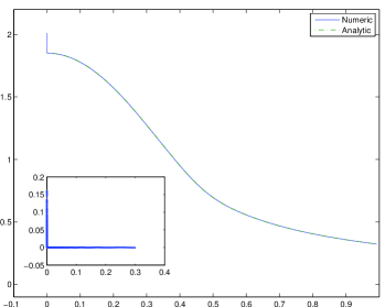
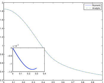
Figure 5: The variation of the potential with respect to radius using Kalnajs’ method (left) and the proposed method (right). The residuals are shown in the small window in each panel and show that the Kalnajs’ method have significant errors near the origin, which are eliminated in the proposed method.

Finally, a third approach is to directly calculate the integrals and obtain the potential. For any given mesh grid, the total amount of complexity is $O(N^{4})$ based on the number $O(N^{2})$ of mesh zones. If we restrict ourselves to a uniform grid and use the FFT technique, the complexity can be reduced from $O(N^{4})$ to $O(N^{2})$. In other words, a fast algorithm of linear complexity is obtained. It is common to start with

$$\Phi(x,y,0) = -G\int\!\!\!\int{\cal K}(\bar{x}-x,\bar{y}-y,0)\sigma(\bar{x},\bar{y})d\bar{x}d\bar{y}$$

$$= -G\sum^{N}_{i=1}\sum^{N}_{j=1}\int\!\!\!\int_{D_{i,j}}{\cal K}(\bar{x}-x,\bar{y}-y,0)\sigma(\bar{x},\bar{y})d\bar{x}d\bar{y}.$$

and to introduce a softening parameter $\epsilon$ to approximate

$$\int\!\!\!\int_{D_{i,j}}{\cal K}(\bar{x}-x,\bar{y}-y)\sigma(\bar{x},\bar{y})\approx-\frac{G}{\sqrt{\epsilon^{2}+(x_{i^{\prime}}-x_{i})^{2}+(y_{j^{\prime}}-y_{j})^{2}}}\int\!\!\!\int_{D_{i,j}}\sigma(\bar{x},\bar{y})d\bar{x}d\bar{y}.$$

Since the goal is to calculate the forces, the order of accuracy is reduced when taking the numerical differentiation on the numerical solution of potentials. For polar coordinates [1], the value of ${\cal K}$ is approximated by

$${\cal K}_{i^{\prime}-i,j^{\prime}-j}:=-\frac{G}{\sqrt{2(\cosh(u_{i^{\prime}}-u_{i})-\cos(\theta_{j^{\prime}}-\theta_{j}))}},$$

where $u_{i^{\prime}}=\ln(x_{i^{\prime}})$ and $u_{i}=\ln(x_{i})$. Note that when $(i^{\prime},j^{\prime})=(i,j)$, ${\cal K}$ is undefined. An approach to avoid the singularity problem can be found in [1]. On the other hand, the proposed method avoids the singularity problem by directly evaluating the forces, hence, raising the order of accuracy. For Cartesian coordinates, we choose the softening parameters as the mesh size $\epsilon=\Delta x$. The errors for the disks $D_{2}$ and $D_{2,2}$ are shown in Table 5 and Table 6, respectively. It reveals that the accuracy when using the softening parameter approach for the $D_{2}$ and $D_{2,2}$ disks is of first order in the $L^{1}$ and $L^{2}$ norms. For the $L^{\infty}$ norm, the order of accuracy for the $D_{2}$ disk is about $1$. For the $D_{2,2}$ disk, this method loses accuracy. In comparison with our proposed method for Example 1 and Example 2, our methods are more accurate and the order of accuracy is verified.

$N$	$E^{1}_{x}$	$E^{2}_{x}$	$L^{\infty}_{x}$	$N_{k-1}/N_{k}$	$O^{1}_{x}$	$O^{2}_{x}$	$O^{\infty}_{x}$
32	4.283E-1	5.116E-1	9.981E-1
64	2.223E-1	2.768E-1	5.415E-1	32/64	0.9461	0.8862	0.9377
128	1.133E-1	1.442E-1	2.827E-1	64/128	0.9724	0.9408	0.9377
256	5.721E-2	7.364E-2	1.440E-1	128/256	0.9858	0.9695	0.9732
512	2.874E-2	3.722E-2	7.282E-2	256/512	0.9932	0.9844	0.9837
1024	1.440E-2	1.871E-2	3.659E-2	512/1024	0.9970	0.9923	0.9929

Table 5: This table demonstrates the errors and order accuracy of the softening parameter method for the $D_{2}$ disk for various number of zones $N=2^{k}$ from $k=5$ to $10$ in Cartesian coordinates. It shows that the accuracy for the $D_{2}$ disk is about first order.

$N$	$E^{1}_{x}$	$E^{2}_{x}$	$E^{\infty}_{x}$	$E^{1}_{y}$	$E^{2}_{y}$	$E^{\infty}_{y}$	$E^{1}_{R}$	$E^{2}_{R}$	$L^{\infty}_{R}$
32	5.95E-1	5.61E-1	1.00E-0	9.13E-1	8.31E-2	1.46E-0	1.16E-0	9.32E-1	1.45E-0
64	3.10E-1	3.10E-1	5.42E-1	4.73E-1	4.49E-3	8.04E-1	5.97E-1	5.06E-1	8.04E-1
128	1.59E-1	1.69E-1	4.17E-1	2.41E-1	2.36E-3	4.22E-1	3.03E-1	2.69E-1	4.21E-1
256	8.04E-2	9.29E-2	4.17E-1	1.22E-1	1.24E-4	3.02E-1	1.53E-1	1.44E-1	4.17E-1
512	4.05E-2	5.31E-2	4.17E-1	6.10E-2	6.57E-5	3.03E-1	7.68E-2	7.85E-2	4.17E-1
1024	2.03E-2	3.19E-2	4.17E-1	3.06E-2	3.61E-5	3.03E-1	3.85E-2	4.49E-2	4.17E-1
$N$	$O^{1}_{x}$	$O^{2}_{x}$	$O^{\infty}_{x}$	$O^{1}_{y}$	$O^{2}_{y}$	$O^{\infty}_{y}$	$O^{1}_{R}$	$O^{2}_{R}$	$O^{\infty}_{R}$
32/64	0.94	0.86	0.88	0.95	0.89	0.86	0.95	0.88	0.85
64/128	0.97	0.88	0.38	0.97	0.93	0.93	0.98	0.91	0.93
128/256	0.98	0.86	0.00	0.99	0.93	0.47	0.99	0.90	0.02
256/512	0.99	0.80	0.00	0.99	0.91	0.00	0.99	0.87	0.00
512/1024	0.99	0.73	0.00	1.00	0.86	0.00	0.99	0.80	0.00

Table 6: This table demonstrates the errors and order accuracy of the softening parameter approach for the $D_{2,2}$ disk for various number of zones $N=2^{k}$ from $k=5$ to $10$. It shows that the order for the $D_{2,2}$ disk is about first order in $L^{1}$ and $L^{2}$ norm. For measurement of $L^{\infty}$ norm, this method may fail in convergence under the pointwise sense.

We implement the proposed method using MATLAB 7 software under the computer system, Intel Core 2 Duo CPU 1.8GHz with 2 GB RAM. The CPU time measurement information of the proposed method is compared with the direct method in Table 7. We list the CPU times in evaluating the kernels ${\cal K}^{\cdot,\cdot}$, the force calculations of convolutions, and the whole process. The measurement is evaluated by the mean of 40 simulations. It shows that the CPU times of both of the proposed method (P.M.) and the direct method (D.M.) are comparable.

	Kernel ${\cal K}$		Force		The whole process
$N$	P.M.	D.M.	P.M.	D.M.	P.M.	D.M.
32	9.73E-3	7.43E-3	6.10E-3	3.43E-3	1.60E-2	2.31E-2
64	3.80E-2	2.39E-2	2.08E-2	1.26E-2	5.87E-2	3.74E-2
128	1.27E-1	9.67E-2	1.06E-1	6.43E-2	2.43E-1	1.60E-1
256	5.11E-1	3.84E-1	6.48E-1	3.96E-2	1.18E+0	7.84E-1
512	2.18E+0	1.57E+0	2.75E+0	1.61E+0	4.83E+0	3.29E+0
1024	8.59E+0	6.29E+0	1.13E+1	6.49E+0	2.01E+1	1.43E+1

Table 7: This table demonstrates the CPU time measurement of the proposed method (P.M.) and direct method (D.M.) with softening parameters. The whole process consists of the generation of kernels and the forces of calculations. It shows that the CPU times of both of P.M. and D.M. are comparable.

6 Discussion and conclusion

We have presented a near second order method for calculating the self-gravitating force of an infinitesimally thin disk for Cartesian coordinates. For polar coordinates, we find that the method is near first order, $\sim 0.89$, only. To quantify the accuracy, we define

$$E_{k}=\left|\int^{\theta_{k}}_{-\theta_{k}}\ln(1-\cos(\theta))d\theta-\frac{1}{2}(\ln(1-\cos(\theta_{k}))+\ln(1-\cos(-\theta_{k}))2(\theta_{k}),\right|$$

where $\theta_{k}=1/2^{k}$. Table 8 reveals that the accuracy of the trapzoidal rule for the integration of the function $\ln(1-\cos(\theta))$ is nearly of first order. With an improvement of the singular integration of $\ln(1-\cos(\theta))$, the accuracy can be increased for the proposed method in polar coordinates.

(Term, $k$ )	2	3	4	5	6	7	8	9	10
$E_{k}$	2.86	1.73	1.07	0.55	0.34	0.20	0.11	0.06	0.03
$\log_{2}(E_{k-1}/E_{k})$		0.75	0.79	0.82	0.84	0.85	0.87	0.88	0.89

Table 8: This table demonstrates the accuracy of the trapzoidal rule for the integration of the function $\ln(1-cos(\theta))$ is near of first order $\sim 0.89$.

We note that the fast Fourier transform is only used to reduce the computational time. For the practical computation, one can extend the range of the summation in (13). By setting $\sigma_{i^{\prime},j^{\prime}}=0$ whenever either $i^{\prime}$ or $j^{\prime}$ is in the range $-N+1$ to $0$, the value of any of the $F^{x,0}_{i,j}$ is unaffected. Furthermore, we can take $\sigma_{i^{\prime},j^{\prime}}$ to be periodic since the sum (13) does not involve any values of $i^{\prime}$ and $j^{\prime}$ outside the first period. We are also free to take ${\cal K}^{x,0}_{i-i^{\prime},j-j^{\prime}}$ periodic by defining it to be the periodic function that agrees with (43) for $i-i^{\prime}$ and $j-j^{\prime}$ in the range $[-N+1,N]$ of the Green function.

An important feature of our approach is that the boundary is not assumed to be periodic. Our approach is limited to the Cartesian and polar coordinates with uniform and logarithmic grid discretization, respectively, which allows for rapid computation. That is, the restriction of a convolution of two vectors provides the rapid computation, but it is restricted to a grid discretization that is either uniform or logarithmic. If the discretization is arbitrary, then the FFT is not suitable.

We point out that our method may be useful for gravity computations on a nested grid consisting of uniform grids having different grid spacing designed to resolve a central region with a finer grid. Such an approach would be complementary to the fast algorithm for solving the Poisson equation on a nested grid presented by Matsumoto and Hanawa [5].

Appendix A: The calculation of the force in the $y$-direction in Cartesian coordinate

Let

$${\cal K}^{y,0}_{i-i^{\prime},j-j^{\prime}}=\int\!\!\!\int_{D_{i^{\prime},j^{\prime}}}\frac{(\bar{y}-y_{j})}{\left((\bar{x}-x_{i})^{2}+(\bar{y}-y_{j})^{2}\right)^{3/2}}d\bar{x}d\bar{y},$$ (37)

$${\cal K}^{y,x}_{i-i^{\prime},j-j^{\prime}}=\int\!\!\!\int_{D_{i^{\prime},j^{\prime}}}\frac{(\bar{y}-y_{j})(\bar{x}-x_{i^{\prime}})}{\left((\bar{x}-x_{i})^{2}+(\bar{y}-y_{j})^{2}\right)^{3/2}}d\bar{x}d\bar{y},$$ (38)

and

$${\cal K}^{y,y}_{i-i^{\prime},j-j^{\prime}}=\int\!\!\!\int_{D_{i^{\prime},j^{\prime}}}\frac{(\bar{y}-y_{j})(\bar{y}-y_{j^{\prime}})}{\left((\bar{x}-x_{i})^{2}+(\bar{y}-y_{j})^{2}\right)^{3/2}}d\bar{x}d\bar{y}.$$ (39)

By (6) and (9), we have

$${F}^{y}_{i,j} \approx \sum^{N}_{i^{\prime}=1}\sum^{N}_{j^{\prime}=1}\int\!\!\!\int_{D_{i^{\prime},j^{\prime}}}\frac{\partial}{\partial y}{\cal K}(\bar{x}-x_{i},\bar{y}-y_{j},0)\left(\sigma_{i^{\prime},j^{\prime}}+\delta^{x}_{i^{\prime},j^{\prime}}(\bar{x}-x_{i^{\prime}})+\delta^{y}_{i^{\prime},j^{\prime}}(\bar{y}-y_{j^{\prime}})\right)d\bar{x}d\bar{y}$$

$$:= F^{y,0}_{i,j}+F^{y,x}_{i,j}+F^{y,y}_{i,j},$$

where

$$F^{y,0}_{i,j} = \sum^{N}_{i^{\prime}=1}\sum^{N}_{j^{\prime}=1}\sigma_{i^{\prime},j^{\prime}}\int\!\!\!\int_{D_{i^{\prime},j^{\prime}}}\frac{(\bar{y}-y_{j})}{\left((\bar{x}-x_{i})^{2}+(\bar{y}-y_{j})^{2}\right)^{3/2}}d\bar{x}d\bar{y}=\sum^{N}_{i^{\prime}=1}\sum^{N}_{j^{\prime}=1}\sigma_{i^{\prime},j^{\prime}}{\cal K}^{y,0}_{i-i^{\prime},j-j^{\prime}},$$ (40)

$$F^{y,x}_{i,j} = \sum^{N}_{i^{\prime}=1}\sum^{N}_{j^{\prime}=1}\delta^{x}_{i^{\prime},j^{\prime}}\int\!\!\!\int_{D_{i^{\prime},j^{\prime}}}\frac{(\bar{y}-y_{j})(\bar{x}-x_{i^{\prime}})}{\left((\bar{x}-x_{i})^{2}+(\bar{y}-y_{j})^{2}\right)^{3/2}}d\bar{x}d\bar{y}=\sum^{N}_{i^{\prime}=1}\sum^{N}_{j^{\prime}=1}\delta^{x}_{i^{\prime},j^{\prime}}{\cal K}^{y,x}_{i-i^{\prime},j-j^{\prime}},$$ (41)

$$F^{y,y}_{i,j} = \sum^{N}_{i^{\prime}=1}\sum^{N}_{j^{\prime}=1}\delta^{y}_{i^{\prime},j^{\prime}}\int\!\!\!\int_{D_{i^{\prime},j^{\prime}}}\frac{(\bar{y}-y_{j})(\bar{y}-y_{j^{\prime}})}{\left((\bar{x}-x_{i})^{2}+(\bar{y}-y_{j})^{2}\right)^{3/2}}d\bar{x}d\bar{y}=\sum^{N}_{i^{\prime}=1}\sum^{N}_{j^{\prime}=1}\delta^{y}_{i^{\prime},j^{\prime}}{\cal K}^{y,y}_{i-i^{\prime},j-j^{\prime}}.$$ (42)

The evaluation of (37), (38) and (39) can be obtained with the help of the following simple integrals,

$$\int\!\!\!\int\frac{y}{(x^{2}+y^{2})^{3/2}}dxdy=-\ln(x+\sqrt{x^{2}+y^{2}})+C,\quad\quad\>\int\!\!\!\int\frac{xy}{(x^{2}+y^{2})^{3/2}}dxdy=-\sqrt{x^{2}+y^{2}}+C,$$

$$\int\!\!\!\int\frac{y^{2}}{(x^{2}+y^{2})^{3/2}}dxdy=x\ln(y+\sqrt{x^{2}+y^{2}})+C,\quad\int\!\!\!\int\frac{1}{(x^{2}+y^{2})^{3/2}}dxdy=-\frac{\sqrt{x^{2}+y^{2}}}{xy}+C.$$

The value ${\cal K}^{y,0}_{i-i^{\prime},j-j^{\prime}}$ is equal to

$${\cal K}^{0}_{i-i^{\prime},j-j^{\prime}}=-\ln\left((\bar{x}-x_{i})+\sqrt{(\bar{x}-x_{i})^{2}+(\bar{y}-y_{j})^{2}}\right)\left|{}^{x_{i^{\prime}+\frac{1}{2}}}_{x_{i^{\prime}-\frac{1}{2}}}\left|{}^{y_{j^{\prime}+\frac{1}{2}}}_{y_{j^{\prime}-\frac{1}{2}}}\right.\right.$$ (43)

The calculation of ${\cal K}^{y,x}_{i-i^{\prime},j-j^{\prime}}$ and ${\cal K}^{y,y}_{i-i^{\prime},j-j^{\prime}}$ are split into two parts by the identity $(\bar{y}-y_{j})(\bar{y}-y_{j^{\prime}})=(\bar{y}-y_{j})^{2}+(\bar{y}-y_{j})(y_{j}-y_{j^{\prime}})$, and $(\bar{y}-y_{j})(\bar{x}-x_{i^{\prime}})=(\bar{y}-y_{j})(\bar{x}-x_{i})+(\bar{y}-y_{j})(x_{i}-x_{i^{\prime}})$, respectively. It follows that

$${\cal K}^{y,x}_{i-i^{\prime},j-j^{\prime}} = (y_{j}-y_{j^{\prime}}){\cal K}^{y,0}_{i-i^{\prime},j-j^{\prime}}+\left((\bar{x}-x_{i})\ln(\bar{y}-y_{j}+\sqrt{(\bar{y}-y_{j})^{2}+(\bar{x}-x_{i})^{2})}\right)\left|{}^{x_{i^{\prime}+\frac{1}{2}}}_{x_{i^{\prime}-\frac{1}{2}}}\left|{}^{y_{j^{\prime}+\frac{1}{2}}}_{y_{j^{\prime}-\frac{1}{2}}}\right.\right.,$$

$${\cal K}^{y,y}_{i-i^{\prime},j-j^{\prime}} = (x_{i}-x_{i^{\prime}}){\cal K}^{y,0}_{i-i^{\prime},j-j^{\prime}}+\left(-\sqrt{(\bar{y}-y_{j})^{2}+(\bar{x}-x_{i})^{2}}\right)\left|{}^{x_{i^{\prime}+\frac{1}{2}}}_{x_{i^{\prime}-\frac{1}{2}}}\left|{}^{y_{j^{\prime}+\frac{1}{2}}}_{y_{j^{\prime}-\frac{1}{2}}}\right.\right..$$

Appendix B: Calculations of convolution of two vectors by FFT

It is known that the FFT of a vector $u_{n}$, $n=-N,\ldots,N-1$ can be rewritten as

$$\hat{u}_{k}=\sum^{N-1}_{n=-N}u_{n}e^{-j2\pi kn/2N},\mbox{ for }k=-N,\ldots,N-1,$$

and its inverse FFT is given by

$$u_{n}=\frac{1}{2N}\sum^{N-1}_{k=-N}\hat{u}_{k}e^{j2\pi kn/2N},\mbox{ for }n=-N,\ldots,N-1.$$

Let us consider two vectors $u_{n}$, $n=0,\ldots,N-1$ and $v_{n}$, $n=-N+1,\ldots,N-1$ and their inner product

$$w_{k}=\sum^{N-1}_{n=0}u_{n}v_{k-n},\mbox{ for }k=0,\ldots,N-1.$$

We set $w_{k}=0$, $k=-N,\ldots,0$ and

$$\sum^{N-1}_{k=-N}w_{k}e^{-j2\pi mk/2N} = \sum^{N-1}_{k=-N}\sum^{N-1}_{n=-N}u_{n}v_{k-n}e^{-j2\pi mk/2N}$$

$$= \sum^{N-1}_{n=-N}u_{n}e^{-j2\pi mn/2N}\sum^{N-1}_{k=-N}v_{k-n}e^{-j2\pi m(k-n)/2N}$$

$$= \sum^{N-1}_{n=-N}u_{n}e^{-j2\pi mn/2N}\sum^{N-1}_{k=-N}v_{k}e^{-j2\pi mk/2N}$$

This gives us

$$\hat{w}_{m}=\hat{u}_{m}\cdot\hat{v}_{m},\mbox{ for }m=-N,\ldots,N-1.$$

Applying the inverse FFT on the above equation, we recover the vector $w_{m}$, $m=-N,\ldots,N-1$. The vector $w_{m}$, $m=0,\ldots,N-1$ is the desired result.

References

- [1] J. Binney, S. Tremaine, Galactic Dynamics, second ed., Princeton Series in Astrophysics, 2008.
- [2] H. Johansen and P. Colella, A cartesian grid embedded boundary method for Poisson’s equation on irregular domains, J. Comput. Phys. 147 (1998) 60-85.
- [3] A. J. Kalnajs, Dynamics of flat galaxies-I, ApJ. 166 (1971) 275-293.
- [4] C.C. Lin, C. Yuan, F. H. Shu, On the spiral structure of disk galaxies. III. comparison with observations, ApJ. 155 (1969) 721-726.
- [5] T. Matsumoto, T. Hanawa, A fast algorithm for solving the Poisson equations on a nested grid, ApJ. 583 (2003) 293-307.
- [6] A.J. Roberts, Simple and fast multigrid solution of Poisson’s equation using diagonally oriented grids, ANZIAM J. 43 (2001) 1-26.
- [7] E. Schulz, Potential-Density Pairs for a Family of Finite Disks, ApJ. 693 (2009) 1310-135.
- [8] J. Shen, L.L. Wang, Some recent advances on spectral methods for unbounded domains, Comnum. Comput. Phys. 5 (2009) 195-241.
- [9] C. Yuan, D.C.C. Yen, Evolution of Self-Gravitating Gas Disks under the Influence of A Rotating Bar Potential, JKAS. 38 (2005) 197-201.
- [10] H. Zhang, C. Yuan, D.N.C. Lin, D.C.C. Yen, On the orbital evolution of a Jovian planet embedded, ApJ. 676 (2008) 639-650.
- [11] J. Zhang, Fast and high accuracy multigrid solution of the three dimensional Poisson equation, J. Comput. Phys. 143 (1998) 449-461.