On the Rate of Convergence for Critical Crossing Probabilities

Abstract

For the site percolation model on the triangular lattice and certain generalizations for which Cardy’s Formula has been established we acquire a power law estimate for the rate of convergence of the crossing probabilities to Cardy’s Formula.

^⋆Department of Mathematics, University of Toronto

^†Department of Mathematics, University of California at Los Angeles

^††Department of Mathematics, California Institute of Technology

1 Introduction

Starting with the work [14] and continuing in: [6], [17] [10], [4], [5], the validity of Cardy’s formula [7] – which describes the limit of crossing probabilities for certain percolation models – and the subsequent consequence of an SLE₆ description for the associated limiting explorer process has been well established. The purpose of this work is to provide some preliminary quantitative estimates. Similar work along these lines has already appeared in [3] (also see [12]) in the context of the so–called loop erased random walk for both the observable and the process itself. Here, our attention will be confined to the percolation observable as embodied by Cardy’s Formula for crossing probabilities.

While in the case of the loop erased random walk, estimates on the observable can be reduced to certain Green’s function estimates, in the case of percolation the observables are not so readily amenable. Instead of Green’s functions, we shall have to consider the Cauchy integral representation of the complexified crossing probability functions, as first introduced in [14]. As demonstrated in [14] (see also [2] and [10]) these functions converge to conformal maps from the domain under consideration – where the percolation process takes place – to the equilateral triangle. Thus, a combination of some analyticity property and considerations of boundary value should, in principal, yield a rate of convergence.

However, the associated procedure requires a few domain deformations, each of which must be demonstrated to be “small”, in a suitable sense. While such considerations are not important for very regular domains (which we will not quantify) in order to consider general domains, a more robust framework for quantification is called for. For this purpose, we shall introduce a procedure where all portions of the domain are explored via percolation crossing problems. This yields a multi–scale sequence of neighborhoods around each boundary point where the nature of the boundary irregularities determines the sequence of successive scales. Thus, ultimately, we are permitted to measure the distances between regions by counting the number of neighborhoods which separate them. This procedure is akin to the approach of Harris [11] in his study of the critical state at a time when detailed information about the nature of the state was unavailable.

Ultimately we establish a power law estimate (in mesh size) for the rate of convergence in any domain with boundary dimension less than two. (For a precise statement see the Main Theorem below.) As may or may not be clear to the reader at this point the hard quantifications must be done via percolation estimates – as is perhaps not surprising since we cannot easily utilize continuum estimates before having reached the continuum in the first place. The plausibility of a power law estimate then follows from the fact that most a priori percolation estimates are of this form.

Finally, we should mention that this problem is also treated in the posting [15], which appeared at approximately the same time as (the preliminary version of) the present work. The estimates in [15] are more quantitative, however, the class of domains treated therein are restricted. In the present work we make no efforts towards precise quantification, but we shall treat the problem for essentially arbitrary domains. It is remarked that convergence to Cardy’s Formula in a general class of domains is, most likely, an essential ingredient for acquiring a rate of convergence to SLE₆ for the percolation interfaces.

2 Preliminaries

2.1 The Models Under Consideration

We will be considering critical percolation models in the plane. However in contrast to the generality professed in [4], [5] – where, essentially, “all” that was required was a proof of Cardy’s formula, here the mechanism of how Cardy’s formula is established will come into play. Thus, we must restrict attention to the triangular site percolation problem considered in [14] and the generalization provided in [10]. These models can all be expressed in terms of random colorings (and sometimes double colorings) of hexagons. As is traditional, the competing colors are designated by blue and yellow. We remind the reader that criticality implies that there are scale independent bounds in $(0,1)$ for crossing probabilities – in either color – between non–adjacent sides of regular polygons. In this work, for the most part, we will utilize crossings in rectangles with particular aspect ratios.

2.2 The Observable

Consider a fixed domain $\Omega\subset\mathbb{C}$ that is a conformal rectangle with marked points (or prime ends) $A$, $B$, $C$ and $D$ which, as written, are in cyclic order. We let $\Omega_{n}$ denote the lattice approximation at scale $\varepsilon=n^{-1}$ to the domain $\Omega$. The details of the construction of $\Omega_{n}$ – especially concerning boundary values and explorer processes – are somewhat tedious and have been described e.g., in [5] §3 $\&$ §4 and [4] §4.2. For present purposes, it is sufficient to know that $\Omega_{n}$ consists of the maximal union of lattice hexagons – of radius $1/n$ – whose closures lie entirely inside $\Omega$; we sometimes refer to this as the canonical approximation. (We shall also have occasions later to use other discrete interior approximating domains which are a subset of $\Omega_{n}$.) Moreover, boundary arcs can be appropriately colored and lattice points $A_{n}$ – $D_{n}$ can be selected. We consider percolation problems in $\Omega_{n}$.

The pertinent object to consider is a crossing probability: performing percolation on $\Omega_{n}$, we ask for the crossing probability – say in yellow – from $(A_{n},B_{n})$ to $(C_{n},D_{n})$. Here and throughout this work, a colored crossing necessarily implies the existence of a self–avoiding, connected path of the designated color with endpoints in the specified sets and/or that satisfies specific separation criteria. Below we list various facts, definitions and notations related to the observable that will be used throughout this work. In some of what follows, we temporarily neglect the marked point $A_{n}$ and regard $\Omega_{n}$ with the three remaining marked points as a conformal triangle.

• Let us recall the functions introduced in [14], here denoted by $S_{B},S_{C},S_{D}$ where e.g., $S_{D}(z)$ with $z\in\Omega_{n}$ a lattice point, is the probability of a yellow crossing from $(C_{n},D_{n})$ to $(D_{n},B_{n})$ separating $z$ from $(B_{n},C_{n})$. Note that it is implicitly understood that the $S_{B},S_{C},S_{D}$–functions are defined on the discrete level; to avoid clutter, we suppress the $n$ index for these functions. Moreover, we will denote the underlying events associated to these functions by $\mathbb{S}_{B},\mathbb{S}_{C},\mathbb{S}_{D}$, respectively.

• It is the case that the functions $S_{B},S_{C},S_{D}$ are invariant under exchange of color (see [14] and [10]). While it is not essential to the arguments in this work, we sometimes may take liberties regarding whether we are considering a yellow or blue version of these functions.

• It is also easy to see that e.g., $S_{B}$ has boundary value 0 on $(C_{n},D_{n})$ and 1 at the point $B_{n}$. Moreover, the complexified function $S_{n}=S_{B}+\tau S_{C}+\tau^{2}S_{D}$, with $\tau=e^{2\pi i/3}$, converges to the conformal map to the equilateral triangle with vertices at $1,\tau,\tau^{2}$, which we denote by $\mathbb{T}$. (See [14], [2], [5].)

• For finite $n$, we shall refer to the object $S_{n}(z)$ as the Carleson–Cardy–Smirnov function and sometimes abbreviated CCS–function.

• We will use $H_{n}:\Omega_{n}\rightarrow\mathbb{T}$ to denote the unique conformal map which sends $(B_{n},C_{n},D_{n})$ to $(1,\tau,\tau^{2})$. Similarly, $H:\Omega\rightarrow\mathbb{T}$ is the corresponding conformal map of the continuum domain.

• With $A_{n}$ reinstated, we will denote by $\mathscr{C}_{n}$ the crossing probability of the conformal rectangle $\Omega_{n}$ and $\mathscr{C}_{\infty}$ its limit in the domain $\Omega$; i.e., Cardy’s Formula in the limiting domain.

• Since $S_{C}(A_{n})\equiv 0$,

  $$S_{n}(A_{n})=S_{B}(A_{n})+\tau^{2}S_{D}(A_{n})=[S_{B}(A_{n})-\frac{1}{2}S_{D}(A_{n})]-i\frac{\sqrt{3}}{2}S_{D}(A_{n}).$$

  Now we recall (or observe) that $\mathscr{C}_{n}$ can be realized as $S_{D}(A_{n})$ and so from the previous display, $\mathscr{C}_{n}=-\frac{2}{\sqrt{3}}\cdot\mbox{Im}[S_{n}(A_{n})]$. Since it is already known that $S_{n}$ converges to $H$ (see [14], [2], [5]) it is also the case that $\mathscr{C}_{\infty}=-\frac{2}{\sqrt{3}}\cdot\mbox{Im}[H(A)]$. Therefore to establish a rate of convergence of $\mathscr{C}_{n}$ to $\mathscr{C}_{\infty}$, it is sufficient to show that there is some $\psi>0$ such that

  $$|S_{n}(A_{n})-H(A)|\leq C_{\psi}\cdot n^{-\psi},$$

  for some $\psi>0$ and $C_{\psi}<\infty$ which may depend on the domain $\Omega$.

• The functions $S_{n}$ are not discrete analytic but the associated contour integrals vanish with lattice spacing (see [14], [2] and [10].) In particular, this is exhibited by the fact that the contour integral around some closed discrete contour $\Gamma_{n}$ behaves like the length of $\Gamma_{n}$ times $n$ to some negative power. Also, the functions $S_{n}$ are Hölder continuous with estimates which are uniform for large $n$. For details we refer the reader to Definition 4.1.

Our goal in this work is to acquire the following theorem on the rate of convergence of the finite volume crossing probability, $\mathscr{C}_{n}$, to its limiting value:

Main Theorem.

Let $\Omega$ be a domain and $\Omega_{n}$ its canonical discretization. Consider the site percolation model or the models introduced in [10] on the domain $\Omega_{n}$. In the case of the latter we also impose the assumption that the boundary Minkowski dimension is less than 2 (in the former, this is not necessary). Let $\mathscr{C}_{n}$ be described as before. Then there exists some $\psi(\Omega)>0$ (which may depend on the domain $\Omega$) such that $\mathscr{C}_{n}$ converges to its limit with the estimate

$$|\mathscr{C}_{n}-\mathscr{C}_{\infty}|\lesssim n^{-\psi},$$

provided $n\geq n_{0}(\Omega)$ is sufficiently large and the symbol $\lesssim$ is described with precision in Notation 2.1 below.

Notation 2.1

In the above and throughout this work, we will be describing asymptotic behaviors of various quantities as a function of small or large parameters (usually $n$ in one form or another). The relation $X\lesssim Y$ relating two functions $X$ and $Y$ of large or small parameters (below denoted by $M$ and $m$, respectively) means that there exists a constant $c\in(0,\infty)$ independent of $m$ and $M$ such that for all $M$ sufficiently large and/or $m$ sufficiently small $X(m,M)\leq c\cdot Y(m,M)$.

Remark 2.2.

The restrictions on the boundary Minkowski dimension for the models in [10] is not explicitly important in this work and will only be implicitly assumed as it was needed in order to establish convergence to Cardy’s Formula.

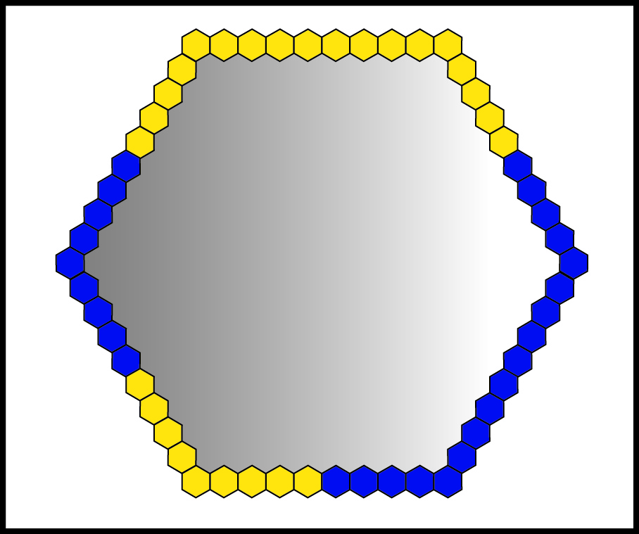
Figure 1: In certain conformal rectangles, the crossing probabilities at the discrete level will be identically $\frac{1}{2}$ independent of scale.

Remark 2.3.

It would seem that complementary lower bounds of the sort presented in the Main Theorem are actually not possible. For example, in the triangular site model, the crossing probabilities for particular shapes are identically $\tfrac{1}{2}$ independently of $n$, as is demonstrated in Figure 1.

We end this preliminary section with some notations and conventions: (i) the notation $\mbox{dist}(\cdot,\cdot)$ denotes the usual Euclidean distance while the notation $d_{\rm sup}(\cdot,\cdot)$ denotes the sup–norm distance between curves; (ii) we will make use of both macroscopic and microscopic units, with the former corresponding to an $\varepsilon\rightarrow 0$ approximation to shapes of fixed scale and the latter corresponding to $n\rightarrow\infty$, wherein distances are measured relative to the size of a hexagon. So, even though analytical quantities are naturally expressed in macroscopic units, it is at times convenient to use microscopic units when performing percolation constructions; (iii) we will use $a_{1},a_{2},\dots$ to number the powers of $n$ appearing in the statements of lemmas, theorems, etc. Thus, throughout, $n=\varepsilon^{-1}$. Constants used in the course of a proof are considered temporary and duly forgotten after the Halmos box.

3 Proof of the Main Theorem

Our strategy for the proof of the Main Theorem is as follows: recall that $H_{n}$ is the conformal map from $\Omega_{n}$ to $\mathbb{T}$ (the “standard” equilateral triangle) so that $B_{n},C_{n},D_{n}$ map to the three corresponding vertices, where it is reiterated that $\mathscr{C}_{n}$ corresponds to a boundary value of $S_{n}$. Thus it is enough to uniformly estimate the difference between $S_{n}$ and $H_{n}$ and then the difference between $H_{n}$ and $H$.

Foremost, the discrete domain may itself be a bit too rough so we will actually be working with an approximation to $\Omega_{n}$ which will be denoted by $\Omega_{n}^{\square}$ (see Proposition 3.2). Now, on $\Omega_{n}^{\square}$, we have the function $S_{n}^{\square}$ associated with the corresponding percolation problem on this domain and, similarly, the conformal map $H_{n}^{\square}:\Omega_{n}^{\square}\to\mathbb{T}$. Via careful consideration of Euclidean distances and distortion under the conformal map, we will be able to show that both $|S_{n}(A_{n})-S_{n}^{\square}(A_{n}^{\square})|$ (for an appropriately chosen $A_{n}^{\square}\in\partial\Omega_{n}^{\square}$) and $|H(A)-H_{n}^{\square}(A_{n}^{\square})|$ are suitably small (see Theorem 3.3). Thus we are reduced to proving a power law estimate for the domain $\Omega_{n}^{\square}$.

Towards this goal, we introduce the Cauchy–integral extension of $S_{n}^{\square}$, which we denote by $F_{n}^{\square}$, so that

$$F_{n}^{\square}(z):=\frac{1}{2\pi i}\oint_{\partial\Omega_{n}^{\square}}\frac{S_{n}^{\square}(\zeta)}{\zeta-z}~{}d\zeta.$$

Now by using the Hölder continuity properties and the approximate discrete analyticity properties of the $S_{n}$’s, we can show that, barring the immediate vicinity of the boundary, the difference between $F_{n}^{\square}$ and $S_{n}^{\square}$ is power law small (see Lemma 3.5). It follows then that in an even smaller domain, $\Omega_{n}$, which can be realized as the inverse image of a uniformly shrunken version of $\mathbb{T}$, the function $F_{n}^{\square}$ is in fact conformal and thus it is uniformly close to $H_{n}$, which is the conformal map from $\Omega_{n}$ to $\mathbb{T}$ (see Lemma 3.9).

Now for $z\in\Omega_{n}^{\square}$ the dichotomy we have introduced is not atypical: on the one hand, $F_{n}^{\square}(z)$ is manifestly analytic but does not necessarily embody the function $S_{n}^{\square}$ of current interest. On the other hand, $S_{n}^{\square}(z)$ has the desired boundary values – at least on $\partial\Omega_{n}^{\square}$ – but is, ostensibly, lacking in analyticity properties. Already the approximate discrete analyticity properties permit us to compare $F_{n}^{\square}$ to $S_{n}^{\square}$ in $\Omega_{n}$. In order to return to the domain $\Omega_{n}^{\square}$, we require some control on the “distance” between $\Omega_{n}$ and $\Omega_{n}^{\square}$ (not to mention a suitable choice of some point $A_{n}\in\partial\Omega_{n}$ as an approximation to $A$). It is indeed the case that if $\Omega_{n}$ is close to $\Omega_{n}^{\square}$ in the Hausdorff distance, then the proof can be quickly completed by using distortion estimates and/or Hölder continuity of the $S$ function. However, such information translates into an estimate on the continuity properties of the inverse of $F_{n}^{\square}$, which is not a priori accessible (and, strictly speaking, not always true).

Further thought reveals that we in fact require the domain $\Omega_{n}$ to be close to $\Omega_{n}^{\square}$ in both the conformal sense and in the sense of “percolation” – which can be understood as being measured via local crossing probabilities. (In principle, given sufficiently strong control on boundary distortion of the relevant conformal maps, these notions should be directly equivalent; however, we do not explicitly address this question here, as this would entail overly detailed consideration of domain regularity.)

While with a deliberate choice of a point on the boundary corresponding to $A$ we may be able to ensure that either one or the other of the two criteria can be satisfied, it is not readily demonstrable that both can be simultaneously satisfied without some additional detailed considerations; it is for this reason that we will introduce and utilize the notion of Harris systems (see Theorem 3.10) in order to quantify the distances between $\Omega_{n}$ and $\Omega_{n}^{\square}$.

The Harris systems are collections of concentric topological rectangles (portions of annuli) of various scales centered on points of $\partial\Omega_{n}^{\square}$ and heading towards some “central region” of $\Omega_{n}^{\square}$; they are constructed so that uniform estimates are available for both the traversing of each annular portion and the existence of an obstructing “circuit” (in dual colors). This leads to a natural choice of $A_{n}$: it is a point on $\partial\Omega_{n}$ which is in the Harris system of $A_{n}^{\square}$ (i.e., a point in one of the “rings”). Consequently, the distance between $A_{n}^{\square}$ and $A_{n}$ – and other such pairs as well – can be measured vis a counting of Harris segments (see Lemma 3.12).

Specifically, we will make use of another auxiliary point, $A_{n}^{\diamondsuit}$, which is also in the Harris system centered at $A_{n}^{\square}$, chosen so that it is inside the domain $\Omega_{n}$. The task of providing an estimate for $|S_{n}^{\square}(A_{n}^{\diamondsuit})-S_{n}^{\square}(A_{n}^{\square})|$ (and thus also $|F_{n}^{\square}(A_{n}^{\diamondsuit})-S_{n}^{\square}(A_{n}^{\square})|$) is immediately accomplished by the existence of suitably many Harris segments surrounding both $A_{n}^{\square}$ and $A_{n}^{\diamondsuit}$ (see Proposition 3.15). Also, considering $n$ to be fixed, the domain $\Omega_{n}^{\square}$ can be approximated at scales $N^{-1}\ll n^{-1}$ and the estimates derived from the Harris systems remain uniform in $N$ as $N$ tends to infinity and thus also immediately imply an estimate for $|H_{n}^{\square}(A_{n}^{\square})-H_{n}^{\square}(A_{n}^{\diamondsuit})|$ (see Proposition 3.14).

At this point what remains to be established is an estimate relating the conformal map $H_{n}$, which is defined by percolation at scale $n$ via $F_{n}^{\square}$, and $H_{n}^{\square}$, the “original” conformal map. It is here that we shall invoke a Marchenko theorem for the triangle $\mathbb{T}$ (see Lemma 3.16): indeed, again considering $\Omega_{n}^{\square}$ to be a fixed domain and performing percolation at scales $N^{-1}\ll n^{-1}$, we have by convergence to Cardy’s Formula that $S_{n,N}^{\square}(s)\rightarrow H_{n}^{\square}(s)$ as $N\rightarrow\infty$, for all $s\in\partial\Omega_{n}$. The inherent scale invariance of the Harris systems permits us to establish that in fact $S_{n,N}^{\square}(s)$ is close to $\partial\mathbb{T}$, uniformly in $N$ (see Lemma 3.18) and thus, $H_{n}^{\square}(\partial\Omega_{n})$ is close to $\partial\mathbb{T}$ (in fact in the supremum norm). Armed with this input, the relevant Marchenko theorem applied at the point $A_{n}^{\diamondsuit}$ immediately gives that $H_{n}^{\square}(A_{n}^{\diamondsuit})-H_{n}(A_{n}^{\diamondsuit})$ is suitably small.

The technical components relating to the Cauchy–integral estimate and the construction of the Harris systems are relegated to Section 4 and Section 5, respectively. As for the rest, we will divide the proof of the main theorem into three subsections, corresponding to:

• the regularization of the boundary (introduction of $\Omega_{n}^{\square}$) and showing that crossing probabilities are close for the domains $\Omega_{n}^{\square},\Omega_{n}~{}\&~{}\Omega$;

• the construction of the Cauchy–integral $F_{n}^{\square}$ and of the domain $\Omega_{n}$;

• the establishment of the remaining estimates needed to show that the domains $\Omega_{n}$ and $\Omega_{n}^{\square}$ are suitably close, by using the Harris systems of neighborhoods.

3.1 Regularization of Boundary Length

We now introduce the domain $\Omega_{n}^{\square}\subseteq\Omega_{n}$. The primary purpose of this domain is to reduce the boundary length of the domain that need be considered; in particular, this will be pivotal when estimating the discrete analyticity properties of $S_{n}^{\square}$ in the next section.

Definition 3.1.

Let $1>a_{1}>0$ and consider a square grid whose elements are squares of (approximately) microscopic size $n^{a_{1}}$ and let $\Omega^{\square}_{n}$ denote the union of all (hexagons within the) squares of this grid that are entirely within the original domain $\Omega$.

We have:

Proposition 3.2

Let $\Omega\subseteq\mathbb{C}$ be a domain with boundary Minkowski dimension at most $1+\alpha^{\prime}$ with $\alpha^{\prime}\in[0,1]$, which we write as $M(\partial\Omega)<1+\alpha$ for any $\alpha>\alpha^{\prime}$. Then the domain $\Omega_{n}^{\square}$ satisfies $\Omega_{n}^{\square}\subseteq\Omega_{n}$ and

$$|\partial\Omega_{n}^{\square}|\lesssim n^{\alpha(1-a_{1})}.$$

Proof.

Since $M(\partial\Omega)<1+\alpha$ we have (for all $n$ sufficiently large) that the number of boxes required to cover $\partial\Omega$ is essentially bounded from above by $(n^{1-a_{1}})^{1+\alpha}$ which is then multiplied by $\frac{1}{n^{(1-a_{1})}}$, the size of the box (in macroscopic units). The fact that $\Omega_{n}^{\square}\subseteq\Omega_{n}$ is self–evident. ∎

Next we will choose $A_{n}^{\square},B_{n}^{\square},C_{n}^{\square},D_{n}^{\square}\in\partial\Omega_{n}^{\square}$ by some procedure to be outlined below and denote by $S_{n}^{\square}$ the corresponding CCS–function. Particularly, this can be done so that the crossing probabilities do not change much:

Theorem 3.3

Let $\Omega_{n}^{\square}\subseteq\Omega_{n}$ with marked boundary points $(A_{n},\dots,D_{n})$ be as described, so particularly $\partial\Omega_{n}^{\square}$ is of distance at most $n^{1-a_{1}}$ from $\partial\Omega_{n}$. Then there is an $A_{n}^{\square}$ as well as $B_{n}^{\square}$, $C_{n}^{\square}$ and $D_{n}^{\square}$ such that the corresponding $S_{n}^{\square}$ satisfies, for some $a_{2}>0$ and for all $n$ sufficiently large,

$$|S_{n}(A_{n})-S_{n}^{\square}(A_{n}^{\square})|\lesssim n^{-a_{2}}$$

and, moreover,

$$|H(A)-H_{n}^{\square}(A_{n}^{\square})|\lesssim n^{-a_{2}}.$$

Remark 3.4.

In the case that the separation between $A_{n}$ and $\partial\Omega_{n}$ is the order of $n^{a_{1}}$ – as is usually imagined – facets of Theorem 3.3 are essentially trivial. However, the reader is reminded that $A_{n}$ could be deep inside a “fjord” and well separated from $\partial\Omega_{n}^{\square}$. In this language, the forthcoming arguments will demonstrate that, notwithstanding, an $A_{n}^{\square}$ may be chosen near the mouth of the fjord for which the above estimates hold.

Proof of Theorem 3.3. For $\eta>0$ and a subset $K\subset\overline{\Omega}$ we will denote by $N_{\eta}(K)$ the $\eta$–neighborhood of $K$ intersected with $\Omega$. Now let us first choose $\eta$ sufficiently small so that

$$\left[[B,C,D]\cup N_{4\eta}(B)\cup N_{4\eta}(D)\cup N_{4\eta}(C)\right]\cap N_{4\eta}(A)=\emptyset,$$

where $[B,C,D]$ denotes the closed boundary segment containing the prime ends $B,C,D$.

Next we assume that $n>n_{\circ}$ where $n_{\circ}$ is large enough so that for all $n>n_{\circ}$, $A_{n}\in N_{\eta}(A)$ , …, $D_{n}\in N_{\eta}(D)$. Moreover, $\Omega_{n}^{\square}\cap N_{\eta}(A)\neq\emptyset$ and similarly for $\Omega_{n}^{\square}\cap N_{\eta}(B),\dots,\Omega_{n}^{\square}\cap N_{\eta}(D)$. Then, since

$$0<\text{dist}(([A,B]\setminus N_{\eta}(A)),([D,A]\setminus N_{\eta}(A)))$$

it is assumed that for $n>n_{\circ}$, the above is very large compared with $n^{-(1-a_{1})}$ and similarly for the other three marked points. Finally, consider the uniformization map $\varphi:\mathbb{D}\rightarrow\Omega$. Then taking $n_{\circ}$ larger if necessary, we assert that for all $n>n_{\circ}$, the distance (in the unit disc) between $\varphi^{-1}(N_{\eta}(A))$ and $[\varphi^{-1}(N_{4\eta}(A))]^{\text{c}}$ satisfies

$$\text{dist}[\varphi^{-1}(N_{\eta}(A)),[\varphi^{-1}(N_{4\eta}(A))]^{\text{c}}]\gg n^{-\frac{1}{2}}.$$ (3.1)

We first state:

Claim. For $n>n_{\circ}$,

$$\mbox{dist}(N_{\eta}(A),[B_{n},C_{n},D_{n}])>0.$$

Proof of Claim. We note that the pre–image of $\partial\Omega_{n}$ under uniformization has the following property: for $n$ sufficiently large as specified above, consider the pre–image of the boundary element $\varphi^{-1}([A_{n},B_{n}])$. Then starting at $\varphi^{-1}(A_{n})$, once the segment enters $\varphi^{-1}(N_{\eta}(B_{n}))$, it must hit $\varphi^{-1}(B_{n})$ before exiting $\varphi^{-1}(N_{4\eta}(B_{n}))$.

Indeed, if this were not true, then necessarily there would be three or more crossings of the “annular region” $\varphi^{-1}(N_{4\eta}(B_{n}))\setminus\varphi^{-1}(N_{\eta}(B_{n}))$. It is noted that all such crossings – indeed all of $\varphi^{-1}(\Omega_{n})$ – lies within a distance of the order $n^{-1/2}$ of $\partial\mathbb{D}$. This follows by standard distortion estimates (see e.g., [13], Corollary 3.19 together with Theorem 3.21) and the definition of canonical approximation: each point on $\partial\Omega_{n}$ is within distance $1/n$ of some point on $\partial\Omega$. It is further noted, by the final stipulation concerning $n_{\circ}$, that the separation scale of the above mentioned “annular region” is large compared with the distance $n^{-1/2}$.

Envisioning $\partial\Omega$ to be the “bottom”, consider now a point on the “topmost” of these crossings which is well away – compared with $n^{-1/2}$ – from the lateral boundaries of the annular region and also the pre–image of its associated hexagon. Since this point is the pre–image of one on $\partial\Omega_{n}$, the hexagon in question must intersect $\partial\Omega$ and therefore its pre–image must intersect $\partial\mathbb{D}$. However, in order to intersect $\partial\mathbb{D}$, the pre–image of the hexagon in question must intersect all the lower crossings, since our distortion estimate does not permit this pre–image to leave (a lower portion of) the annular region. This necessarily implies it passes through the interior of $\Omega_{n}$, which is impossible for a boundary hexagon.

The same argument also shows that once $\varphi^{-1}(\partial\Omega_{n})$ exits $\varphi^{-1}(N_{4\eta}(B_{n}))$, it cannot re–enter $\varphi^{-1}(N_{\eta}(B_{n}))$ and so must be headed towards $\varphi^{-1}(C_{n})$ and certainly cannot enter $\varphi^{-1}(N_{\eta}(A))$ since

$$\mbox{dist}(\varphi^{-1}(N_{\eta}(A)),\varphi^{-1}([B,C,D]\cup[N_{4\eta}(B)\cup N_{4\eta}(D)\cup N_{4\eta}(C)]))\gg n^{-1/2}$$

by assumption (by the choice of $\eta$, it is the case that $[B,C,D]\cup[N_{4\eta}(B)\cup N_{4\eta}(D)\cup N_{4\eta}(C)]\subseteq[N_{4\eta}(A)]^{c}$ from which the previous display follows from Equation (3.1)).

Altogether we then have that $\mbox{dist}(\varphi^{-1}(N_{\eta}(A)),\varphi^{-1}([B_{n},C_{n},D_{n}]))>0$, and so the claim follows after applying $\varphi$. ∎

The above claim in fact implies that there exist points $A_{n}^{p}\in[A_{n},B_{n}]$ and $A_{n}^{g}\in[A_{n},D_{n}]$ such that

$$\mbox{dist}(A_{n}^{p},A_{n}^{g})<\frac{1}{n^{1-a_{1}}}$$

and

$$\mbox{dist}(A_{n}^{p},\partial\Omega_{n}^{\square}),~{}\mbox{dist}(A_{n}^{g},\partial\Omega_{n}^{\square})<\frac{1}{n^{1-a_{1}}}.$$

Indeed, consider squares of side length $n^{a_{1}}$ intersecting $\partial\Omega_{n}$ which share an edge with $\partial\Omega_{n}^{\square}$ and have non–trivial intersection with $N_{\eta}(A)$, then since $\partial\Omega_{n}$ passes through such boxes, we can unambiguously label them as either an $[A_{n},B_{n}]$, an $[A_{n},D_{n}]$ box, or both, and by the claim there are no other possibilities. Therefore, a pair of such boxes of differing types must be neighbors or there is at least one single box of both types, so we indeed have points $A_{n}^{p},A_{n}^{g}$ as claimed. Finally, by the stipulation

$$\frac{1}{n^{1-a_{1}}}\ll\text{dist}(([A,B]\setminus N_{\eta}(A)),([D,A]\setminus N_{\eta}(A)))$$

it is clear that these points must lie in $N_{\eta}(A)$.

Thus we choose $A_{n}^{\square}\in\partial\Omega_{n}^{\square}$ to be any point near the $(A_{n}^{p},A_{n}^{g})$ juncture (e.g., the nearest point). Now consider the scale $n^{a_{3}}$ with $1>a_{3}>a_{1}$. We may surround the points $A_{n}^{p},A_{n}^{g}$ and $A_{n}^{\square}$ with the order of $\log_{2}n^{a_{3}-a_{1}}$ disjoint concentric annuli. These annuli have the property that the fragment consisting of its intersection with $\Omega_{n}$ forms a conduit between some portion of the $[A_{n},D_{n}]$ boundary (which need not be connected) and a similar portion of the $[A_{n},B_{n}]$ boundary. Moreover, any circuit in the annulus necessarily provides a path which connects these two portions. Thus the probability of a blue connected path between $[A_{n},D_{n}]$ and $[A_{n},B_{n}]$ within any particular annulus fragment is no less than the probability of a blue circuit in the corresponding full annulus, which is uniformly positive. So letting $\mathcal{A}$ denote the event that in at least one of these fragments the desired blue connection occurs, we have

$$\mathbb{P}(\mathcal{A})\geq 1-n^{-a_{4}}$$ (3.2)

for some $a_{4}>0$. Similar constructions may be enacted about the $B_{n},B_{n}^{\square};\dots;D_{n},D_{n}^{\square}$ pairs leading, ultimately, to the events $\mathcal{B},\dots,\mathcal{D}$ (which are analogous to $\mathcal{A}$) with estimates on their probabilities as in Eq.(3.2). For future reference, we denote by $\mathcal{E}$ the event $\mathcal{A}\cap\dots\cap\mathcal{D}$ and so $\mathbb{P}(\mathcal{E})\gtrsim 1-n^{a_{4}}$ (by the FKG inequality).

We are now in a position to verify that $|S_{n}(A_{n})-S_{n}^{\square}(A_{n}^{\square})|$ obeys the stated power law estimate. Indeed, the $C$–component of both functions vanish identically while the differences between the other two components amount to comparisons of crossing probabilities on the “topological” rectangles $[A_{n},B_{n},C_{n},D_{n}]$ verses $[A_{n}^{\square},B_{n}^{\square},C_{n}^{\square},D_{n}^{\square}]$. There are two crossing events contributing to the (complex) function $S_{n}(A_{n})$ (and similarly for $S_{n}^{\square}(A_{n}^{\square})$) but since the arguments are identical, it is sufficient to treat one such crossing event. Thus we denote by $\mathbb{K}_{n}$ the event of a crossing in $\Omega_{n}$ by a blue path between the $[A_{n},D_{n}]$ and $[B_{n},C_{n}]$ boundaries (the event contributing to $S_{B}(A_{n})$) and similarly for the event $\mathbb{K}_{n}^{\square}$ for a blue path in $\Omega_{n}^{\square}$. It is sufficient to show that $|\mathbb{P}(\mathbb{K}_{n}^{\square})-\mathbb{P}(\mathbb{K}_{n})|$ has an estimate of the stated form.

The greater portion of the following is rather standard in the context of 2D percolation theory so we shall be succinct. The idea is to first “seal” together e.g., $A_{n}$ and $A_{n}^{\square}$ (and similarly for $B,C,D$) by circuits and then perform a continuation of crossings argument.

Without loss of generality we may assume that $S_{B}^{\square}(A_{n}^{\square})>S_{B}(A_{n})$ since otherwise the $S_{D}$ functions would satisfy this inequality and we may work with $S_{D}$ instead. For ease of exposition, let us envision $[A_{n},B_{n}]$ and $[A_{n}^{\square},B_{n}^{\square}]$ as the “bottom” boundaries and the $D,C$ pairs as being on the “top”.

Let $\Gamma$ denote a crossing between $[A_{n}^{\square},D_{n}^{\square}]$ and $[B_{n}^{\square},C_{n}^{\square}]$ within $\Omega_{n}^{\square}$ and let $\Gamma_{\mathbb{K}_{n}^{\square}}\in\mathbb{K}_{n}^{\square}$ denote the event that $\Gamma$ is the “lowest” (meaning $[A_{n}^{\square},B_{n}^{\square}]$–most) crossing. These events form a disjoint partition so that $\mathbb{P}(\mathbb{K}_{n}^{\square})=\sum_{\Gamma}~{}\mathbb{P}(\mathbb{K}_{n}^{\square}\mid\Gamma_{\mathbb{K}_{n}^{\square}})\cdot\mathbb{P}(\Gamma_{\mathbb{K}_{n}^{\square}})$. From previous discussions concerning $A_{n}^{p},A_{n}^{g}$, we have that $\mathbb{P}(\mathcal{E})\geq 1-n^{-a_{4}}$, which we remind the reader, means that with the stated probability, these crossings do not go into any “corners” and hence there is “ample space” to construct a continuation.

So let $a_{5}>a_{1}$ denote another constant which is less than unity (recall that in microscopic units, $\mbox{dist}(\partial\Omega_{n}^{\square},\partial\Omega_{n})\leq n^{a_{1}}$). Then, to within tolerable error estimate (by the Russo–Seymour–Welsh estimates) it is sufficient to consider only the crossings $\Gamma$ with right endpoint a distance in excess of $n^{a_{5}}$ away from $C_{n}^{\square}$ and with left endpoint similarly separated from $D_{n}^{\square}$.

Let $\Gamma_{D}$ and $\Gamma_{C}$ denote these left and right endpoints of $\Gamma$, respectively. Consider a sequence of intercalated annuli starting at the scale $n^{a_{1}}$ – or, if necessary, in slight excess – and ending at scale $n^{a_{5}}$ (where ostensibly they might run aground at $C_{n}^{\square}$) around $\Gamma_{C}$. A similar sequence should be considered on the left. Focusing on the right, it is clear that each such annulus provides a conduit between $\Gamma$ and $\partial\Omega_{n}$ that runs through the $[B_{n}^{\square},C_{n}^{\square}]$ boundary of $\Omega_{n}^{\square}$. Let $\bar{\gamma}_{r}$ denote an occupied blue circuit in one of these annuli and similarly for $\bar{\gamma}_{\ell}$ on the left.

The blue circuit $\bar{\gamma}_{r}$ must intersect $\Gamma$ and, since e.g., $\Gamma_{C}$ is at least $n^{a_{5}}$ away from $A_{n}^{\square},D_{n}^{\square}$, these circuits must end on the $[D_{n}^{\square},A_{n}^{\square}]$ boundary so that the portion of the circuit above $\Gamma$ forms a continuation to $\partial\Omega_{n}$; similar results hold for $\Gamma_{D}$ and $\bar{\gamma}_{\ell}$ and the crossing continuation argument is complete. As discussed before, we may repeat the argument for the other crossing event contributing to the $S$–functions, so we now have that $|S_{n}(A_{n})-S_{n}^{\square}(A_{n}^{\square})|\leq n^{-a_{2}}$ for some $a_{2}>0$, concluding the first half of the theorem.

The second claim of this theorem, concerning the conformal maps $H_{n}(A_{n})$ and $H_{n}^{\square}(A_{n}^{\square})$ in fact follows readily from the arguments of the first portion. In particular, we claim that the estimate on the difference can be acquired by an identical sequence of steps by the realization of the fact that the $S$–function for a given percolative domain which is the canonical approximation to a conformal rectangle converges to the conformal map of said domain to $\mathbb{T}$ ([14] , [2], [5]).

Thus, while seemingly a bit peculiar, there is no reason why we may not consider $\Omega_{n}$ to be a fixed continuum domain and, e.g., for $N\geq n$, the domain $\Omega_{n,N}$ to be its canonical approximation for a percolation problem at scale $N^{-1}$. Similarly for $\Omega_{n,N}^{\square}$. Of course here we underscore that e.g., $A_{n}^{\square},\dots D_{n}^{\square}$ are regarded as fixed (continuum) marked points which have their own canonical approximates $A_{n,N}^{\square},\dots D_{n,N}^{\square}$ but there is no immediately useful relationship between them and the approximates $A_{n,N}\dots D_{n,N}$.

It is now claimed that uniformly in $N$, with $N\geq n$ and $n$ sufficiently large the entirety of the previous argument can be transcribed mutatis mutantis for the percolation problems on $\Omega_{n,N}$ and $\Omega_{n,N}^{\square}$. Indeed, once all points were located, the seminal ingredients all concerned (partial) circuits in (partial) annuli and/or rectangular crossings of uniformly bounded aspect ratios and dimensions not smaller than $n^{-1}$. All such events enjoy uniform bounds away from $0$ or $1$ (as appropriate) which do not depend on the scale and therefore apply to the percolation problems on $\Omega_{n,N}$ and $\Omega_{n,N}^{\square}$. We thus may state without further ado that for all $N>n$ (and $n$ sufficiently large)

$$|S_{n,N}(A_{n,N})-S_{n,N}^{\square}(A_{n,N}^{\square})|\lesssim\frac{1}{n^{a_{2}}}$$ (3.3)

and so $|H_{n}(A_{n})-H_{n}^{\square}(A_{n}^{\square})|\lesssim n^{-a_{2}}$ as well.

Finally, since the relationship between $\Omega_{n}$ and $\Omega$ is the same as that between $\Omega_{n}^{\square}$ and $\Omega_{n}$ (both $\Omega_{n}$, $\Omega_{n}^{\square}$ are inner domains obtained by the union of shapes (squares or hexagons) of scale an inverse power of $n$ from $\Omega$, $\Omega_{n}$, respectively) the same continuum percolation argument as above gives the estimate that $|H_{n}(A_{n})-H(A)|\leq n^{-a_{2}}$.

∎

We remark that the idea of uniform estimates leading to “continuum percolation” statements will be used on other occasions in this paper.

3.2 The Cauchy–Integral Extension

We will now consider the Cauchy–integral version of the function $S_{n}^{\square}$. Ostensibly this is defined on the full $\Omega_{n}^{\square}$ however as mentioned in the introduction to this section, its major rôle will be played on the subdomain $\Omega_{n}$ which will emerge shortly.

Lemma 3.5

Let $\Omega_{n}^{\square}$ and $S_{n}^{\square}$ be as in Proposition 3.2 so that

$$|\partial\Omega_{n}^{\square}|\leq n^{\alpha(1-a_{1})},$$

where $M(\partial\Omega)<1+\alpha$. For $z\in\Omega_{n}^{\square}$ (with the latter regarded as a continuum subdomain of the plane) let

$$F_{n}^{\square}(z)=\frac{1}{2\pi i}\oint_{\partial\Omega_{n}^{\square}}\frac{S_{n}^{\square}(\zeta)}{\zeta-z}~{}d\zeta.$$ (3.4)

Then for $a_{1}$ sufficiently close to 1 there exists some $\beta>0$ and some $a_{5}>0$ such that for all $z\in\Omega_{n}^{\square}$ (meaning lying on edges and sites of $\Omega_{n}^{\square}$) with $\mbox{dist}(z,\partial\Omega_{n}^{\square})>n^{-a_{5}}$ it is the case that

$$\left|S_{n}^{\square}(z)-F_{n}^{\square}(z)\right|\lesssim n^{-\beta}.$$

The proof of this lemma is postponed until Section 4.2 and we remark that while $S_{n}^{\square}$ is only defined on vertices of hexagons a priori, it can be easily interpolated to be defined on all edges, as discussed in Section 4. We will now proceed to demonstrate that $F_{n}^{\square}$ is conformal in a subdomain of $\Omega_{n}^{\square}$. Let us first define a slightly smaller domain:

Definition 3.6.

Let $\Omega_{n}^{\square}$ be as described. Let $a_{5}>0$ be as in Lemma 3.5 and define, for temporary use,

$$\Omega_{n}^{\circledcirc}:=\{z\in\Omega_{n}^{\square}:\mbox{dist}(z,\partial\Omega_{n}^{\square})\geq n^{-a_{5}}\}.$$

We immediately have the following:

Proposition 3.7

For $n$ sufficiently large, there exists some $\beta>a_{3}>0$ (with $\beta$ as in Lemma 3.5) such that

$$d_{\rm sup}(F_{n}^{\square}(\partial\Omega_{n}^{\circledcirc}),\partial\mathbb{T})\lesssim n^{-a_{3}}.$$

Here $d_{\rm sup}$ denotes the supremum distance between curves, i.e.,

$$d_{\rm sup}(\gamma_{1},\gamma_{2})=\inf_{\varphi_{1},\varphi_{2}}\sup_{t}|\gamma_{1}(\varphi_{1}(t))-\gamma_{2}(\varphi_{2}(t))|,$$

where the infimum is over all possible parameterizations.

Proof.

Let us first re–emphasize that $S_{n}^{\square}$ maps $\partial\Omega_{n}^{\square}$ to $\partial\mathbb{T}$. This is in fact fairly well known (see e.g., [2] or [5], Theorem 5.5) but a quick summary proceeds as follows: by construction $S_{n}^{\square}$ is continuous on $\partial\Omega_{n}^{\square}$ and e.g., takes the form $\lambda\tau+(1-\lambda)\tau^{2}$ on one of the boundary segments, where $\lambda$ represents a crossing probability which increases monotonically – and continuously – from 0 to 1 as we progress along the relevant boundary piece. Similar statements hold for the other two boundary segments.

Now by Lemma 3.5, $F_{n}^{\square}(z)$ is at most the order $n^{-\beta}$ away from $S_{n}^{\square}(z)$ for any $z\in\partial\Omega_{n}^{\circledcirc}$, so the curve $F_{n}^{\square}(\partial\Omega_{n}^{\circledcirc})$ is in fact also that close to $S_{n}^{\square}(\partial\Omega_{n}^{\circledcirc})$ in the supremum norm. Finally, by the Hölder continuity of $S_{n}^{\square}$ up to $\partial\Omega_{n}^{\square}$ (see Proposition 4.3) and the fact that $\partial\Omega_{n}^{\circledcirc}$ is a distance which is an inverse power of $n$ to $\partial\Omega_{n}^{\square}$, it follows that $S_{n}^{\square}(\partial\Omega_{n}^{\circledcirc})$ is also close to $\partial\mathbb{T}$ and the stated bound emerges. ∎

Equipped with this proposition, we can now introduce the domain $\Omega_{n}$:

Definition 3.8.

Let $a_{4}>0$ be such that $\beta>a_{3}>a_{4}$ (with $a_{3}>0$ as in Proposition 3.7) and let us denote by

$$\mathbb{T}=(1-n^{-a_{4}})\cdot\mathbb{T}$$

the uniformly shrunken version of $\mathbb{T}$. Finally, let

$$\Omega_{n}:=(F_{n}^{\square})^{-1}(\mathbb{T})$$

and denote by $(B_{n},C_{n},D_{n})$ the preimage of $(1-n^{-a_{4}})\cdot(1,\tau,\tau^{2})$ under $F_{n}^{\square}$.

The purpose of introducing $\Omega_{n}$ is illustrated in the next lemma:

Lemma 3.9

Let $F_{n}^{\square}$ and $\Omega_{n}$, etc., be as described. Then $F_{n}^{\square}$ is conformal in $\Omega_{n}$. Next let $H_{n}:\Omega_{n}\longrightarrow\mathbb{T}$ be the conformal map which maps $(B_{n},C_{n},D_{n})$ to $(1,\tau,\tau^{2})$. Then for all $z\in\overline{\Omega_{n}}$,

$$|F_{n}^{\square}(z)-H_{n}(z)|\lesssim n^{-a_{4}}.$$

Proof.

Since $F_{n}^{\square}$ is manifestly holomorphic in order to deduce conformality it is only necessary to check that it is 1–to–1. Let $K_{n}:=F_{n}^{\square}(\partial\Omega_{n}^{\circledcirc})$ and let us start with the following observation on the winding of $K_{n}$:

Claim. If $w\in\mathbb{T}$, then the winding of $K_{n}$ around $w$ is equal to one:

$$W(K_{n},w)=\frac{1}{2\pi i}\int_{K_{n}}\frac{dz}{z-w}=1.$$

Proof of Claim. The result is elementary and is, in essence, Rouché’s Theorem so we shall be succinct and somewhat informal. Foremost, by continuity, the winding is constant for any $w\in\mathbb{T}$. (This is easily proved using the displayed formula and the facts that the winding is integer valued and that $K_{n}$ is rectifiable.) Clearly, since $\partial\mathbb{T}$ and $K_{n}$ are close in the supremum norm, it follows, by construction that $\partial\mathbb{T}$ and $K_{n}$ are also close in this norm.

Let $z_{K}(t)$ and $z(t)$, $0\leq t\leq 1$ denote counterclockwise moving parameterizations of $K_{n}$ and $\partial\mathbb{T}$ that are uniformly close. For $z$, this starts and ends on the positive real axis and we let $\theta(t)$ denote the evolving argument of $z(t)$ (with respect to the origin as usual): $0\leq\theta(t)\leq 2\pi$. We similarly define $\theta_{K}(t)$: in this case, we stipulate that $|\theta_{K}(0)|$ is as small as possible – and thus approximately zero – but of course $\theta_{K}(t)$ evolves continuously with $z_{K}(t)$ and therefore ostensibly could lie anywhere in $(-\infty,\infty)$. But $|z(t)|$ and $|z_{K}(t)|$ are both of order unity (and in particular not small) and they are close to each other. So it follows that $|\theta(t)-\theta_{K}(t)|$ must be uniformly small, e.g., within some $\vartheta$ with $0<\vartheta\ll\pi$ for all $t\in[0,1]$. Now, since $\theta(1)-\theta(0)=2\pi$, we have

$$|W(K_{n},0)-1|=\left|\frac{\theta_{K}(1)-\theta_{K}(0)}{2\pi}-\frac{\theta(1)-\theta(0)}{2\pi}\right|\leq\frac{2\vartheta}{2\pi}\ll 1,$$

so we are forced to conclude that $W(K_{n},0)=1$ by the integer–valued property of winding. The preceding claim has been established. ∎

The above implies that $F_{n}^{\square}$ is in fact 1-1 in $\Omega_{n}$: from Definition 3.8 we see that $a_{4}$ is chosen so that (for $n$ sufficiently large) $n^{-a_{4}}$ is large compared with $n^{-a_{3}}$ (from the conclusion of Proposition 3.7) so that $K_{n}$ (which is clearly a continuous and possibly self–intersecting curve) lies outside $\mathbb{T}$. Now fix some point $\xi\in\Omega_{n}$ and consider the function $h_{\xi}(z):=F_{n}^{\square}(z)-F_{n}^{\square}(\xi)$. Next parametrizing $\partial\Omega_{n}^{\square}:=\gamma$ as $\gamma:[0,1]\rightarrow\mathbb{C}$, noting that $F_{n}^{\square}(\xi)\in\mathbb{T}$ and using the chain rule we have that

$$\begin{split}1=W(K_{n},F_{n}^{\square}(\xi))&=\frac{1}{2\pi i}\oint_{F_{n}^{\square}\circ\gamma}~{}\frac{1}{\zeta-F_{n}^{\square}(\xi)}~{}d\zeta\\ &=\frac{1}{2\pi i}\int_{0}^{1}\frac{(F_{n}^{\square})^{\prime}(\gamma(t))\gamma^{\prime}(t)}{F_{n}^{\square}(\gamma(t))-F_{n}^{\square}(\xi)}~{}dt=\frac{1}{2\pi i}\oint_{\gamma}h_{\xi}^{\prime}/h_{\xi}~{}dz.\end{split}$$

By the argument principle, the last quantity is equal to the number of zeros of $h_{\xi}$ in the region enclosed by $\gamma$, i.e., in $\Omega_{n}^{\square}$. The desired 1–to–1 property is established.

We have now that $F_{n}^{\square}\mid_{\Omega_{n}}$ is analytic and maps $\Omega_{n}$ in a one–to–one fashion onto $\mathbb{T}$. Therefore $F_{n}^{\square}\mid_{\Omega_{n}}$ is the conformal map from $\Omega_{n}$ to $\mathbb{T}$ (mapping $B_{n},C_{n},D_{n}$ to $(1-n^{-a_{4}})\cdot(1,\tau,\tau^{2})$, the corresponding vertices of $\mathbb{T}$). Thus by uniqueness of conformal maps we have that $H_{n}=\frac{1}{1-n^{-a_{4}}}\cdot\left(F_{n}^{\square}\mid_{\Omega_{n}}\right)$ and the stated estimate immediately follows. ∎

3.3 Harris Systems

We will now introduce the notion of Harris systems; proofs will be postponed until Section 5.

Theorem 3.10 (Harris Systems.)

Let $\Omega_{n}^{\square}\subseteq\Omega$ be as described with marked boundary points (prime ends) $A,B,C,D\in\partial\Omega$ and let $z$ be an arbitrary point on $\partial\Omega_{n}$. Further, let $2\Delta$ denote the supremum of the side–length of all circles contained in $\Omega$, and let $\mathcal{D}_{\Delta}$ denote a circle of side $\Delta$ with the same center as a circle for which the supremum is realized.

Then there exists some $\Gamma>0$ such that for all $n\geq n(\Omega)$ sufficiently large, the following holds: around each boundary point $z\in\partial\Omega_{n}^{\square}$ there is a nested sequence of at least $\Gamma\cdot\log n$ neighborhoods the boundaries of which are segments (lattice paths) separating $z$ from $\mathcal{D}_{\Delta}$. We call this sequence of segments the Harris system stationed at $z$. The regions between these segments (inside $\Omega_{n}^{\square}$) are called Harris ring fragments (or just Harris rings).

Further, there exists some $0<\vartheta<1/2$ such that in each Harris ring, the probability of a blue path separating $z$ from $\mathcal{D}_{\Delta}$ is uniformly bounded from below by $\vartheta$.

Also, let $J$ denote the $d_{\infty}$–distance (see the definitions in Subsection 5.2) between successive segments forming a Harris ring – of course, $J$ depends on the particulars of the ring under consideration – and let $B>0$ be such that the probability of a hard way crossing of a $B$ by $1$ topological rectangle (in both yellow and blue; see Proposition 5.3) is less than $\vartheta^{2}$. The following properties hold:

1. for $r>0$ sufficiently large (particularly, $2^{-r}<B^{-1}$) the Harris rings can be tiled with boxes of scale $2^{-2r}\cdot J$ and there is an aggregation of full boxes (unobstructed by the boundary of the domain) which connect the segments forming the Harris rings;

2. successive segments $Y,Y_{Q}$ satisfy

   $$B^{-1}\cdot J\leq\|Y\|_{\infty}\leq 2^{2r+1}(\kappa B)\cdot J,~{}~{}~{}B^{-1}\cdot J\leq\|Y_{Q}\|_{\infty}\leq\kappa B\cdot J,$$

   where e.g., $\|Y\|_{\infty}$ denotes the diameter of the segment $Y$;

3. let $a$ be a point in the Harris system centered at $A_{n}^{\square}$ such that the number of Harris rings between $a$ and $\mathcal{D}_{\Delta}$ is of order $\log n$. Let $\mathcal{A}(a)$ denote the event of a blue (or yellow) path surrounding both $a$ and $A_{n}^{\square}$ with endpoints on $[A_{n}^{\square},B_{n}^{\square}]$ and $[D_{n}^{\square},A_{n}^{\square}]$. Then there exists some constant $\lambda>0$ such that

   $$\mathbb{P}(\mathcal{A}(a))\geq 1-n^{-\lambda};$$

   similar estimates hold at the points $B_{n}^{\square},C_{n}^{\square},D_{n}^{\square}$ and hence the estimate also holds for the intersected event, by FKG type inequalities (or just independence);

4. finally, all estimates are uniform in lattice spacing in the sense of considering $\Omega_{n}^{\square}$ to be a fixed domain and performing percolation at scale $N^{-1}$.

Proof.

The constructions required for the establishment of this theorem is the content of Section 5. That there exists at least of order $\log n$ such neighborhoods follows from the fact that each point on $\partial\Omega_{n}^{\square}$ is a distance at least $\Delta$ from $\mathcal{D}_{\Delta}$ and so proceeding “directly” towards $\mathcal{D}_{\Delta}$ and increasing the scale each time by the maximum allowed while fixing the aspect ratio already leads to of order $\log n$ such neighborhoods.

As for the various statements, items 1, 2 are consequences of the full Harris construction (see Subsection 5.4); item 3 follows from Lemma 5.14 and item 4 is a direct consequence of the fact that at criticality, crossing probabilities of rectangles with bounded aspect ratios remain bounded away from 0 and 1 uniformly in lattice spacing. ∎

Let us start with the quantification of the “distance” between the corresponding marked points of $\Omega_{n}$ and $\Omega_{n}^{\square}$:

Proposition 3.11

$B_{n}$ is in the Harris system stationed at $B_{n}^{\square}$. Moreover, there exists some $\kappa>0$ such that there are at least $\kappa\cdot\log n$ Harris rings from this Harris system which enclose $B_{n}$. Similar statements hold for $C_{n},D_{n}$.

Proof.

The argument that $B_{n}$ is indeed in the Harris system stationed at $B_{n}^{\square}$ and the argument that there are many Harris rings enclosing $B_{n}$ are essentially the same.

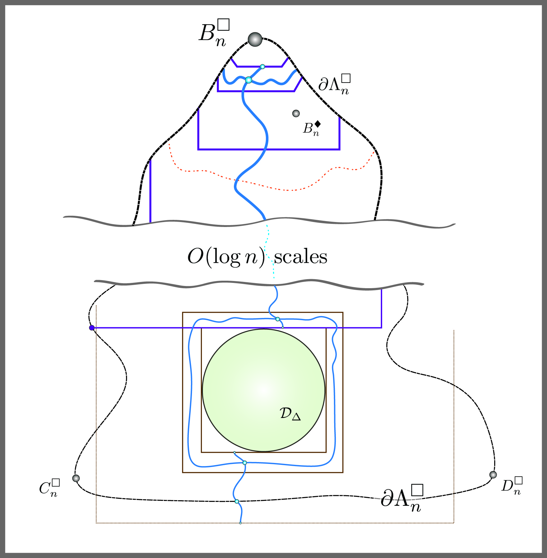
Figure 2: Preliminary circuit element “inside” $B_{n}$ plus connection to $[C_{n}^{\square},D_{n}^{\square}]$ boundary – first via intermediate scales then to the vicinity of $\mathcal{D}_{\Delta}$ and the rest by large–scale events – prevents the occurrence of of the yellow circuit described. If there are fewer than $\gamma\log n$ intermediate scales then this circuit would have substantive probability.

First we have that by Lemma 3.5 and Definition 3.8 that e.g., $|S_{B}^{\square}(B_{n})|\gtrsim 1-n^{-a_{4}}-n^{-\beta}\gtrsim 1-n^{-a_{4}}$. (Recall that $\beta>a_{3}>a_{4}$ and $S_{B}^{\square}(B_{n})$ is the probability of a yellow crossing from $(B_{n}^{\square},C_{n}^{\square})$ to $(D_{n}^{\square},B_{n}^{\square})$ separating $B_{n}$ from $(C_{n}^{\square},D_{n}^{\square})$.) On the other hand, let us consider the “last” Harris ring separating $B_{n}$ from $B_{n}^{\square}$ which forms a conduit between $[D_{n}^{\square},B_{n}^{\square}]$ and $[B_{n}^{\square},C_{n}^{\square}]$, c.f., Theorem 3.10, item 3; we may enforce a crossing in this conduit with probability $\vartheta$ (as in Theorem 3.10) and then via a box construction and a “large scale” crossing (as appears below in the proof of Lemma 3.12) the said crossing can be connected to $[C_{n}^{\square},D_{n}^{\square}]$ in blue. This construction procedure is illustrated in Figure 2. Therefore, if the number of Harris rings enclosing $B_{n}$ were less than $\gamma\cdot\log n$, then there would be some $V>0$ such that the journey from the vicinity of $B_{n}$ to $[C_{n}^{\square},D_{n}^{\square}]$ can occur at a probabilistic cost in excess of $n^{-\gamma V}$.

Since such a blue connection renders a yellow version of the event $\mathbb{S}_{B}^{\square}(B_{n})$ impossible, we conclude that there must be more than $a_{4}/V$ Harris rings enclosing $B_{n}$, for $n$ sufficiently large. Similar arguments yield the result also for $C_{n},D_{n}$. ∎

More generally, we have the following description of the distance between $\partial\Omega_{n}^{\square}$ and $\partial\Omega_{n}$:

Lemma 3.12

Let $s\in\partial\Omega_{n}$ and $z\equiv z(s)$ the point on $\partial\Omega_{n}^{\square}$ which is closest to $s$ (in the Euclidean distance). Then there exists some $\kappa>0$ such that in the Harris system stationed at $z$, there are at least $\kappa\cdot\log n$ Harris rings that enclose $s$.

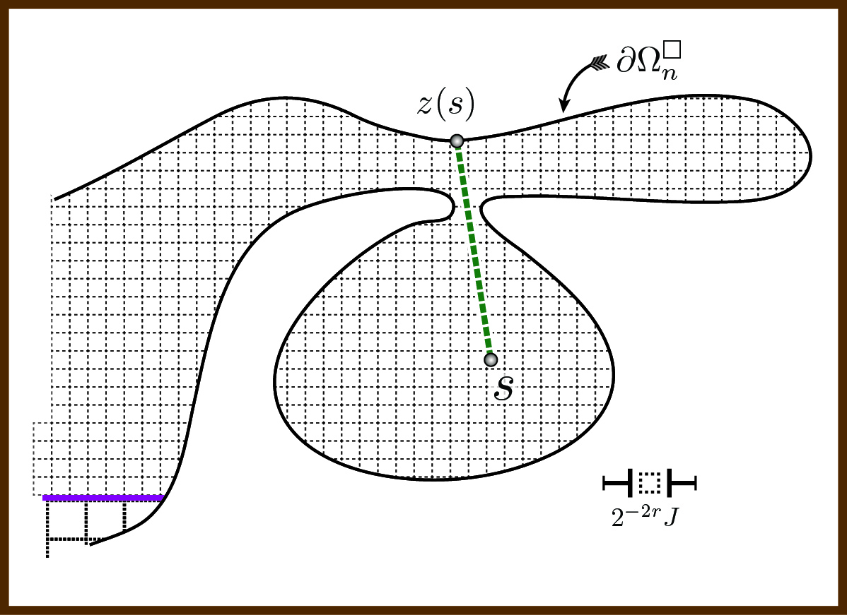
Figure 3: Case 3 of Lemma 3.12: if the box containing $s$ is separated from the main percolating cluster of full boxes (of scale $2^{-2r}\cdot J$) associated with its ring by a partial box then, necessarily, $z$ could not be the point on $\partial\Omega_{n}^{\square}$ which is closest to $s$.

Proof.

Let us set $\lambda:=\mbox{dist}(s,z)$. First, logically speaking, we must rule out the possibility that $s$ is outside the Harris system stationed at $z$ altogether: if this were true, then it would imply that $\mbox{dist}(s,\partial\Omega_{n}^{\square})=\lambda>\frac{1}{2}\Delta$ (since Harris circuits plug into $\partial\Omega_{n}^{\square}$ the point $s$ can only be outside the Harris system at $z$ altogether if it is “beyond” the last Harris segment which parallels $\partial\mathcal{D}_{\Delta}$; see Theorem 3.10) which then readily implies that all of the $S$–functions are of order unity: indeed, in this case $S_{B}^{\square}(s),S_{C}^{\square}(s)$ and $S_{D}^{\square}(s)$ can all be bounded from below by large scale events of order unity (consider e.g., the crossing of a suitable annulus whose aspect ratio is order unity with $s$ on the boundary of the inner square and the outer square touching $\partial\Omega_{n}^{\square}$ (from inside $\Omega_{n}^{\square}$) together with yet another couple of crossings from the inner square of this annulus to a larger rectangle which encloses all of $\Omega_{n}^{\square}$) which would place $s$ well away from the boundary of $\Omega_{n}$ by Definition 3.8 and Lemma 3.5. Thus $s$ is in a Harris ring of $z$.

If the separation – measured in number of Harris rings – between $s$ and $\mathcal{D}_{\Delta}$ is not so large, then we will show that $|S_{n}^{\square}(z)|$ is larger than a small inverse power of $n$. We will accomplish this by constructing configurations which lead to the occurrence of all three events corresponding to $S_{B}^{\square},S_{C}^{\square},S_{D}^{\square}$ with sufficiently large probability. To this end we will make detailed use of the Harris system.

Let $J$ denote the separation distance of the Harris segments which form the ring containing $s$ and let $r>0$ be as given in Theorem 3.10. Now note that if the statement of the lemma were false, then there would be an abundance of Harris rings separating $z$ from $s$, which will enable us to construct a path “beneath” $s$ to yield the events $\mathbb{S}_{B}^{\square},\mathbb{S}_{C}^{\square},\mathbb{S}_{D}^{\square}$. Consider the boxes of size $2^{-2r}\cdot J$ which grid the ring containing $s$. Let us observe that there are three cases: 1) the main type, $s$ is contained in a full box which is connected to the cluster which percolates through the ring (see Theorem 3.10, item 1); 2) the partial type, meaning that $s$ is in a partial box, i.e., a box intersected by $\partial\Omega_{n}^{\square}$; 3) $s$ is in a full box which is separated from the cluster of main types of percolating boxes by a partial box.

Let us rule out the possibility of 2) and 3). Case 2) is impossible since it implies that $\mbox{dist}(s,z)=\mbox{dist}(s,\partial\Omega_{n}^{\square})\leq 2^{-2r}\cdot J$ which (see Theorem 3.10, items 1 and 2) necessarily implies that $z$ and $s$ are in the same ring. But, supposing they do reside in the same ring then with probability in excess of (some constant times) $1-n^{-\Gamma}$, with $\Gamma$ as in Theorem 3.10, the occurrence or not of the events contributing to $S_{B}^{\square},S_{C}^{\square},S_{D}^{\square}$ would be the same for both $s$ and $z$ (c.f., the proof of Proposition 3.15 below). Then by Lemma 3.5 and Definition 3.8, it would the case that $|S_{n}^{\square}(z)-S_{n}^{\square}(s)|\gtrsim n^{-a_{4}}-n^{-\beta}$, which is a contradiction if $a_{4},\beta$ are appropriately chosen relative to $\Gamma$.

Similar reasoning shows that 3) is also not possible: indeed, since $z$ is the closest point to $s$, $z$ and $s$ must lie along a straight line segment which lies in $\Omega_{n}^{\square}$ and this segment must pass through the partial box in question (i.e., the “bottleneck”; we emphasize here that we are considering the Harris system centered at $z$) which separates $s$ from the connected component of boxes which percolate through the ring. From previous considerations regarding $2^{-2r}J$ (the scale of the boxes) versus $\mbox{dist}(s,z)$, it is clear that there is a point on $\partial\Omega_{n}^{\square}$ within this partial box which is closer to $s$ than $z$, a contradiction. These considerations are illustrated in Figure 3.

Thus, we find $s$ in the main percolating component of boxes. For convenience, we focus on the sub–case where the box containing $s$ is separated from $\partial\Omega_{n}^{\square}$ by at least one layer of full boxes. Indeed, the complementary sub–cases are easily handled by arguments similar to those which dispensed with cases 2) and 3).

We shall now proceed to construct, essentially by hand, any of the events $\mathbb{S}_{B}^{\square}(s)$, $\mathbb{S}_{C}^{\square}(s)$ or $\mathbb{S}_{D}^{\square}(s)$ corresponding to the functions $S_{B}^{\square},S_{C}^{\square},S_{D}^{\square}$, respectively, with “unacceptably large” probability.

It is understood that the constructions that follow utilize the main body of boxes percolating through a given Harris ring fragment, as detailed in Theorem 3.10, item 1. Ultimately we will be constructing two (disjoint) paths. E.g., for the $\mathbb{S}_{B}^{\square}(s)$ event, one path from the vicinity of $s$ to the $[B^{\square}_{n},C^{\square}_{n}]$ boundary and the other from the vicinity of $s$ to the $[D^{\square}_{n},B^{\square}_{n}]$ boundary. While not strictly necessary, it is slightly more convenient to construct the “bulk” of both paths at once. Therefore, we shall undertake a double bond construction. For further convenience, we will base our construction on $3\times 1$ bond events which will be described in the next paragraph.

We remark, again, that arguments of this sort have appeared before, e.g., at least as far back as [1], so we will be succinct in our descriptions. The events are described as follows: let us assume, for ease of exposition, that three neighboring boxes form a horizontal $3\times 1$ rectangle. The bond event – in yellow – would then consist of two disjoint left–right yellow crossings of the $3\times 1$ rectangle together with two disjoint top–bottom yellow crossings in each of the outer two squares, as is illustrated in Figure 4, it is seen that if a pair of such rectangles overlap on an end–square, and the bond event occurs for both of them, then, regardless of the orientations, there are two disjoint yellow paths which transmit from the beginning of one to the end of the other. I.e., these “bonds” have the same connectivity properties as the bonds of $\mathbb{Z}^{2}$ and provide us with double paths.

Starting with the square containing $s$ we may suppose there is (or construct) a yellow ring in the eight boxes immediately surrounding and encircling this square. Via the bond events just described, we connect this encircling ring to the outward boundary of the Harris annulus to which $s$ belongs. Each of these events – which are positively correlated – incurs a certain probabilistic cost. However, it is observed, with emphasis, that since the relative scales of the Harris ring and the bonds used in the construction are fixed independent of the actual scale, the cost may be bounded by a number independent of the actual scale.

Similarly, we may use the bonds to acquire a double path across the next (outward) ring and the two double paths may be connected to form a continuing double path by explicit use of a “patch” consisting of the smaller of the two bond types. Again, since the ratio of scales of (boxes of) successive Harris rings are uniformly bounded above and below, the probabilistic cost does not depend on the actual scale. The procedure of double crossing via bond events and patches can be continued till the boundary of $\mathcal{D}_{\Delta}$ is reached; thereupon, treating $\mathcal{D}_{\Delta}$ and its vicinity as an annulus in its own right, the two paths can be connected to separate boundaries at an additional cost of order unity.

Now let us assume for the moment that $s\in[B_{n},C_{n}]$, so that by Lemma 3.5 and Definition 3.8 it is the case that $S_{D}^{\square}(s)\leq C\cdot(n^{-a_{4}}+n^{-\beta})$ for some constant $C>0$, so denoting by $\text{e}^{-V}$ (for some $V>0$) the uniform bound on the cost of one patch and one annular crossing via the double bonds, if $\kappa>0$ is sufficiently small so that $\text{e}^{-\kappa V\log n}=n^{-\kappa V}>C\cdot(n^{-a_{4}}+n^{-\beta})$, then it is not possible that $s\in[B_{n},C_{n}]$. By cyclically permuting the relevant $B,C,D$ labels, the cases where $s\in[C_{n},D_{n}]$ and $s\in[D_{n},B_{n}]$ follow similarly. ∎

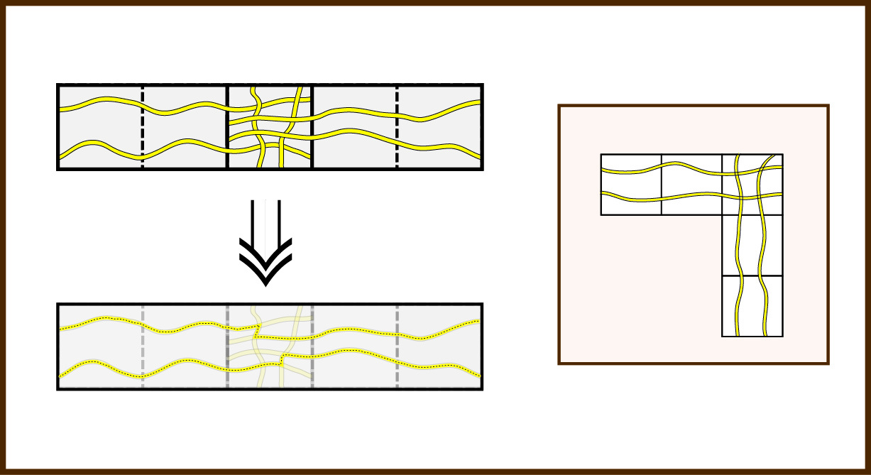
Figure 4: Two pairs of disjoint left–right crossings in successive overlapping $3\times 1$ blocks together with two disjoint top–bottom crossings in the common square allow for the continuation of two disjoint paths. Not all crossings described in the bond event are shown. Note, as illustrated in the insert that, in the case of right angle continuations, the additional paths in the overlap block are superfluous.

The ensuing arguments will require an auxiliary point somewhat inside $\Omega_{n}$, which we will denote $A_{n}^{\diamondsuit}$:

Definition 3.13.

Let $\Omega_{n}^{\square},\Omega_{n}$, etc., be as described. Let $\eta>0$ be a number to be specified in Proposition 3.14. Then we let $A_{n}^{\diamondsuit}$ be a point in the Harris ring of the Harris system stationed at $A_{n}^{\square}$ which is separated from $\mathcal{D}_{\Delta}$ by $\eta\cdot\log n$ Harris segments. Moreover, $A_{n}^{\diamondsuit}$ is in the center of a box which belongs to the connected component of the boxes which percolate through the relevant ring (see the description in Theorem 3.10, item 1) as in the proof of Lemma 3.12.

Proposition 3.14

There exists some $\eta>0$ such that if $A_{n}^{\diamondsuit}$ is as in Definition 3.13, then there exists some $\gamma>0$ such that

1. $|S_{n}^{\square}(A_{n}^{\square})-S_{n}^{\square}(A_{n}^{\diamondsuit})|\lesssim n^{-\gamma}$;

2. $|H_{n}^{\square}(A_{n}^{\square})-H_{n}^{\square}(A_{n}^{\diamondsuit})|\lesssim n^{-\gamma}$;

In particular, with appropriate choice of $\gamma$, $A_{n}^{\diamondsuit}$ is strictly inside $\Omega_{n}$.

Proof.

First let us establish item 1. It is claimed that for any configuration in which the event $\mathcal{A}(A_{n}^{\diamondsuit})$ – of a blue circuit connecting $[D_{n}^{\square},A_{n}^{\square}]$ to $[A_{n}^{\square},B_{n}^{\square}]$ which surrounds both $A_{n}^{\square}$ and $A_{n}^{\diamondsuit}$ (as described in Theorem 3.10, item 3) – occurs, the indicator function of the yellow version of $\mathbb{S}_{n}^{\square}(A_{n}^{\square})$ is equal to that of $\mathbb{S}_{n}^{\square}(A_{n}^{\diamondsuit})$. Indeed, for the $S_{C}^{\square}$–component, which always vanishes for $A_{n}^{\square}$, the requisite event in yellow is directly obstructed by the blue paths of $\mathcal{A}(A_{n}^{\diamondsuit})$. As for the rest, for either of the differences in the $B$ or $D$ components to be non–zero, there must be a long yellow path separating $A_{n}^{\square}$ from $A_{n}^{\diamondsuit}$ heading to a distant boundary, but this separating path is preempted by the blue event $\mathcal{A}(A_{n}^{\diamondsuit})$. We may thus conclude that

$$\mathbb{E}(|\mathbb{I}_{\mathbb{S}_{n}^{\square}(A_{n}^{\square})}-\mathbb{I}_{\mathbb{S}_{n}^{\square}(A_{n}^{\diamondsuit})}|\mid\mathcal{A}(A_{n}^{\diamondsuit}))=0$$ (3.5)

(where $\mathbb{I}_{(\bullet)}$ denotes the indicator) which together with Lemma 3.12 and Theorem 3.10, item 3 gives the result.

As for item 2, recalling the discussion near the end of the proof of Theorem 3.3, we may consider $\Omega_{n}^{\square}$ to be a fixed continuum domain and, e.g., for $N\geq n$, the domain $\Omega_{n,N}^{\square}$ to be its canonical approximation (together with appropriate approximations for the marked points $A_{n}^{\square},B_{n}^{\square}$, etc.) for a percolation problem at scale $N^{-1}$. We will consider the corresponding CCS–functions $S_{n,N}^{\square}$ on the domains $\Omega_{n,N}^{\square}$.

Let us now argue that the arguments for item 1 persist, uniformly, for all $N$ sufficiently large. First, it is emphasized that all the results follow from the occurrence of paths in each Harris ring, which has probability uniformly bounded from below. We claim that this remains the case for percolation performed at scale $N^{-1}$. Indeed, while the scales of the Harris rings were constructed existentially to ensure uniform bounds on crossings at scale $n^{-1}$, it is recalled that these rings are gridded by boxes of scale $2^{-2r}$ relative to the rings themselves (see Theorem 3.10, item 1). Thence, using uniform probability crossings in squares/rectangles, etc., the necessary crossings can be constructed by hand as in e.g., the proof of Lemma 3.12.

For the last statement, we invoke an argument similar to that in the proof of Lemma 3.12. Recapitulating the construction, we acquire a lower bound on the probability of occurrence of any of the events associated with the $S$–functions for $A_{n}^{\diamondsuit}$. Finally, since $S_{n}^{\square}$ is close to $F_{n}^{\square}$ by Lemma 3.5 the latter of which is used to define $\partial\Omega_{n}$, with an appropriate choice of power of $n$ (i.e., $\gamma$) $A_{n}^{\diamondsuit}$ can be placed in the interior of $\Omega_{n}$. ∎

Proposition 3.15

There exists some $a_{5}>0$ such that

$$|F_{n}^{\square}(A_{n}^{\diamondsuit})-S_{n}^{\square}(A_{n}^{\square})|\leq n^{-a_{5}}.$$

Proof.

This follows immediately from Proposition 3.14, item 1 and Lemma 3.5. ∎

Finally, we will need a result concerning the conformal maps $H_{n}$ and $H_{n}^{\square}$. First we state a distortion estimate:

Lemma 3.16

Let $\epsilon>0$ and let $K\subseteq\mathbb{T}$ be a domain whose boundary is a Jordan curve such that the sup–norm distance between $\partial K$ and $\partial\mathbb{T}$ is less than $\epsilon$. We consider $K$ to be a conformal triangle with some marked points $K_{B},K_{C},K_{D}$ such that $|K_{B}-1|<\epsilon$, $|K_{C}-\tau|<\epsilon$, $|K_{D}-\tau^{2}|<\epsilon$, and let $g_{K}$ denote the conformal map from $K$ to $\mathbb{T}$ mapping $(K_{B},K_{C},K_{D})$ to $(1,\tau,\tau^{2})$. Then for $z\in K$ it is the case that

$$|g_{K}(z)-z|\lesssim[\epsilon\cdot\log(1/\epsilon)]^{1/3}.$$

Proof.

The result for the disk (without the power of 1/3) is a classical result going back to Marchenko (for a statement see [16], Section 3) and of course, we can transfer our hypotheses to the disk by applying a conformal map $\phi$, which maps $\mathbb{T}$ to the unit disk such that $\phi(0)=0$. The map $\phi$ does not increase the distances, because it is smooth up to the boundary everywhere but at $1$, $\tau$, and $\tau^{2}$, where it behaves locally like $\epsilon^{3}$, which in fact only decreases the distances.

We are almost in a position to directly apply Marchenko’s Theorem except for a few caveats. First of all Marchenko’s Theorem requires a certain geometric condition on the tortuosity of the boundary of $K$, which is manifestly satisfied under the assumption that $\partial K$ and the boundary of the triangle are close in the sup–norm distance.

Secondly, Marchenko’s Theorem is stated for some map $f_{K}$ with $f_{K}(0)=0$ and $f^{\prime}_{K}(0)>0$, and we have a possibly different normalization. Specifically, we have some map $G_{K}:\phi(K)\rightarrow\mathbb{D}$ so that $\phi^{-1}\circ G_{K}\circ\phi=g_{K}$, so it suffices to check that $G_{K}$ has approximately the correct normalizations (indeed, the conformal self–map of the unit disc mapping a point $a$ to the origin takes the form  $e^{i\theta}\cdot\left(\frac{z-a}{1-\bar{a}z}\right)$).

Since $\phi(0)=0$ and $1+\tau+\tau^{2}=0$ it is the case that $\phi^{-1}((1-\epsilon)\cdot\phi(K_{B}+K_{C}+K_{D}))$ is close to 0 and also close to $w:=\phi^{-1}((1-\epsilon)\cdot\phi(K_{B}))+\phi^{-1}((1-\epsilon)\cdot\phi(K_{C}))+\phi^{-1}((1-\epsilon)\cdot\phi(K_{D}))$; since it is also the case that $g_{K}(K_{B})+g_{K}(K_{C})+g_{K}(K_{D})$ is close to 0, we have that $G_{K}(w)$ is close to 0. So we now have that $G_{K}(z)$ is close to some $e^{i\theta}z$ for some fixed $\theta$. But since $\phi(K_{B})$ is close to $\phi(1)$, and so $z_{0}:=\phi^{-1}((1-\epsilon)\phi(K_{B}))$ is close to both 1 and $e^{-i\theta}\cdot G_{K}(1)$, it follows that $|e^{i\theta}-1|\lesssim\epsilon\cdot\log(1/\epsilon)$.

Finally, in transferring the result back to the triangle, the behavior near the vertices of the triangle requires us to replace the distances by their cube roots. ∎

Remark 3.17.

We remark that for our purposes, we can in fact avoid the fractional power: indeed, we shall only use this result at the point $A_{n}^{\diamondsuit}$, which we remind the reader is chosen to be in the Harris system stationed at $A_{n}^{\square}$ and by Lemma 5.14 we may assert that it is within a fixed small neighborhood of $A_{n}^{\square}$ and therefore outside fixed neighborhoods of the other marked points.

Lemma 3.18

There exists some $a_{6}>0$ such that for all $n$ sufficiently large,

$$|H_{n}(A_{n}^{\diamondsuit})-H_{n}^{\square}(A_{n}^{\diamondsuit})|\lesssim n^{-a_{6}}.$$

Proof.

Denoting by $G_{n}$ the conformal map mapping $H_{n}^{\square}(\Omega_{n})$ to $\mathbb{T}$ with the points $(H_{n}^{\square}(B_{n}),H_{n}^{\square}(C_{n})$, $H_{n}^{\square}(D_{n}))$ mapping to the points $(1,\tau,\tau^{2})$, we have by uniqueness of conformal maps that

$$H_{n}=G_{n}\circ H_{n}^{\square}.$$

The stated result will follow from Lemma 3.16, and in order to utilize this lemma, we need to verify that $(H_{n}^{\square}(B_{n}),H_{n}^{\square}(C_{n}),H_{n}^{\square}(D_{n}))$ is close to $(1,\tau,\tau^{2})$ and to show that the sup–norm distance between $\partial[H_{n}^{\square}(\partial\Omega_{n})]$ and $\partial\mathbb{T}$ is less than $n^{-\gamma}$ for some $\gamma>0$. The first statement is a direct consequence of Proposition 3.11: since $O(\log n)$ Harris rings surround both $B_{n}$ and $B_{n}^{\square}$, by an argument as in the proof of Proposition 3.14, their $S_{n}^{\square}$ values differ by an inverse power of $n$ and the result follows since $S_{n}^{\square}(B_{n}^{\square})\equiv 1$; similar arguments yield the result for $C_{n},D_{n}$.

As for the second statement, first we have by Lemma 3.5 and Lemma 3.9 that the distance between $\partial[S_{n}^{\square}(\partial\Omega_{n})]$ and $\partial\mathbb{T}$ is less than (some constant times) $n^{-a_{4}}+n^{-\beta}$; we emphasize that here we in fact have closeness in the sup–norm since both lemmas yield pointwise estimates. Next, as near the end of the proof of Theorem 3.3, we may consider $\Omega_{n}^{\square}$ to be a fixed continuum domain and, e.g., for $N\geq n$, the domain $\Omega_{n,N}^{\square}$ to be its canonical approximation (together with appropriate approximations for the marked points $A_{n}^{\square},B_{n}^{\square}$, etc.) for a percolation problem at scale $N^{-1}$. We will consider the corresponding CCS–functions $S_{n,N}^{\square}$ on the domains $\Omega_{n,N}^{\square}$.

We claim that there exists some $\gamma>0$ such that uniformly in $N$ for $N$ sufficiently large, the sup–norm distance between $\partial[S_{n,N}^{\square}(\partial\Omega_{n})]$ and $\partial\mathbb{T}$ is less than $n^{-\gamma}$. Indeed, from Lemma 3.12, we know that for each point $s$ on $\partial\Omega_{n}$, there are $\kappa\cdot\log n$ Harris rings stationed at $z(s)$ which separate it from the central region $\mathcal{D}_{\Delta}$. While by fiat $S_{n,N=n}^{\square}(\partial\Omega_{n})$ is close to $\partial\mathbb{T}$, we shall reprove this using the Harris systems since we require an estimate which is uniform in $N$. We start with the following observation concerning the central region $\mathcal{D}_{\Delta}$:

Claim. For $n$ sufficiently large, with probability of order unity independent of $n$, there are monochrome percolative connections (in blue or yellow) between $\mathcal{D}_{\Delta}$ and any or all of the three boundary segments.

Proof of Claim. Consider the domain $\Omega$ with marked points $B,C,D$, viewed as a conformal triangle. It is recalled that $\mathcal{D}_{\Delta}$ is roughly half the size of the largest circle which can be fit into $\Omega$. Let us focus on two of the three marked points, say $B$ and $D$. We now mark two boundary points on $\mathcal{D}_{\Delta}$ and denote them by $b$ and $d$ and consider two disjoint curves which join $B$ to $b$ and $D$ to $d$, thereby forming a conformal rectangle. Since the aspect ratio of the said rectangle is fixed, it therefore follows, by convergence to Cardy’s Formula, that for $n$ sufficiently large, there is a uniform lower bound on the probability of a discrete realization of the desired connection. Similar arguments apply to the other two boundary segments. ∎

Claim. Consider $s\in\partial\Omega_{n}$ and the Harris rings from the Harris system stationed at $z(s)\in\partial\Omega_{n}^{\square}$ which also enclose $s$ as in Lemma 3.12. Without loss of generality, we may assume that $z(s)\in[B_{n}^{\square},D_{n}^{\square}]$. Then there exists some fixed constant $\Upsilon<\infty$ such that all but $\Upsilon$ of the Harris segments have at least one endpoint on $[B_{n}^{\square},D_{n}^{\square}]$. Moreover, among these, either the other endpoint of the Harris segment is also on $[B_{n}^{\square},D_{n}^{\square}]$ or the existence of the corresponding path event within this Harris segment achieves $\mathbb{S}_{B}^{\square}$ or $\mathbb{S}_{D}^{\square}$ (which, we remind the reader, are the percolation events defining $S_{D}^{\square}$ and $S_{B}^{\square}$, respectively) for both $s$ and $z(s)$. Similar statements hold if $z$ belongs to the other boundary segments.

Proof of Claim. Let us first rule out the possibility that too many Harris segments have endpoints on $[B_{n}^{\square},C_{n}^{\square},D_{n}^{\square}]$. It is noted that each Harris segment of this type in fact separates all of $[B_{n}^{\square},D_{n}^{\square}]$ from $\mathcal{D}_{\Delta}$. Thus, if there are say $\Upsilon$ such Harris segments, then the probability of a connection between $\mathcal{D}_{\Delta}$ and $[B_{n}^{\square},D_{n}^{\square}]$ would be less than $(1-\vartheta)^{\Upsilon}$, with $\vartheta>0$ as in Theorem 3.10. It follows from the previous claim that $\Upsilon$ cannot scale with $n$.

Finally, if there are too many Harris segments with one endpoint on $[B_{n}^{\square},D_{n}^{\square}]$, but accomplishes neither $\mathbb{S}_{B}^{\square}$ nor $\mathbb{S}_{D}^{\square}$, then necessarily the other endpoint must be on $[B_{n}^{\square},C_{n}^{\square}]$ or $[C_{n}^{\square},D_{n}^{\square}]$ in such a way that the Harris segment separates $\mathcal{D}_{\Delta}$ from $[B_{n}^{\square},C_{n}^{\square}]$ or $[C_{n}^{\square},D_{n}^{\square}]$. The same reasoning as in the above paragraph then implies that this also cannot occur “too often”. For illustrations of some of these cases, see Figure 5. ∎

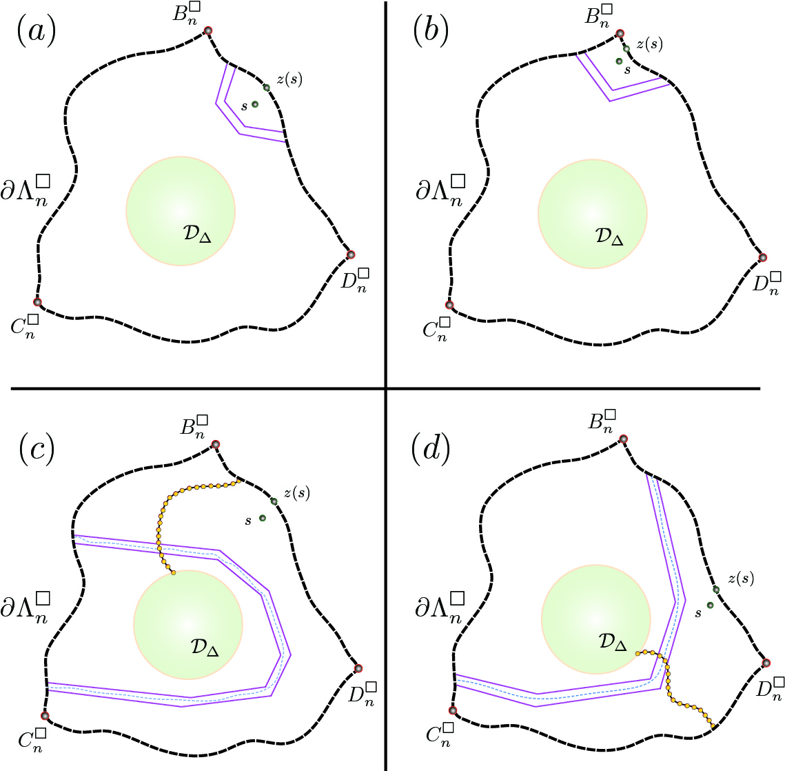
Figure 5: (a) and (b): Harris annular segment of the type envisioned for $s\in\partial\Omega_{n}$ and $z(s)\in[B_{n}^{\square},D_{n}^{\square}]$; in case (b), it so happens that $z(s)$ and $B_{n}^{\square}$ are close. (c) and (d): since yellow paths indicated in these illustrations represent typical large scale events, there cannot be too many Harris rings of the contrary type.

We also note that there cannot be Harris segments of conflicting “corner types” (e.g., $[D_{n}^{\square},B_{n}^{\square}]$ to $[B_{n}^{\square},C_{n}^{\square}]$ and $[B_{n}^{\square},C_{n}^{\square}]$ to $[C_{n}^{\square},D_{n}^{\square}]$) since the Harris segments are topologically ordered and cannot intersect one another.

We can now acquire the needed conclusion that the Harris rings themselves force $S_{n,N}^{\square}(s)$ to be close to $\partial\mathbb{T}$. The essence of the argument can be captured by the (redundant) case $N=n$, so let us proceed. Consider then $s\in\partial\Omega_{n}$ and the Harris system stationed at $z(s)\in\partial\Omega_{n}^{\square}$ as above which, without loss of generality, we assume to be in $[B_{n}^{\square},D_{n}^{\square}]$. Then we claim that $|S_{n}^{\square}(z(s))-S_{n}^{\square}(s)|\lesssim n^{-\kappa}$. Indeed, from the previous claim, all but $\Upsilon$ of the Harris segments have beginning and ending points on $\partial\Omega_{n}^{\square}$ which are such that conditioned on the existence of paths of the appropriate color within these segments, the indicator functions of all $S_{n}^{\square}$–events are the same value for both $s$ and $z(s)$.

Let us now argue that the above argument persists, uniformly, for all $N$ sufficiently large. First, it is emphasized that all arguments follow from the occurrence of paths in each Harris ring, which has probability uniformly bounded from below. We claim that this remains the case for percolation performed at scale $N^{-1}$. Indeed, let us again recall that these rings are gridded by boxes of scale $2^{-2r}$ relative to the rings themselves (see Theorem 3.10) and using uniform probability of crossings in squares/rectangles, etc., which is characteristic of critical 2D percolation problems, the necessary crossings can be constructed by hand as in e.g., the proof of Lemma 3.12.

Now by convergence to Cardy’s Formula (or rather, the statement that the CCS–function converges uniformly on compact sets to the conformal map to $\mathbb{T}$) it is the case that $S_{n,N}^{\square}(s)\rightarrow H_{n}^{\square}(s)$. Uniformity in $s$ follows from the fact that $\overline{\Omega_{n}}\subseteq\Omega_{n}^{\square}$ is a fixed (for $n$ fixed) compact set, c.f., Section 5 in [5]. We conclude therefore that each point on $\partial\Omega_{n}$ maps to a point sufficiently close to $\partial\mathbb{T}$, and since $\partial[H_{n}^{\square}(\partial\Omega_{n})]$ is a curve, it easily follows that the Hausdorff distance is small.

However, we require the stronger statement that the relevant objects are close in the sup–norm (i.e., in $d_{\rm sup}(\cdot,\cdot)$). We will now strengthen the above arguments to acquire this conclusion. Let us define the set of all points which are chosen as the $z(s)$ (the closest point to $s$) for some $s$ in $\langle\partial\Omega_{n}\rangle_{N}$ (the approximation to $\partial\Omega_{n}$ at scale $N^{-1}$):

$$\mathcal{Z}_{N}:=\{z\in\partial\Omega_{n,N}^{\square}\mid\exists s\in\langle\partial\Omega_{n}\rangle_{N},z=z(s)\}.$$

Let us first observe that a priori $S_{n,N}^{\square}(\mathcal{Z}_{N})$ is a discrete set of points on $\partial\mathbb{T}$ which we may consider to be a curve by linear interpolation. For simplicity let us consider the portion of $\partial\mathbb{T}$ corresponding to the $[C,D]$ boundary, i.e., the vertical segment connecting $\tau$ and $\tau^{2}$. Let us focus attention on $S_{n,N}^{\square}([C_{n,N}^{\square},D_{n,N}^{\square}]\cap\mathcal{Z}_{N})$. By monotonicity of crossing probabilities, it is the case that these points are ordered along the vertical segment.

Now our contention is that there are no substantial gaps between successive points:

Claim. Let $s\in\langle\partial\Omega_{n}\rangle_{N}$ and $z(s)$ be as described. Let $\nu>0$ be such that the inequality $n^{-\nu}\gg n^{-\kappa}$ is sufficiently strong, as will emerge in the proof, where $\kappa$ as above is such that $|S_{n,N}^{\square}(s)-S_{n,N}^{\square}(z(s))|\lesssim n^{-\kappa}$. Then for all $N>n$, it is the case that the maximum separation between successive points of $S_{n,N}^{\square}([C_{n,N}^{\square},D_{n,N}^{\square}]\cap\mathcal{Z}_{N})$ is less than $n^{-\nu}$, with $\mathcal{Z}_{N}$ as described.

Proof of Claim. Suppose there are two points $x_{1},x_{2}\in[C_{n,N}^{\square},D_{n,N}^{\square}]\cap\mathcal{Z}_{N}$, say with $S_{n,N}^{\square}(x_{1})$ below $S_{n,N}^{\square}(x_{2})$, which are separated by a gap in excess of $n^{-\nu}$. Let us denote by $s_{1},s_{2}\in\langle\partial\Omega_{n}\rangle_{N}$ the points corresponding to $x_{1},x_{2}$, respectively. Next consider the $\frac{1}{4}\cdot n^{-\nu}$ neighborhoods of $S_{n,N}^{\square}(s_{1})$ and $S_{n,N}^{\square}(s_{2})$ and consider the points in $\partial\Omega_{n}$ “between” $s_{1}$ and $s_{2}$. There must be points between $s_{1}$ and $s_{2}$ since $|S_{n,N}^{\square}(s_{1})-S_{n,N}^{\square}(s_{2})|\gtrsim n^{-\nu}-2\cdot n^{-\kappa}$. So if these points were neighbors, by standard critical percolation arguments, the difference between their $S_{n,N}^{\square}$ values must be small and the above inequality would render this difference unacceptably large, for $\nu$ appropriately chosen.

If these points all have $S_{n,N}^{\square}$–value which lie in the $\frac{1}{4}\cdot n^{-\nu}$ neighborhoods described above, then there would be a neighboring pair whose $S_{n,N}^{\square}$ values are separated by $\frac{1}{2}\cdot n^{-\nu}$, which would again be unacceptably large. We conclude therefore that there exists some point between $s_{1}$ and $s_{2}$ with $S_{n,N}^{\square}$ value outside these neighborhoods and therefore a point in $\mathcal{Z}_{N}$ whose $S_{n,N}^{\square}$ value lies between those of $x_{1}$ and $x_{2}$. This is a contradiction. ∎

Finally, let us describe the parametrization. First we denote by $U_{N}$ the number of points in $\mathcal{Z}_{N}$ and then we may parametrize say the vertical portion of $\partial\mathbb{T}$ by having, for $t=j$, the curve on the $j^{\text{th}}$ site of $\mathcal{Z}_{N}$ and linearly interpolating for the non–integer times. Similarly, we parametrize the corresponding portion of $S_{n,N}^{\square}(\langle\partial\Omega_{n}\rangle_{N}$, so that pairs of points at integer times correspond to their $s,z(s)$ pair. The above claim then implies that with this parametrization, the two curves are within $n^{-\nu}$ at all times. We have verified that $S_{n,N}^{\square}(\langle\partial\Omega_{n}\rangle_{N})$ is sup–norm close to $\partial\mathbb{T}$, uniformly in $N$.

The stated result now follows from Lemma 3.16. ∎

Proof of the Main Theorem. The required power law estimate for the rate of convergence of crossing probabilities now follows by concatenating the various theorems, propositions and lemmas we have established. Let us temporarily use the notation $A\sim B$ to mean that $A$ and $B$ differ by an inverse power of $n$.

Starting with $S_{n}(A_{n})$, we have that $S_{n}(A_{n})\sim S_{n}^{\square}(A_{n}^{\square})$ by Theorem 3.3; $S_{n}^{\square}(A_{n}^{\square})\sim S_{n}^{\square}(A_{n}^{\diamondsuit})$ by Proposition 3.14, item 1; $S_{n}^{\square}(A_{n}^{\diamondsuit})\sim F_{n}^{\square}(A_{n}^{\diamondsuit})$ by Lemma 3.5; $F_{n}^{\square}(A_{n}^{\diamondsuit})\sim H_{n}(A_{n}^{\diamondsuit})$ by Lemma 3.9; $H_{n}(A_{n}^{\diamondsuit})\sim H_{n}^{\square}(A_{n}^{\diamondsuit})$ by Lemma 3.18; $H_{n}^{\square}(A_{n}^{\diamondsuit})\sim H_{n}^{\square}(A_{n}^{\square})$ by Proposition 3.14, item 2; finally, $H_{n}^{\square}(A_{n}^{\square})\sim H(A)$ by Theorem 3.3.

∎

4 $\sigma$–Holomorphicity

The main goal in this section is to establish the so–called Cauchy integral estimates which is one of the more technical aspects required for the proof of Lemma 3.5. We will address such issues in somewhat more generality than strictly necessary by extracting the two properties of functions of the type $S_{n}(z)$ which are of relevance: i) Hölder continuity and ii) that their discrete (closed) contour integrals are asymptotically zero as the lattice spacing tends to zero. As for the latter, it should be remarked that the details of how our particular $S_{n}(z)$ exhibits its cancelations on the microscopic scale can be directly employed to provide the Cauchy–integral estimates.

4.1 $(\sigma,\rho)$–Holomorphicity

As a starting point – and also to fix notation – let us review the concept of a discrete holomorphic function on a hexagonal lattice. Let $\mathbb{H}_{\varepsilon}$ denote the hexagonal lattice at scale $\varepsilon$, e.g., the length of the sides of each hexagon is $\varepsilon$, so we envision $\varepsilon=n^{-1}$, where the hexagons are oriented horizontally (i.e., two of the sides are parallel to the $x$–axis). For now, let $\Lambda_{\varepsilon}$ denote any collection of hexagons and $Q:\Lambda_{\varepsilon}\to\mathbb{C}$ a function on the vertices of $\Lambda_{\varepsilon}$. For each pair of adjacent vertices in $\Lambda_{\varepsilon}$ let us linearly interpolate $Q$ on the edges. In particular, $Q$ as a function on edges when integrated with respect to arc length yields the average of the values of $Q$ at the two endpoints. Hence all integrals may be regarded as taking place in the continuum.

• We say that $Q$ is discrete holomorphic on $\Lambda_{\varepsilon}$ if for any hexagon $h_{\varepsilon}\in\Lambda_{\varepsilon}$ with vertices $(v_{1},\dots v_{6})$ – in counterclockwise order with $v_{1}$ the leftmost of the lowest two – the following holds:

  $$0=\left(\frac{Q(v_{1})+Q(v_{2})}{2}+\dots+e^{i\frac{5}{3}\pi}\cdot\frac{Q(v_{6})+Q(v_{1})}{2}\right)=\varepsilon^{-1}\cdot\oint_{\partial h_{\varepsilon}}Q~{}dz.$$

That is, the usual discrete contour integral (by this or any equivalent) definition vanishes. By way of contrast, we have the following mild generalization pertaining to sequences of functions.

Definition 4.1.

Let $\Lambda\subseteq\mathbb{C}$ be a simply connected domain and denote by $\Lambda_{\varepsilon}$ the (interior) discretized domain given as $\Lambda_{\varepsilon}:=\bigcup_{h_{\varepsilon}\subseteq\Lambda}h_{\varepsilon}$ and let $(Q_{\varepsilon}:\Lambda_{\varepsilon}\to\mathbb{C})$ be a sequence of functions defined on the vertices of $\Lambda_{\varepsilon}$. Here $\varepsilon$ is tending to zero and, without much loss, may be taken as a discrete sequence. We say that the sequence $(Q_{\varepsilon})$ is $\sigma$–holomorphic if there exist constants $0<\sigma,\rho\leq 1$ such that for all $\varepsilon$ sufficiently small:

(i) $Q_{\varepsilon}$ is Hölder continuous (down to the scale $\varepsilon$) and up to $\partial\Lambda_{\varepsilon}$, in the sense that there exists some $\psi>0$ (envisioned to be small) such that 1) $Q_{\varepsilon}$ is Hölder continuous in the usual sense for $z_{\varepsilon},w_{\varepsilon}\in\Lambda_{\varepsilon}\setminus N_{\psi}(\partial\Lambda_{\varepsilon})$: if $|z_{\varepsilon}-w_{\varepsilon}|<\psi$, then $|Q_{\varepsilon}(z_{\varepsilon})-Q_{\varepsilon}(w_{\varepsilon})|\lesssim\left(\frac{|z_{\varepsilon}-w_{\varepsilon}|}{\psi}\right)^{\sigma}$ and 2) if $z_{\varepsilon}\in N_{\psi}(\partial\Lambda_{\varepsilon})$, then there exists some $w_{\varepsilon}^{\star}\in\partial\Lambda_{\varepsilon}$ such that $|Q_{\varepsilon}(z_{\varepsilon})-Q_{\varepsilon}(w_{\varepsilon}^{\star})|\lesssim\left(\frac{|z_{\varepsilon}-w_{\varepsilon}^{\star}|}{\psi}\right)^{\sigma}$.

(ii) for any simply closed lattice contour $\Gamma_{\varepsilon}$,

$$|\oint_{\Gamma_{\varepsilon}}Q~{}dz|=|\sum_{h_{\varepsilon}\subseteq\Lambda_{\varepsilon}^{\prime}}\oint_{\partial h_{\varepsilon}}Q~{}dz|\lesssim|\Gamma_{\varepsilon}|\cdot\varepsilon^{\rho},$$ (4.1)

with $\Lambda_{\varepsilon}^{\prime},|\Gamma_{\varepsilon}|$ denoting the region enclosed by $\Gamma_{\varepsilon}$ and the Euclidean length of $\Gamma_{\varepsilon}$, respectively.

Remark 4.2.

(i) Obviously any sequence of discrete holomorphic functions which also satisfy the Hölder continuity condition are $\sigma$–holomorphic.

(ii) There are of order $|\Gamma_{\varepsilon}|/\varepsilon$ terms in a discrete contour integration but each term is multiplied by $\varepsilon$ and so in cases where $|\Gamma_{\varepsilon}|=O(1)$ (a contour of fixed finite length) $|\Gamma_{\varepsilon}|$ need not be explicitly present on the right hand side of Equation (4.1). We have introduced a more general definition as we shall have occasion to consider contours whose lengths scale with $\varepsilon$ (specifically they are discrete approximations to contours that are not rectifiable). (iii) From the assumption of Hölder continuity alone, we already have that $|\oint_{\partial h_{\varepsilon}}Q~{}dz|\lesssim\varepsilon^{1+\sigma}$, but on a moment’s reflection, it is clear that this is quite far from what is necessary to provide adequate estimates for the integral around contours of larger scales that are amenable to the $\varepsilon\rightarrow 0$ limit.

We will now gather the necessary ingredients to establish that the (complexified) CCS–functions are $(\sigma,\rho)$–holomorphic. The arguments here are certainly not new: various ideas and statements needed are already almost completely contained in [14], [10] and [5].

Proposition 4.3

Let $\Lambda$ denote a conformal triangle with marked points (or prime ends) $B$, $C$, $D$ and let $\Lambda_{\varepsilon}$ denote an interior approximation (see Definition 3.1 of [5]) of $\Lambda$ with $B_{\varepsilon},C_{\varepsilon},D_{\varepsilon}$ the associated boundary points. Let $S_{\varepsilon}(z)$ denote the complex crossing function defined on $\Lambda_{\varepsilon}$. Then for all $\varepsilon$ sufficiently small, the functions $(S_{\varepsilon}:\Lambda_{\varepsilon}\rightarrow\mathbb{C})$ are $(\sigma,\rho)$–holomorphic for some $\sigma,\rho>0$.

Proof.

We will first establish, using some conformal mapping ideas, that $S_{\varepsilon}$ enjoys Hölder continuity up to the boundary; since arguments like this already appear in [5], we will be brief. Let us start with a pointwise statement:

Claim. Suppose we have a point $A$ on the $[D,B]$ boundary, then we claim that there is some $\Delta^{\star}\equiv\Delta^{\star}(A)$ (with $1\gg\Delta^{\star}\gg\varepsilon$) and a connected set $N_{\Delta^{\star}}\subset\Lambda_{\varepsilon}$, also contained in the $\Delta^{\star}$ neighborhood of $A_{\varepsilon}$ and connected to $A_{\varepsilon}$, such that the following holds: there exists some $\sigma>0$ such that for any $z\in N_{\Delta^{\star}}$,

$$|S_{\varepsilon}(z)-S_{\varepsilon}(A_{\varepsilon})|\lesssim\left[\frac{|z-A_{\varepsilon}|}{\Delta^{\star}}\right]^{\sigma}.$$

Proof of Claim. Let $z\in\Lambda_{\varepsilon}$ and consider $S_{\varepsilon}(z)$ to correspond to blue paths. Then it is clear that if there is a yellow path starting on $[D_{\varepsilon},A_{\varepsilon}]$ and ending on $[A_{\varepsilon},B_{\varepsilon}]$ which encircles $z$, then events contributing to $S_{\varepsilon}(z)$ and $S_{\varepsilon}(A_{\varepsilon})$ occur together and there is no contribution to $|S_{\varepsilon}(z)-S_{\varepsilon}(A_{\varepsilon})|$. The power $(|z-A_{\varepsilon}|/\Delta^{\star})^{\sigma}$ corresponds to having the order of $|\log(|z-A_{\varepsilon}|/\Delta^{\star})|$ annuli (or coherent portions thereof) connecting the two parts of the $[D_{\varepsilon},B_{\varepsilon}]$ boundary with an independent chance of such a yellow circuit in each segment with uniformly bounded probability. Thus the principal task is to construct the reference scale $\Delta^{\star}$ in a manner which is uniform in $\varepsilon$. While the entire issue is trivial when $|A-A_{\varepsilon}|$, $|B-B_{\varepsilon}|$ etc., are small compared to the distance between various relevant “points” on $\Lambda$, we remind the reader that under certain circumstances, the separation between these points and their approximates may be spuriously large. Thus we turn to uniformization.

To this end, let $\varphi:\mathbb{D}\to\Lambda$ denote the uniformization map. Let $X^{\prime}_{A}$ denote a crosscut neighborhood of $\varphi^{-1}(A)$ which does not contain any of the inverse images of the marked points $\varphi^{-1}(B),\dots$ nor, for $\varepsilon$ small, the inverse images of their approximates $\varphi^{-1}(B_{\varepsilon}),\dots$ but which does (for $\varepsilon$ small) contain $\varphi^{-1}(A_{\varepsilon})$. Next we set $X_{A}:=X_{A}^{\prime}\cap\varphi^{-1}(\Lambda_{\varepsilon})$ so that

$$\varphi(X_{A})=\varphi(X_{A}^{\prime}\cap\varphi^{-1}(\Lambda_{\varepsilon})).$$

Note that $(\varphi_{\varepsilon}^{-1}\circ\varphi)(X_{A})$ is itself a crosscut neighborhood of the image of $A_{\varepsilon}$ since $\Lambda_{\varepsilon}$ is an interior approximation; here $\varphi_{\varepsilon}$ denotes the uniformization map associated with $\Lambda_{\varepsilon}$.

Next let $r_{\Pi}=r_{\Pi}(A_{\varepsilon})$ be standing notation for the square centered at $A_{\varepsilon}$ of side $\Pi$. Then, for $\Delta^{\star}$ sufficiently small, it is the case that $\varphi^{-1}(r_{\Delta^{\star}})\subseteq X_{A}$ and it is worth observing that $\varphi_{\varepsilon}^{-1}(\partial(r_{\Pi}\cap\varphi(X_{\delta})))$ is a crosscut containing $\varphi_{\varepsilon}^{-1}(A_{\varepsilon})$ for all $\Pi\leq\Delta^{\star}$.

But now, it follows that there is a nested sequence of (partial) annuli, down to scale $|z-A_{\varepsilon}|$, contained inside $r_{\Delta^{\star}}$, within each of which there is a connected monochrome chain with uniform and independent probability separating $z$ from $A_{\varepsilon}$. ∎

From the claim we have that corresponding to each boundary point of $\Lambda$, we have a neighborhood $\Delta^{\star}(z)$ in which we have Hölder continuity and it is certainly the case that $\partial\Lambda\subseteq\bigcup_{z\in\partial\Lambda}N_{\Delta^{\star}(z)}$, so by compactness there exist $z^{(1)},\dots,z^{(k)}$ such that $\partial\Lambda\subseteq\bigcup_{\ell=1}^{k}N_{\Delta^{\star}(z^{(\ell)})}$. Adding a few $N_{\Delta(z)}$’s if necessary so that all neighborhoods have non–trivial overlap, this implies the existence of some $\psi>0$ such that $N_{\psi}(\partial\Lambda)\subseteq\bigcup_{\ell=1}^{k}N_{\Delta^{\star}(z^{(\ell)})}$ (here $N_{\psi}(\partial\Lambda)$ denotes the Euclidean $\psi$–neighborhood of $\partial\Lambda$). In particular, $\psi\leq\Delta^{\star}(z^{(\ell)}),\ell=1,\dots,k$, so if $\varepsilon\ll\psi$, and $z_{\varepsilon}\in N_{\psi}(\partial\Lambda)$, then $z_{\varepsilon}\in N_{\Delta^{\star}(z^{(\ell)})}$ for some $\ell$ and so $|S_{\varepsilon}(z_{\varepsilon})-S_{\varepsilon}(z^{(\ell)}_{\varepsilon})|\lesssim\left(\frac{|z_{\varepsilon}-z^{(\ell)}_{\varepsilon}|}{\psi}\right)^{\sigma}$. For $z_{\varepsilon},w_{\varepsilon}\in\Lambda_{\varepsilon}\setminus N_{\psi}(\partial\Lambda)$, $|z_{\varepsilon}-w_{\varepsilon}|<\psi$, so there are clearly of the order $\log(|z_{\varepsilon}-w_{\varepsilon}|/\psi)$ annuli surrounding both $z_{\varepsilon}$ from $w_{\varepsilon}$ and we obtain $|z_{\varepsilon}-w_{\varepsilon}|\lesssim\left(\frac{|z_{\varepsilon}-w_{\varepsilon}|}{\psi}\right)^{\sigma}$.

Finally, the statement concerning the behavior of discrete contour integrals of $S_{\varepsilon}$ can be directly found in [14] for the triangular lattice (also c.f., [2]) and in [10], §4.3, for the extended models. ∎

4.2 Cauchy Integral Estimate

We will start by establishing a multiplication lemma for an actual holomorphic function with a nearly–holomorphic function:

Lemma 4.4

Let $Q_{\varepsilon}$ be part of a $(\sigma,\rho)$–holomorphic sequence as described in Definition 4.1. above. Let $\varepsilon>0$ and suppose $\Gamma_{\varepsilon}$ is a discrete closed contour consisting of edges of hexagons at scale $\varepsilon$. Let $q(z)$ be a holomorphic function on $\Lambda$ restricted to $\Lambda_{\varepsilon}$ (both vertices and edges, all together regarded as a subset of $\mathbb{C}$). Next let $1\gg D\gg\varepsilon$ (both considered small). Then for all $\varepsilon\geq 0$ sufficiently small

$$|\oint_{\Gamma_{\varepsilon}}q\cdot Q_{\varepsilon}~{}dz|\lesssim(\|q\|_{\infty}\cdot\frac{\varepsilon^{\rho}}{D}+\|q\|_{C^{1}}\cdot D^{\sigma})\cdot(|{\rm{Int}}(\Gamma_{\varepsilon})|+|\Gamma_{\varepsilon}|\cdot D).$$

Here we remind the reader that $\|q\|_{C^{1}}=\|q\|_{\infty}+\|q^{\prime}\|_{\infty}$. Moreover, in the statement and upcoming proof of the lemma we also remind the reader that all integrals are regarded as taking place in the continuum.

Proof.

Consider a square–like grid of scale $D$ and let $R_{k}$ denote the $k^{\text{th}}$ such square which has non–empty intersection with $\Lambda_{\varepsilon}$. Next we let

$$\gamma_{k}:=\partial(R_{k}\cap\mbox{Int}(\Gamma_{\varepsilon})).$$

Note that $\gamma_{k}$ is not necessarily a single closed contour, but each $\gamma_{k}$ is a collection of closed contours. See Figure 6. It is observed that if $F$ is a function, then $\oint_{{}_{\Gamma_{\varepsilon}}}F~{}dz=\sum_{k}\oint_{\gamma_{k}}F~{}dz$, where by abuse of notation, as mentioned above, each term on the righthand side may represent the sum of several contour integrals. Next let us register an estimate within a single region bounded a $\gamma_{k}$, the utility of which will be apparent momentarily:

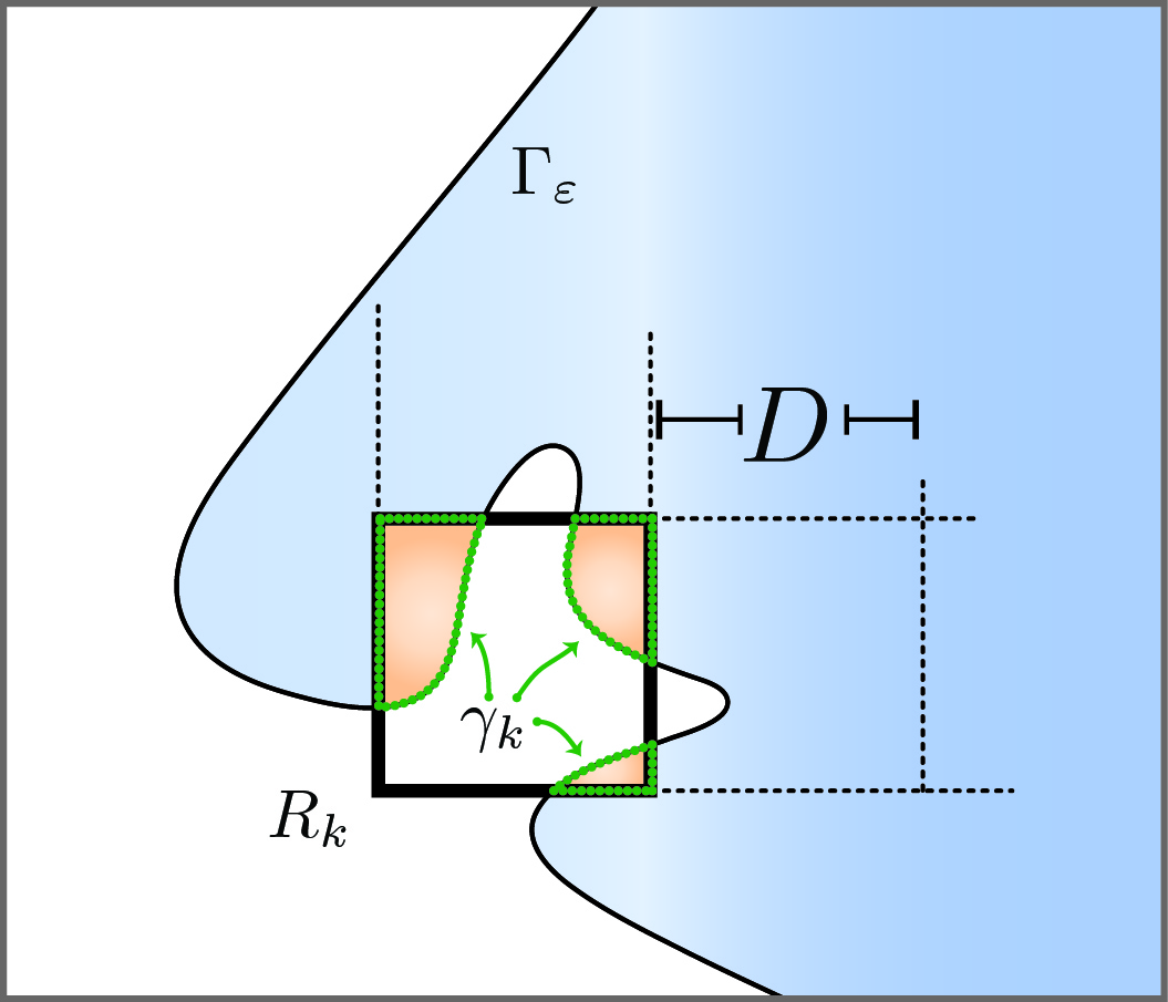
Figure 6: Aspects described in the proof of Lemma 4.4.

Claim. Let $z_{k}\in R_{k}$ (if $R_{k}$ intersects $\partial\Lambda_{\varepsilon}$ then choose $z_{k}$ in accordance with item (i) of the definition of $\sigma$–holomorphicity so that Hölder continuity of $Q$ can be assumed). Then

$$\oint_{\gamma_{k}}q\cdot Q~{}dz=q(z_{k})\cdot\oint_{\gamma_{k}}Q~{}dz+\mathcal{E}_{k},$$ (4.2)

where

$$|\mathcal{E}_{k}|\lesssim|\gamma_{k}|\cdot\|q\|_{C^{1}}\cdot D^{1+\sigma}$$

and to avoid clutter, we omit the $\varepsilon$ subscript on the $Q$’s.

Proof of Claim. Let us write

$$Q(z)=Q(z_{k})+\delta Q(z)$$

and similarly,

$$q(z)=q(z_{k})+\delta q(z).$$

We then have that

$$\oint_{\gamma_{k}}q\cdot Q~{}dz-q(z_{k})\cdot\oint_{\gamma_{k}}Q~{}dz=\oint_{\gamma_{k}}\delta Q\cdot\delta q~{}dz+Q(z_{k})\cdot\oint_{\gamma_{k}}\delta q~{}dz.$$

The second term on the right hand side vanishes identically by analyticity of $q$ whereas the integrand of the first term, by the assumed Hölder continuity of $Q$ and analyticity of $q$, can be estimated via $\lesssim$ $\|q\|_{C^{1}}\cdot D\cdot D^{\sigma}$ and the claim follows. ∎

Therefore we may write

$$\oint_{\Gamma_{\varepsilon}}q\cdot Q~{}dz=\sum_{k}\oint_{\gamma_{k}}q\cdot Q~{}dz:=\sum_{k}q(z_{k})\cdot\oint_{\gamma_{k}}Q~{}dz+\sum_{k}\mathcal{E}_{k},$$

where $z_{k}$ is a representative point in the region $R_{k}\cap\mbox{Int}(\Gamma_{\varepsilon})$. We divide the error on the righthand side into two terms, corresponding to interior boxes – which do not intersect $\Gamma_{\varepsilon}$, and boundary boxes – the complementary set.

Let us first estimate the interior boxes. Here, from the claim we have that the integral over each such box incurs an error of $\|q\|_{C^{1}}\cdot D^{2+\sigma}$ since here $|\gamma_{k}|\lesssim D$. There are of the order $|{\rm{Int}}(\Gamma_{\varepsilon})|\cdot D^{-2}$ interior boxes so we arrive at the estimate $\|q\|_{C^{1}}\cdot D^{\sigma}\cdot|{\rm{Int}}(\Gamma_{\varepsilon})|$. On the other hand, for boundary boxes, the contribution to the errors from the boundary boxes will certainly contain the original contour length $|\Gamma_{\varepsilon}|$. To this we must add $\lesssim$ $D$ $\times$ [the number of boundary boxes] corresponding to the “new” boundary of the boxes themselves that we might have introduced by considering the boxes in the first place. This is estimated as follows:

Claim. Let $M(\Gamma_{\varepsilon},D)$ denote the number of boundary boxes – i.e., the number of boxes on the grid visited by $\Gamma_{\varepsilon}$. Then $M\lesssim|\Gamma_{\varepsilon}|/D$.

Proof of claim. Since arguments of this sort have appeared in the literature (e.g., [8], [9]) many times, we shall be succinct: we divide the grid into 9 disjoint sublattices each of which is indicated by its position on a $3\times 3$ square. Let $M_{1},\dots,M_{9}$ denote the number of boxes of each type that are visited by $\Gamma_{\varepsilon}$. We may assume without loss of generality that $\forall j$, $M_{1}\geq M_{j}$. Let us consider the coarse grained version of $\Gamma_{\varepsilon}$ as a sequence of boxes on the first lattice (visited by $\Gamma_{\varepsilon}$); revisits of a given box are not recorded until/unless a different element of the sublattice has been visited in–between. Since the distance between each visited box is more than $D$ it follows that corresponding to each visited box the curve $\Gamma_{\varepsilon}$ must “expend” at least $D$ of its length, i.e., $|\Gamma_{\varepsilon}|\cdot D\geq M_{1}\geq(1/9)\cdot M$ and the claim follows. ∎

It is specifically observed that the additional boundary length incurred is at most comparable to the original boundary length. In any case altogether we acquire an estimate of the order $|\Gamma_{\varepsilon}|\cdot\|q\|_{C^{1}}\cdot D^{1+\sigma}$. We have established

$$|\sum_{k}\mathcal{E}_{k}|\lesssim\|q\|_{C^{1}}\cdot D^{\sigma}\cdot(|{\rm{Int}}(\Gamma_{\varepsilon})|+|\Gamma_{\varepsilon}|\cdot D).$$

Finally, by item ii) of ($\sigma,\rho$)–holomorphicity,

$$\sum_{k}|q(z_{k})\cdot\oint_{\gamma_{k}}Q~{}dz|\lesssim\|q\|_{\infty}\cdot\varepsilon^{\rho}\cdot(|{\rm{Int}}(\Gamma_{\varepsilon})|\cdot D^{-1}+|\Gamma_{\varepsilon}|).$$

This follows from the decomposition similar to the estimation of the $\mathcal{E}_{k}$ terms with the first term corresponding to interior boxes and the second to boundary boxes. The lemma been established. ∎

We can now immediately control the Cauchy integral of a $(\sigma,\rho)$–holomorphic function uniformly away from the boundary:

Corollary 4.5

Let $Q_{\varepsilon}$ be part of a $(\sigma,\rho)$–holomorphic sequence as described in Definition 4.1 above. Let $G_{\varepsilon}(z)$ be given as the Cauchy–integral of $Q_{\varepsilon}$ – as in Eq.(4.4) – over some (discrete Jordan) contour $\Gamma_{\varepsilon}$. Let $z$ denote any lattice point in ${\rm Int}(\Gamma_{\varepsilon})$ such that

$${\rm dist}(z,\Gamma_{\varepsilon})\geq n^{-a_{5}}:=d_{1}$$

for some $a_{5}>0$ and let $D\gg\varepsilon$ (both considered small). Then for all $\varepsilon>0$ sufficiently small, and any $d_{2}<d_{1}$,

$$\begin{split}|G_{\varepsilon}(z)-Q_{\varepsilon}(z)|&=|\frac{1}{2\pi i}\oint_{\Gamma_{\varepsilon}}(Q_{\varepsilon}(\zeta)-Q_{\varepsilon}(z))\cdot\frac{1}{\zeta-z}~{}d\zeta~{}|\\ &\lesssim\left(\frac{\varepsilon^{\rho}}{d_{2}D}+\frac{D^{\sigma}}{d_{2}^{2}}\right)\cdot(|{{\rm{Int}}}(\Gamma_{\varepsilon})|+|\Gamma_{\varepsilon}|\cdot D)+\left(\frac{d_{2}}{d_{1}}\right)^{\sigma}\end{split}$$ (4.3)

Proof.

This is the adaptation of standard arguments from the elementary theory of analytic functions to the present circumstances. Let $\gamma_{d_{2}}$ denote an approximately circular contour that is of radius $d_{2}$ and which is centered at the point $z$. Let $\Gamma_{\varepsilon}^{\prime}$ denote the contour $\Gamma_{\varepsilon}$ together with $\gamma_{d_{2}}$ – traversed backwards – and a back and forth traverse connecting the two. We have, by Lemma 4.4, that

$$|\frac{1}{2\pi i}\oint_{\Gamma_{\varepsilon}^{\prime}}(Q_{\varepsilon}(\zeta))\cdot\frac{1}{\zeta-z}~{}d\zeta~{}|\lesssim\left(\frac{\varepsilon^{\rho}}{d_{2}D}+\frac{D^{\sigma}}{d_{2}^{2}}\right)\cdot(|{{\rm{Int}}}(\Gamma_{\varepsilon})|+|\Gamma_{\varepsilon}|\cdot D)$$

where, in the language of this lemma, we have used $\|q\|_{\infty}\lesssim d^{-1}_{2}$ and $\|q\|_{C^{1}}\lesssim d^{-2}_{2}$. Thus we write

$$G_{\varepsilon}(z)=\frac{1}{2\pi i}\oint_{\gamma_{d_{2}}}\frac{Q_{\varepsilon}(\zeta)}{\zeta-z}d\zeta+\mathcal{E}_{2},$$

with $|\mathcal{E}_{2}|$ bounded by the right hand side of the penultimate display. So, subtracting $Q_{\varepsilon}(z)$ in the form

$$Q_{\varepsilon}(z)=\frac{1}{2\pi i}\oint_{\gamma_{d_{2}}}\frac{Q_{\varepsilon}(z)}{\zeta-z}d\zeta,$$

we have that

$$|G_{\varepsilon}(z)-Q_{\varepsilon}(z)|\lesssim|\mathcal{E}_{2}|+\frac{1}{2\pi}\oint_{\gamma_{d_{2}}}\frac{|Q_{\varepsilon}(z)-Q_{\varepsilon}(\zeta)|}{\zeta-z}d\zeta$$

and the stated result follows immediately from the Hölder continuity of $Q_{\varepsilon}$. ∎

By inputing information on $|\partial\Omega_{n}^{\square}|$, the required Cauchy–integral estimate now follows:

Proof of Lemma 3.5. We first recall the statement of the lemma:

Let $\Omega_{n}^{\square}$ and $S_{n}^{\square}$ be as in Proposition 3.2 so that

$$|\partial\Omega_{n}^{\square}|\leq n^{\alpha(1-a_{1})},$$

where $M(\partial\Omega)<1+\alpha$. For $z\in\Omega_{n}^{\square}$ (with the latter regarded as a continuum subdomain of the plane) let

$$F_{n}^{\square}(z)=\frac{1}{2\pi i}\oint_{\partial\Omega_{n}^{\square}}\frac{S_{n}^{\square}(\zeta)}{\zeta-z}~{}d\zeta.$$ (4.4)

Then for $a_{1}$ sufficiently close to 1 there exists $0<\beta<\sigma,\rho$ and some $a_{5}>0$ such that for all $z\in\Omega_{n}^{\square}$ so that $\mbox{dist}(z,\partial\Omega_{n}^{\square})>n^{-a_{5}}$,

$$\left|S_{n}^{\square}(z)-F_{n}^{\square}(z)\right|\lesssim n^{-\beta}.$$

By Proposition 4.3, we have that the functions $S_{n}^{\square}(z)$ (with $\varepsilon=n^{-1}$) have the $(\sigma,\rho)$–holomorphic property. In addition, we shall also have to keep track of a few other powers of $\varepsilon$, which we now enumerate:

1. let us define $b_{1}>0$ so that in macroscopic units we have

   $$|\partial\Omega_{N}^{\square}|\leq\varepsilon^{-\alpha(1-a_{1})}:=\varepsilon^{-\alpha b_{1}};$$

2. let us define

   $$d_{2}:=\varepsilon^{s},$$

   for some $s>0$ to be specified later;

3. finally, we define

   $$D:=\varepsilon^{t},$$

   where the role of $D$ will be the same as in the proof of Lemma 4.4 (it is the size of a renormalized block).

Plugging into Corollary 4.5 (again with $n^{-a_{5}}=d_{1}$) we obtain that

$$\begin{split}\left|S_{n}^{\square}(z)-F_{n}^{\square}(z)\right|&\lesssim\left(\frac{\varepsilon^{\rho}}{d_{2}D}+\frac{D^{\sigma}}{d_{2}^{2}}\right)\cdot(|{{\rm{Int}}}(\partial\Omega_{n}^{\square})|+|\partial\Omega_{n}^{\square}|\cdot D)+\left(\frac{d_{2}}{d_{1}}\right)^{\sigma}\\ &\lesssim\left(\varepsilon^{\rho-(s+t)}+\varepsilon^{t\sigma-2s}\right)\cdot(1+\varepsilon^{-\alpha b_{1}+t})+\frac{\varepsilon^{s\sigma}}{d_{1}^{\sigma}}\\ &=\varepsilon^{\rho-(s+t)}+\varepsilon^{\rho-s-\alpha b_{1}}+\varepsilon^{t\sigma-2s}+\varepsilon^{(1+\sigma)t-\alpha b_{1}-2s}+\frac{\varepsilon^{s\sigma}}{d_{1}^{\sigma}}.\end{split}$$

With $\sigma$ fixed, the parameters $s,t>0$ and $d_{1}$ can be chosen so that all terms in the above are positive powers of $\varepsilon$: set $t=\lambda\sigma$, where $\lambda\in(0,1)$ so that $\sigma>\frac{1-\lambda}{\lambda}$. This choice of $t$ implies that $(1+\sigma)t>\sigma>t$. Now let $s>0$ and $b_{1}>0$ be sufficiently small so that $2s<t\sigma$ and $\alpha b_{1}<t$ so altogether we have the last two terms are positive powers of $\varepsilon$. Next take $t$ and then $s$ and $b_{1}$ even smaller if necessary, we can also ensure that $\rho>s+t$ and $\rho>s+\alpha b_{1}$. Finally, $d_{1}$ can be chosen to be some power of $\varepsilon$ so that $\varepsilon^{s}\ll d_{1}$.

∎

5 Harris Systems

This last section is devoted to the proof of Theorem 3.10, although the construction may be of independent interest and find further utility.

5.1 Introductory remarks

For many purposes, the pertinent notion of distance – or separation – is Euclidean; in the context of critical percolation, what is more often relevant is the logarithmic notion of distance: how many scales separate two points. These matters are relatively simple deep in the interior of a domain or in the presence of smooth boundaries. However, for points in the vicinity of rough boundaries, circumstances may become complicated. For certain continuum problems, including, in some sense, the limiting behavior of critical percolation, there is a natural notion for a system of increasing neighborhoods about a boundary point: the preimages under uniformization of the logarithmic sequence of cross cuts centered about the preimage of the boundary point in question. This device was employed implicitly and explicitly at several points in [5]. In the present context, we cannot so easily access the limiting behavior we are approaching. Moreover, in order to construct such a neighborhood sequence at the discrete level, it will be necessary to work directly with $\Omega_{n}$ itself.

We will construct a neighborhood system for each point in $\partial\Omega_{n}$ by inductively exploring the entire domain via a sequence of crossing questions. Our construction demonstrates (as is a posteriori clear from the convergence of $S_{n}$ to a conformal map) that various domain irregularities e.g., nested tunnels, which map to a small region under uniformization are, in a well–quantified way, also unimportant as far as percolation is concerned.

5.2 Preliminary Considerations

For completeness let us first recall the setting. Let $\Omega\subset\mathbb{C}$ be a simply connected domain with $\text{diam}(\Omega)<\infty$ and let $2\Delta$ denote the supremum of the radius of all circles which are contained in $\Omega$. Further, let $\mathcal{D}_{\Delta}$ denote a circle of radius $\Delta$ with the same center as a circle for which the supremum is realized. We will denote by $\Omega_{m}$ any interior discretization of $\Omega$, e.g., one of the types discussed before; we use $n^{-1}$ to denote the lattice spacing. For $\omega\in\partial\Omega_{m}$ we will define a sequence of segments the boundaries of which are paths beginning and ending on $\partial\Omega_{m}$. As a rule, these segments separate $\omega$ from $\mathcal{D}_{\Delta}$. The dimensions of these segments will be determined by percolation crossing probabilities analogous to the system of annuli (of which these are fragments) investigated by Harris in [11]. Notwithstanding that the regions between segments do not actually form annuli, we will refer to the resultant objects as Harris rings – or, occasionally, ring segments, annular fragments, etc. The ultimate goal will be to ensure that Harris rings have uniform upper and, to some extent, lower bounds on their crossing probabilities (among other properties). Moreover, these represent the essence of what must be traversed by paths emanating from $\mathcal{D}_{\Delta}$ which reach to “the essential vicinity” of the point $\omega$. Details will unfold with the construction. The ultimate object will be called the Harris system stationed at $\omega$.

We will start with the preliminary considerations of the construction. Let $S_{0}(\omega)$ denote the smallest square (i.e., lattice approximation thereof) which is centered at $\omega\in\partial\Omega_{m}$ and whose boundary intersects $\mathcal{D}_{\Delta}$. That is to say, the boundary is approximately tangent to $\partial\mathcal{D}_{\Delta}$. We set $R_{0}(\omega):=S_{0}(\omega)\cap\Omega_{m}$. Successive topological rectangles $A_{1}(\omega),\dots,A_{k}(\omega),\dots$ which may be envisioned as the intersection of $\Omega_{m}$ with a nested sequence of square annuli centered at $\omega$ will in practice be constructed via a non–trivial inductive procedure: 1) there will be deformations of the shape of the annular segments; 2) the sizes of the “smaller squares” (i.e., the location of the “next” boundary) will be determined by percolation crossing probabilities; 3) the basic shape will not always be a square centered at $\omega$. Nevertheless, we will call these annular (ring) fragments.

The annular fragment $A_{k}$ will have four boundary pieces, forming a topological rectangle; opposing pairs of boundaries will be denoted as yellow and blue with blue corresponding to a portion of $\partial\Omega_{m}$. The rectangle $A_{k}$ will constitute an arena for exclusive crossing type events e.g., yellow crossings between the yellow boundaries and blue crossings between the blues. A good portion of our inductive procedure involves the refinement and coloring of the boundaries.

All points on the yellow boundaries can be connected to $\omega$ via a (self–avoiding) path in the complement of $\partial\Omega_{m}$ and in the complement of the blue boundaries. The outer and inner yellow boundaries may be – somewhat loosely – defined by the stipulation that all such paths to the outer boundary must first pass through the inner boundary. Already, it is the case that all of $\partial\Omega_{m}\cap\partial A_{k}$ is blue; indeed, envisioning $A_{k}$ as the intersection of $\Omega_{m}$ with an actual square annulus, some of the blue boundary will be where $\partial\Omega_{m}$ cuts through such a ring.

Key in the initial portion of the construction is that for some $\vartheta$ with $0<\vartheta<1/2$, it will be the case that the probability of a yellow crossing between the yellow segments of the boundaries and the probability of a blue crossing between the blue segments of the boundaries are both in excess of $\vartheta$ (and therefore less than $1-\vartheta$). Eventually we will forsake the lower bound for the yellow crossings in favor of an ostensibly much smaller bound pertaining to geometric properties of the annular fragments which permit yellow crossings under tightly controlled conditions. And, eventually, we may have to consider $\vartheta$ as a small parameter. Nonetheless all quantities will be uniform in the ultimate progression of fragments and in the lattice spacing $n^{-1}$ for $n$ sufficiently large.

The essence of the geometric property which we will require of the Harris regularization scheme is that $\omega$ – or its relevant vicinity – can be connected to $\mathcal{D}_{\Delta}$ via a sequence of boxes housed within the ring fragments. The size of the boxes is uniform within a layer and does not increase or decrease too fast between neighboring layers. While the box sizes may be “small”, this will only be relative to the characteristic scale of the layer via a numerical constant which is independent of $n$ and the particulars of the fragment. Thus, the scale of the boxes may be considered comparable to the scale of the fragments to which they belong.

Dually, $\omega$ can be “sealed off” from $\mathcal{D}_{\Delta}$ by the independent events of separating paths which have an approximately uniform probability in each segment. Thus we envision an orientation to our constructions leading from $\mathcal{D}_{\Delta}$ to $\omega$. (Indeed, it is this orientation which permits us to choose the appropriate components to be colored yellow at various stages of the construction.) Moreover, from these considerations, it emerges that only the first $O(\log n)$ of these segments are relevant for the problems under consideration. If $\Omega_{m}$ has a smooth boundary this would, in fact, be all of them; under general circumstances, as it turns out, the configurations in the region beyond the first $O(\log n)$ segments have negligible impact on the percolation problem at hand.

We will describe what is fully required in successive stages of increasing complexity, but before we begin, let us dispense with some geometric and some lattice details. While the definitions and conventions which follow are certainly not all immediately necessary – and possibly unnecessary for an understanding of the overall scheme – we have elected to display them at the outset in a place where they are readily accessible. The reader is invited to skim these lightly and later, if required, refer back to these paragraphs.

Preliminary definitions. The moral behind the upcoming definitions is that all lattice details should be resolved in as organic a way as possible via the definition of the percolation properties for the model at hand. All of the models of interest for us have representations which are hexagonal based: each model provides some smallest independent unit (abbreviated SIU) in the sense that such a unit (a subset of the lattice) can be stochastically configured independently of one another and any smaller subset is either empty or is correlated with some neighbor. In the case of independent hexagonal tiling, the smallest such unit is simply a hexagon whereas for the generalized models in [10] the smallest unit can be either a single hexagon or a flower (which consists of 7 hexagons). All notions of neighborhood, self–avoiding, etc., are now to be thought of in terms of the intrinsic definition of connectivity associated with the underlying percolation problem. However, it is pointed out that in the case of the models introduced in [10], path transmissions may take place over fractions of hexagons.

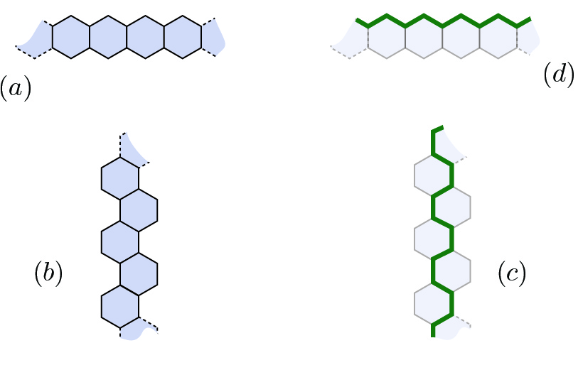
Figure 7: Various of notions of horizontal and vertical consistent with hexagonal tiling: $(a)$ a horizontal string $(b)$ a vertical string $(c)$ a vertical segment $(d)$ a horizontal segment.

1. A string of hexagons is a sequence of hexagons with no repeats each of which – save the first – has an edge in common with its predecessor. Similarly, a segment is a self–avoiding path consisting of edges (which are the boundary elements of hexagons). With apology, both objects will on occasion be referred to as paths; in all cases, the relevant notion will be clear from context and/or the distinction will be of no essential consequence. Similarly, if $\mathcal{A}\subset\Omega_{m}$ is a connected set of hexagons then the boundary, $\partial\mathcal{A}$, could mean the hexagons in $\overline{\Omega}_{m}\setminus\mathcal{A}$ which share an edge with an element of $\mathcal{A}$ or the segment consisting of the afore described shared edges. Again, the distinction will usually be unimportant but, if need arises will be made explicit.

2. For $x,y\in\overline{\Omega}_{m}$, we will use $\mathscr{P}:x\leadsto y$ to denote a string in $\Omega_{m}$ connecting $x$ and $y$. By contrast, the event $\{x\leadsto y\}$ will mean, in the pure hexagon problem, the existence of a $\mathscr{P}:x\leadsto y$ such that each element of $\mathscr{P}$ is of the same color thereby forming a monochrome percolation connection (or transmission) between these points. For the more general cases, $\{x\leadsto y\}$ also denotes this monochrome connectivity event but here some of the transmissions may take place through hexagon fragments (see, if desired, [10], Figure 1).

3. We shall often use descriptions like horizontal and vertical, and this should be understood to mean the closest lattice approximation to either a horizontal or vertical segment. The precise details are actually unimportant but recall that, to be definitive, we have assumed that hexagons are oriented so that there are two vertical edges parallel to the $y$–axis. For the moment, let us discuss the pure hexagon problem.

   A horizontal string of hexagons would consist of a sequence of neighboring hexagons the centers of which are horizontally aligned. Thus, each hexagon in the string shares only vertical edges in common with its neighbors or neighbor. By contrast, a vertical string of hexagons will “zigzag” a bit. E.g., the $k^{\text{th}}$ hexagon in the sequence shares in common the segments to the left of the right vertical segment with the $(k\pm 1)^{\text{st}}$ hexagon. And similarly for the $(k+2)^{\text{nd}}$ hexagon in the sequence. More pertinently, a horizontal segment consists, e.g., of the tops of hexagons in a horizontal string with each hexagon in the string contributing (except, perhaps at the endpoints) the two edges above and adjacent to the vertical. A vertical segment alternates e.g., between left vertical edges on even hexagons and, for the odd hexagons, the entire left sides connect these (even vertical edges) together. Thus, horizontal segments are above or below horizontal strings and similarly vertical segments are to the left or right of vertical strings. See figure 7. Square boxes will be understood as already aligned with respect to the fixed Cartesian axes with boundaries consisting of vertical and horizontal segments as described.

   There is a natural notion of neighboring segments, namely with a fixed string in mind, the segment which is of (approximately) the same length that is on the other side of the string. More formally, given a segment and associated string, the next segment in the direction of the string is given by the symmetric difference over all hexagons in the string of the edges of each hexagon and then deleting the initial segment. These observations will be useful when we define the concept of sliding. Notwithstanding, the ends of strings and segments must often be tended to on an individual basis as is the case of composite SIU.

   For extended SIU – flowers – for now it is only important to state a few rules: for strings, the entire SIU must be incorporated as a single unit. It should be noted that this incorporation can have a variety of manifestations; e.g., in the case of horizontal segments, there are three levels at which the string may impinge. However, all pure hexagons in a horizontal string must still have their centers horizontally aligned. Similarly for the case of vertical strings. In conjunction with the above, segments are forbidden to pass through the flower and therefore must circumvent. In the context of extended SIU, there will be some small amount of “special considerations” when we turn our discussion to distances and neighborhoods.

4. If If $x=(x_{1},x_{2})$ and $y=(y_{1},y_{2})$ are SIU in $\Omega_{m}$ and $V\subseteq\Omega_{m}$ then we define the distance $d_{\infty}^{V}(x,y)$ to be the $L^{\infty}$– distance, i.e., $\max\{|x_{1}-x_{2}|,|y_{1}-y_{2}|\}$, subject to the local connectivity constraint that they can actually be connected within the stated distance scale. With precision: if $b_{L}$ is notation for a box of side–length $2L$ then

   $$d_{\infty}^{V}(x,y)=\min\{L\mid\exists b_{L}\text{ such that a string in $b_{L}$ contains $x$ and $y$}\}.$$

   If no such $b_{L}$ exists – i.e., if it is not the case that both $x$ and $y$ are in $V$, than we will regard $d_{\infty}^{V}(x,y)$ as being infinite.

   If $\mathscr{X}$ and $\mathscr{Y}$ are sets in $V$, then $d_{\infty}^{V}(\mathscr{X},\mathscr{Y})$ is defined in the usual way, i.e.,

   $$d_{\infty}^{V}(\mathscr{X},\mathscr{Y})=\inf_{x\in\mathscr{X},y\in\mathscr{Y}}~{}d_{\infty}^{V}(x,y).$$

   Once again, with apology, we will also use $d_{\infty}^{(\cdot)}(\cdot)$ to denote similar minded distances between pairs (or sets) of edges and, often enough, omit the superscript when it is clear from context.

5. Similar to the above item: let $\Gamma$ denote a segment or a string. Then $\|\Gamma\|_{\infty}$ denotes the $d_{\infty}^{\Gamma}$– or $L^{\infty}$– diameter of $\Gamma$.

6. A topological rectangle is a simply connected subset of $\Omega_{m}$ containing all its SIU that has four marked points on the boundary dividing the boundary into two pairs of “opposing” segments: $(\mathscr{L},\mathscr{R})$ and $(\mathscr{T},\mathscr{B})$. We envision such a rectangle as a stadium for a dual percolation crossing problem.

Definition 5.1 (Sliding).

Let $q$, $q^{\prime}$ denote points in $\overline{\Omega}_{m}$. Let $z_{1},z_{2}\in\partial\Omega_{m}$ and let $\Gamma$ denote a segment in $\Omega_{m}$, connecting $z_{1}$ to $z_{2}$ and which separates $q$ and $q^{\prime}$. Thus, $\Omega_{m}$ is disjointly decomposed into the connected components $\mathscr{C}_{\Gamma}(q)$ and $\mathscr{C}_{\Gamma}(q^{\prime})$ of $q$ and $q^{\prime}$ respectively with the sets $\mathscr{C}_{\Gamma}(q)$ and $\mathscr{C}_{\Gamma}(q^{\prime})$ having $\Gamma$ as a common portion of their boundaries. If necessary, it is assumed that $\Gamma$ is such that $\mathscr{C}_{\Gamma}(q)$ – and hence $\mathscr{C}_{\Gamma}(q^{\prime})$ do not contain any partial SIU. Moreover, to avoid spurious complications, it is assumed that the $L^{\infty}$ separation between $\Gamma$ and $q^{\prime}$ is at least a few units in excess of the $\ell$ to be discussed below.

We now define the sliding of $\Gamma$ by $\ell$ units in the direction of $q^{\prime}$. In essence, this is the construction of a new segment – which we denote by $\Gamma^{\prime}$ – that is $\ell$ units closer to $q^{\prime}$ and, correspondingly $\ell$ units further from $q$. The segment $\Gamma^{\prime}$ also connects some $z_{1}^{\prime}$ and $z_{2}^{\prime}$ on $\partial\Omega_{m}$ and, most importantly, also separates $q$ from $q^{\prime}$. The segment $\Gamma^{\prime}$ in most cases can be envisioned as a displacement of $\Gamma$ with some natural adjustments. We reiterate that, as was the case above, the microscopic details are not essential and may be omitted in a preliminary reading.

Let $\mathbf{h}_{\Gamma,q}$ denote the hexagons in $\mathscr{C}_{\Gamma}(q)$ which have at least one edge in $\Gamma$ and for $h\in\mathbf{h}_{\Gamma,q}$, let $N_{\ell,\mathscr{C}(q^{\prime})}(h)$ denote the radius $\ell$ neighborhood of $h$ using the $d_{\infty}^{\mathscr{C}_{\Gamma}(q^{\prime})}$– distance:

$$N_{\ell,\mathscr{C}_{\Gamma}(q^{\prime})}(h)=\{h^{\prime}\mid d_{\infty}^{\mathscr{C}_{\Gamma}(q^{\prime})}(h,h^{\prime})\leq\ell\}.$$

Next we have

$$\tilde{N}_{\ell,\mathscr{C}_{\Gamma}(q^{\prime})}(\Gamma)=\underset{h\in\mathbf{h}_{\Gamma,q}}{\cup}N_{\ell,\mathscr{C}_{\Gamma}(q^{\prime})}(h)$$

this set along with the completion of any partial SIU it contains may be regarded as the relevant $k$–neighborhood of $\Gamma$ and will be denoted as above without the tilde. The “$\ell$–slide” of $\Gamma$ will be a subset of the edge boundary of $N_{\ell,\mathscr{C}_{\Gamma}(q^{\prime})}(\Gamma)$.

Indeed, let us consider

$$\tilde{\Gamma}^{\prime}=\partial N_{\ell,\mathscr{C}_{\Gamma}(q^{\prime})}(\Gamma)\setminus(\partial\Omega_{m}\cup\Gamma)$$

where in the above, both notions of boundary refer to edge boundaries. It is evident that $\tilde{\Gamma}^{\prime}$ consists of one or more segments each of which must begin and end on the domain boundary. Let us denote these segments by $\Gamma_{1}^{\prime},\Gamma_{2}^{\prime},\dots$; one of these will be selected as the new segment $\Gamma^{\prime}$.

We now claim that exactly one $\Gamma^{\prime}_{j}$ separates $q$ from $q^{\prime}$. Indeed let us reconsider the amalgamated $\tilde{\Gamma}^{\prime}$: since $q^{\prime}\notin\overline{N}_{\ell,\mathscr{C}_{\Gamma}(q^{\prime})}(\Gamma)$ (because of the assumed distance between $q^{\prime}$ and $\Gamma$ in excess of $\ell$) it is clear that $\tilde{\Gamma}^{\prime}$ separates $q^{\prime}$ from $\Gamma$ and hence certainly separates $q$ and $q^{\prime}$. Thus any self–avoiding path of edges $\Omega_{m}$ connecting $q$ and $q^{\prime}$ must intersect $\tilde{\Gamma}^{\prime}$ and the above claim is now readily established.

Indeed, consider the set $\mathscr{C}_{\Gamma}(q^{\prime})\setminus N_{\ell,\mathscr{C}_{\Gamma}(q^{\prime})}(\Gamma)$ which consists of connected components $K_{1}$, $K_{2}$, etc. The edge boundaries of these $K_{j}$’s consist of an edge segment of $\partial\Omega_{m}$ joined together with an edge segment from $\tilde{\Gamma}^{\prime}$ the latter of which correspond to the aforementioned $(\Gamma^{\prime}_{j})$’s. If $q^{\prime}\in\Omega_{m}$ then we observe that only one of these $K_{j}$ can contain it and this corresponds to the $\Gamma_{j}^{\prime}$ selected. If $q^{\prime}\in\partial\Omega_{m}$, then, similarly, only one of the $K_{j}$ uses edges of this hexagon (where we again invoke the fact that the separation between $q^{\prime}$ and $\Gamma$ is in excess of $\ell$) and this corresponds to the $\Gamma_{j}^{\prime}$ selected.

Let us use $A$ as notation for the connected region bounded by $\Gamma$, $\Gamma^{\prime}$ and the appropriate portion of $\partial\Omega_{m}$. Then it is noted that to within a few lattice spacings (due to inherent discreetness and the possible effects SIU) all points on $\Gamma^{\prime}$ are the same $d_{\infty}^{A}$– distance from $\Gamma$. However, it should be noted that due to the possibility of pockets that had been sealed off by the now discarded $\Gamma_{j}^{\prime}$ there might well be points in $A$ considerably further from $\Gamma$ than $\Gamma^{\prime}$. Moreover, the contrast between $\Gamma^{\prime\prime}$ and $\Gamma^{\prime}$ with the former constructed via an $(\ell+1)$–neighborhood slide will be regarded – by definition – as the (precursory) addition, modulo the aforementioned discreet irregularities, of a single layer to $A$.

5.3 Preliminary Constructions

Using the above described sliding procedure, we will start with some initial segment which separates $\omega$ from $\mathcal{D}_{\Delta}$ (or some representative point therein) and consider the sequence of slides indexed by $\ell$ in the direction of $\omega$. We stop this procedure when certain criteria are satisfied within the region (which is a topological rectangle) whose boundary consists of the initial segment, the current slide and the relevant portions of the boundary. This region will be referred to as a ring fragment and the criteria will pertain to crossing probabilities within and certain geometric properties of the region itself. When the requisite criteria are satisfied, we will refer to the current slide (or certain modifications thereof) as the successor segment of the initial segment. It is this successor segment which then plays the role of the “initial” segment when the next successor is to be defined.

We remark that the overall construction is somewhat intricate due to the modifications to which we have already alluded. Indeed, the full assemblage will actually require an inductive procedure. Our expository methodology is as follows: we will first describe the one–step procedure, i.e., constructing an acceptable successor segment from some given segment and then describe the full logical inductive procedure in a last subsubsection; further, the one–step procedure may in itself be complicated so we have therefore broken the construction into three stages which we will call the $S$–construction, the $Q$–construction and the $R$–construction. We will describe them in order as they require more and more detailed control on successive Harris segments. In all cases we will refer to the running (current) initial segment as $Y_{I}$ and the constructed successor segment as $Y_{F}^{(\cdot)}$ where $(\cdot)$ indexes the relevant modification. At each stage, we need not make any specific claim as to the nature of $Y_{I}$ however, it may be generally assumed that $Y_{I}$ is such that it already satisfies the criteria $(\cdot)$.

Finally, we remark that for simple domains e.g., convex domains or domains bounded only by straight line segments, the vast majority of the forthcoming is unnecessary: here we create successors as just described stopping when crossing probability within the region acquires a desired value (the simplified S–construction) – or when a fixed scale determined by the domain has been reached – and then divide the region into boxes the scale of the region itself (the simplified R–construction). All of the up and coming technology concerns the possibility of (multi–scale) fjords, needle–like tunnel structures (on multi–scales) and similar minded impediments.

5.3.1 The $S$–Construction (Harris ring fragments)

The initial stage is the $S$–construction, which starts with a square centered at the specified $\omega\in\partial\Omega_{m}$. Recall the square $S_{0}(\omega)$ centered about $\omega$ and note that since $\partial\Omega_{m}\cap\partial\mathcal{D}_{\Delta}=\emptyset$ whereas $\partial\mathcal{D}_{\Delta}$ has non–trivial intersection with $\partial S_{0}(\omega)$, we can declare the first yellow segment of the boundary of the first ring fragment to be, simply, the connected component of $\partial S_{0}(\omega)\cap\partial\mathcal{D}_{\Delta}$ in $\Omega_{m}$. We denote this yellow boundary portion by $Y_{0}$.

Consider a a slide of $Y_{0}$ which we temporarily denote $\mathbb{X}_{S}$ and let $S=\mathscr{C}_{\mathbb{X}_{S}}(\omega)$. For immediate use and for future reference, let us define some auxiliary objects:

(a)   Let $\mathbf{P}_{\omega}$ be the set of all paths $\mathscr{P}:\omega\leadsto Y_{0}$ defined as usual: they are self–avoiding paths (strings) consisting of hexagons with $\mathscr{P}\subseteq\Omega_{m}\cup\{\omega\}$, and $\mathscr{P}\cap\partial\Omega_{m}=\{\omega\}$.

(b)   Let $\mathbb{Y}_{S}\subseteq\mathbb{X}_{S}$ be such that any $z\in\mathbb{Y}_{S}$ is the last point in $S$ for some $\mathscr{P}\in\mathbf{P}_{\omega}$. Note that in general these could be SIUs.

(c)   Let $Y_{S}\subset\mathbb{Y}_{S}$ be the set of points (edges) in $\mathbb{Y}_{S}$ that can be reached from $\omega$ by a portion of a path $\mathscr{P}\in\mathbf{P}_{\omega}$ which lies in the complement of $\mathbb{Y}_{S}$.

In general a string $\mathscr{P}$ may be regarded as a sequence of neighboring hexagons, a sequence of centers of neighboring hexagons (points of the original triangular lattice) connected by straight line segments (bonds of the original triangular lattice) or the corresponding sequence of edges separating the elements of the hexagon description (bonds of the honeycomb lattice dual to the aforementioned bonds). To avoid excessive clutter, here and in the future, we will be non–specific about such matters when they are of no actual consequence to the main argument. Some illustrations which indicate generic differences between the sets $Y_{S}$ and $\mathbb{Y}_{S}$ can be found in the inserts of Figure 8.

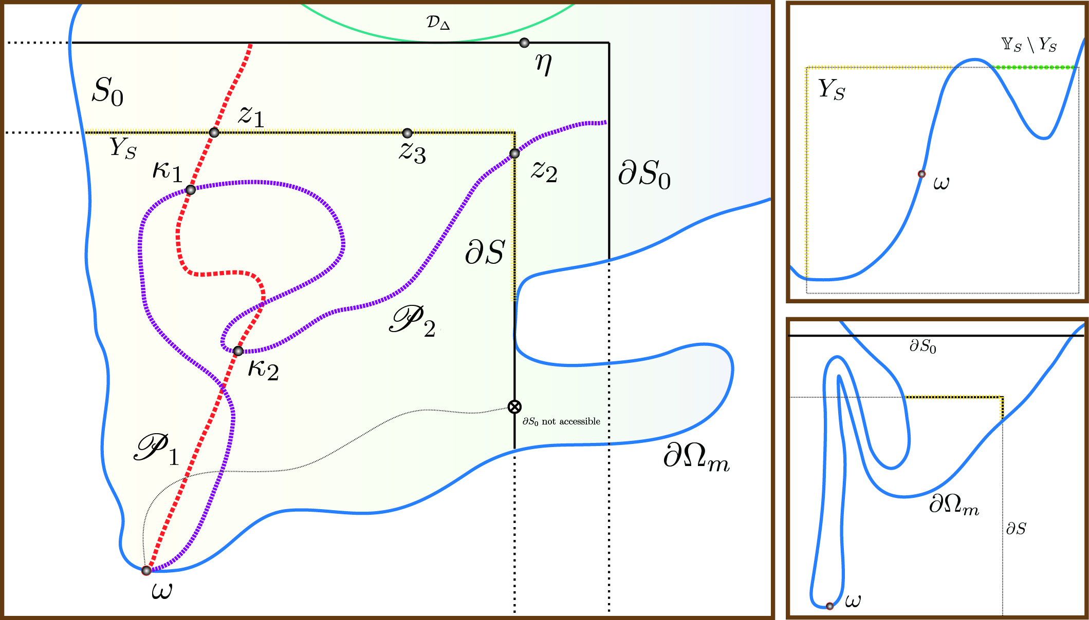
Figure 8: Illustration of the principal concepts for the proof that $Y_{S}$ is a connected set. In the example illustrated, the loop $\mathscr{L}$ is completed using portions of $\partial S_{0}$. Top insert: $\mathbb{Y}_{S}\neq Y_{S}$. Bottom insert: $\mathbb{Y}_{S}=Y_{S}$.

We shall refer to these $Y_{S}$ as yellow segments. We will now establish some elementary topological properties of these yellow segments $Y_{S}$; in particular, we claim that as segments, the $Y_{S}$ are in fact well–defined:

Claim. The set $Y_{S}$ as described above is non–empty and consists of a single connected component. Moreover, $Y_{S}$ separates $\omega$ from $Y_{0}$, i.e., every path in $\mathbf{P}_{\omega}$ contains at least one element of $Y_{S}$.

Proof of Claim. To establish that $Y_{S}$ is non–empty, let $\mathscr{P}\in\mathbf{P}_{\omega}$ and let $z\in\mathbb{Y}_{S}$ denote the first element of $\mathbb{Y}_{S}$ encountered by $\mathscr{P}$. Further, let $\mathscr{P}_{\text{I}}$ denote the (initial) portion of $\mathscr{P}$ till it reaches $z$. Now, by definition of the set there is some other $\mathscr{P}^{\prime}\in\mathbf{P}_{\omega}$ (which is possibly the same as $\mathscr{P}$) such that $z$ is the last element of $\mathscr{P}^{\prime}$ which is in $S$. We denote by $\mathscr{P}_{\text{F}}^{\prime}$ the (final) portion of $\mathscr{P}^{\prime}$ after it has passed through $z$. Now consider the path $\mathscr{R}$ which may be informally described as $\mathscr{P}_{\text{I}}\cup\{z\}\cup\mathscr{P}_{\text{F}}^{\prime}$. It is seen that $\mathscr{R}$ satisfies the requisite properties of a path described in item $($c) above for the point $z$ and so, indeed, $Y_{S}$ is not empty.

An argument along these lines also demonstrates that $Y_{S}$ separates $\omega$ from $Y_{0}$: again letting $\mathscr{P}\in\mathbf{P}_{\omega}$, we can consider $z$ as above. The same argument then shows that $z\in Y_{S}$ and thus we conclude that every path in $\mathbf{P}_{\omega}$ contains an element of $Y_{S}$.

We now turn to the central portion of the claim, namely that $Y_{S}$ is a single component. To this end, let us consider the ancillary paths which are along the lines of $\mathscr{R}$ above. This set of paths will be called $\mathbf{P}_{S}$ and each $\mathscr{P}\in\mathbf{P}_{S}$ has the property that it has a unique encounter with $\mathbb{Y}_{S}$ – which is necessarily a single element $z$ in $Y_{S}$. So, in particular, each $\mathscr{P}\in\mathbf{P}_{S}$ divides into a $\mathscr{P}_{\text{I}}$ – before the encounter with $Y_{S}$, a $\mathscr{P}_{\text{F}}$ – after the encounter with $Y_{S}$, and a point $z$ in $Y_{S}$ itself.

Foremost, it is clear by construction of paths along the lines of $\mathscr{R}$ that any $z\in Y_{S}$ has a $\mathscr{P}\in\mathbf{P}_{S}$ which goes through $z$. We further define $V_{S}$ to be the connected component of $\omega$ relative to the $\mathscr{P}_{\text{I}}$’s just described:

$$V_{S}=\{v\in\Omega_{m}\mid v\in\mathscr{P}_{\text{I}}\text{ for some }\mathscr{P}_{\text{I}}\subset\mathscr{P}\in\mathbf{P}_{S}\}$$

Similarly, we define $U_{S}$ to be the points reachable by some $\mathscr{P}_{\text{F}}\subset\mathscr{P}\in\mathbf{P}_{S}$. Formally, we define both sets as disjoint from $Y_{S}$ and adjoin $\omega$ to $V_{S}$.

Now it is noted that $\partial\Omega_{m}$ may in general divide $\partial S$ into many components so we are showing that only one of these contains $Y_{S}$. We refer the reader to Figure 8 for the up and coming argument. We must demonstrate that any $z_{1},z_{2}\in Y_{S}$ must be in the same component. We may as well assume that $z_{1}\neq z_{2}$ and that they are not neighbors, since otherwise it is immediate that they are in the same component.

Consider paths $\mathscr{P}_{1},\mathscr{P}_{2}$, in $\mathbf{P}_{S}$ which contain $z_{1}$ and $z_{2}$, respectively. The initial portions of these paths $\mathscr{P}_{\text{I},1}$ and $\mathscr{P}_{\text{I},2}$ may very well intersect, so let $\kappa_{1}$ denote the last such point along $\mathscr{P}_{\text{I},1}$ and similarly for $\kappa_{2}$; if there are no such point along the paths proper, then we define $\kappa_{1}=\kappa_{2}=\omega$. Nevertheless, we certainly allow the possibility that $\kappa_{1}=\kappa_{2}$. Assuming though that $\kappa_{1}\neq\kappa_{2}$, there is (for the sake of definitiveness) a portion of $\mathscr{P}_{\text{I},1}$ connecting $\kappa_{2}$ to $\kappa_{1}$ since, by definition, $\kappa_{1}$ was the last such “collision” point along $\mathscr{P}_{\text{I},1}$. Thus, starting at $z_{2}$, moving (backwards) along $\mathscr{P}_{2}$ till $\kappa_{2}$ is reached then moving (forwards) along $\mathscr{P}_{1}$ through $\kappa_{1}$ and on to $z_{1}$ we have achieved a path $z_{2}\leadsto z_{1}$ which is entirely in $V_{S}$. This latter path we regard as one part of a loop.

On the other side of $Y_{S}$, in $U_{S}$, we follow a similar procedure and define, in an analogous fashion, the points $\eta_{1}$ and $\eta_{2}$. Again, if no such points exist along the paths proper, then we join these paths together using the the relevant portion of $Y_{0}$. This constitutes another path $z_{1}\leadsto z_{2}$ which is disjoint from the first. This is the second part of the loop the entirety of which – including $z_{1}$ and $z_{2}$ – is denoted by $\mathscr{L}$. Now, with the possible exception of $\omega$ itself, $\mathscr{L}$ is disjoint from $\partial\Omega_{m}$. Thus, $\text{Int}(\mathscr{L})\subset\Omega_{m}$ and so the entire portion of $Y_{S}$ in between $z_{1}$ and $z_{2}$ lies within.

Let $z_{3}$ be one such point in between. Consider any path residing in $U_{S}$ from $z_{3}$ to the second half of the loop. (Such a path may be acquired by attempting a path $z_{3}\leadsto\partial S_{0}$ – in $U_{S}$ – until obstructed.) Joining this path with the relevant portions of, $\mathscr{P}_{\text{F},1}$ and/or $\mathscr{P}_{\text{F},2}$ we now have a path $z_{3}\leadsto\partial S_{0}$ in $U_{S}$. Performing a similar construction in $V_{S}$ we get a path $z_{3}\leadsto\omega$ in $V_{S}$ and putting these two together we have constructed a bona fide $\mathscr{P}_{3}\in\mathbf{P}_{S}$ which contains $z_{3}$. We have therefore demonstrated $z_{3}\in Y_{S}$ as desired. ∎

Next we may consider a further successor segment $Y_{S^{\prime}}$ of $Y_{S}$ and the corresponding component of $\omega$, $S^{\prime}$. Then we have the following “partial ordering” property:

Claim. Let $S$, $S^{\prime}$, $Y_{S^{\prime}}$ etc. be as described. Then $Y_{S}$ separates $Y_{S^{\prime}}$ from $Y_{0}$ and $Y_{S^{\prime}}$ separates $Y_{S}$ from $\omega$. A similar result holds for intermediate $Y$– segments. E.g., if $Y_{S^{\dagger}}$ is an earlier successor of $Y_{0}$ than $Y_{S}$, then $Y_{S^{\dagger}}$ separates $Y_{0}$ from $Y_{S}$ or if $Y_{S^{\dagger}}$ is an intermediate successor segment between $Y_{S^{\prime}}$ and $Y_{S}$, then $Y_{S^{\dagger}}$ separates $Y_{S}$ from $Y_{S^{\prime}}$ etc.

Proof of Claim. This follows readily from the ideas invoked in the proof of the previous claim. Consider $\mathscr{P}:Y_{S^{\prime}}\leadsto Y_{0}$ and define $\mathscr{P}_{\text{F},S^{\prime}}$ to be the portion of this path after its final exit from $Y_{S^{\prime}}$ – which takes place at some $z^{\prime}$. Now adjoin to this an “initial” path, $\mathscr{P}_{\text{I},S^{\prime}}$ (of the type described in the proof of the previous claim) so that $\mathscr{P}_{\text{I},S^{\prime}}\cup z^{\prime}\cup\mathscr{P}_{\text{F},S^{\prime}}$ is a path in $\mathbf{P}_{S^{\prime}}$. It is asserted that $\mathscr{P}_{\text{I},S^{\prime}}$ can not meet $Y_{S}$: indeed, supposing to the contrary, we could adjoin its portion from $\omega$ to $Y_{S}$ with an appropriate $\mathscr{P}_{\text{F},S}$ – and a $z\in Y_{S}$. Now since the latter two take place, essentially, in $S^{c}$, this composite object would represent a path $\omega\leadsto Y_{0}$ which circumvents $Y_{S^{\prime}}$ altogether which is impossible since $Y_{S^{\prime}}$ separates $\omega$ from $Y_{0}$ by a result of the previous claim.

However, the path $\mathscr{P}_{\text{I},S^{\prime}}\cup z^{\prime}\cup\mathscr{P}_{\text{F},S^{\prime}}$ is a path from $\omega$ to $Y_{0}$ so it must intersect $Y_{S}$ somewhere; by the above, this has to be in $\mathscr{P}_{\text{F},S^{\prime}}$ which, it is recalled was part of the original $\mathscr{P}$. With regards to intermediate successors, e.g., if $Y_{S^{\dagger}}$ is an earlier successor of $Y_{0}$ than $Y_{S}$, we observe that as a consequence of their mutual construction, $S\subset S^{\dagger}$, and the preceding argument may be taken over directly. Further generalities discussed in the statement of this claim are handled similarly. ∎

Given $Y_{0}$ and its successor $Y_{S}$, the blue boundary is defined to be the portions of $\partial\Omega_{m}$ connecting the endpoints of $Y_{0}$ and $Y_{S}$. The topological rectangle formed by the blue boundaries and $Y_{0},Y_{S}$ will be denoted by an $A$ (an annular fragment).

The size of the annular fragment will be adjusted, if possible, to keep the probability of a yellow crossing $Y_{0}\leadsto Y_{S}$ in the range $(\vartheta,1-\vartheta)$ with $\vartheta$ a constant of order unity independent of $n$, $A$, etc., with a constraint to be described below (but eventually to be taken as “small”). This will be attempted by using the sliding scale construction described in Definition 5.1; in essence, we advance by single lattice units till the crossing probability achieves a value in the desired range. Thus, we arrive at a sequence of ring fragments $A_{1},A_{2},\dots$ with, essentially, uniform crossing probabilities of both types. Unfortunately, as will emerge (and as is not hard to envision) for the general cases, the procedure may fail. Then we must engage the more complicated constructions described in the rest of this subsubsection.

For the time being, let us assume then that $A_{1},A_{2},\dots,A_{k-1}$ have been constructed with the desired properties so far mentioned; we will go about constructing $A_{k}$. In the present stage of the construction it is, as part of the assumption, the case that we have already acquired the yellow boundaries $Y_{0},\dots Y_{k-1}$. We investigate the sequence $X_{k,1},X_{k,2},\dots$ of successively progressing slides starting with $Y_{k-1}$ (in the direction of $\omega$). This necessarily leads to the consideration of a double sequence of temporary boundaries – the slides themselves – and the associated yellow segments, $Y_{k,1},Y_{k,2},\dots$; these are both temporary especially the first (temporary temporary) compared with the second which is more legitimate (legitimate temporary). It is noted that $Y_{k,\ell}\subseteq X_{k,\ell}$ where, it is emphasized, the inclusion is generically strict. These form two sequences of temporary topological rectangles. Elements of the first sequence will be denoted by $A_{k,\ell}$ which has yellow boundaries $Y_{k-1}$ and $Y_{k,\ell}$ and those of the second by $\tilde{A}_{k,\ell}$ which has in the stead of the second yellow boundary, the successor set $X_{k,\ell}$. Our pertinent crossing questions actually concern the ring fragments $A_{k,1},A_{k,2},\dots$ (which are of the legitimate nature). Again, for ease of exposition, let us assume that the first $\ell-1$ renditions have yellow crossing probabilities in excess of $1-\vartheta$, i.e., suppose

$$\mathbb{P}(\mathscr{P}:Y_{k-1}\leadsto Y_{k,\ell-1})=\kappa>1-\vartheta.$$

Then, we claim, that for $\vartheta$ chosen appropriately, the yellow crossing in $\tilde{A}_{k,\ell}$ is not too small:

$$\mathbb{P}(\mathscr{P}:Y_{k-1}\leadsto X_{k,\ell})>\vartheta.$$

Indeed, conditional on the existence of a yellow crossing of the type described in $A_{k,\ell-1}$, it is only necessary to attach one more (SI) unit of yellow to achieve the desired connection up to $X_{k,\ell}$. In the usual hexagon tiling problem, this occurs with probability 1/2; in general, to include the models introduced in [10], let us say that this occurs with probability $r$. Then we have

$$\mathbb{P}(\mathscr{P}:Y_{k-1}\leadsto X_{k,\ell})\geq(1-\vartheta)\cdot r\geq\vartheta$$

if $\vartheta$ satisfies

$$\vartheta<\frac{r}{1+r}.$$ (5.1)

It may be envisioned that the process proceeds smoothly till eventually we get an $\ell$ large enough so that the desired yellow crossing probability falls into the range $(\vartheta,1-\vartheta)$ – even if this occurs, we are far from done. However, we have already allowed for an obstruction which is akin to an “uncontrolled approximation”, namely the difference between the (temporary, temporary) yellow boundaries $X_{k,\ell}$ and the (legitimate, temporary) yellow boundaries $Y_{k,\ell}\subseteq X_{k,\ell}$. As is clear from previous discussions – and has, in fact been a basis of the derivation – it is the legitimate, temporary yellow boundary that must actually be considered. In particular, we must account for the possibility that the yellow crossing probability in $\tilde{A}_{k,\ell}$ is in $(\vartheta,1-\vartheta)$ – or even lies above $1-\vartheta$ – but when we replace the yellow boundary $X_{k,\ell}$ with the smaller $Y_{k,\ell}$, the crossing probability in ${A}_{k,\ell}$ falls below $\vartheta$.

These circumstances would tend to occur if $\omega$ lies deep inside a narrow tunnel which opens into a wider central region where the sliding is currently taking place; when the slide reaches the mouth of the tunnel, huge portions of the segment can be lost. In this case, the appropriate action is in fact to slide backwards: indeed, let us note that this discontinuity is engendered by the fact that not all legitimate crossings from $Y_{k-1}$ to $Y_{k,\ell-1}$ can be extended by one SIU to a path to $Y_{k,\ell}$. On the other hand, it is the case that all points on $Y_{k,\ell}$ are one SIU away from some point in $Y_{k,\ell-1}$; this asymmetry is inherent in the definition of successors. Thus, continuity can be ensured by backsliding $Y_{\ell}$:

Lemma 5.2 (Sliding Scales.)

Let $Y_{k},Y_{k,\ell}$, etc., be as described such that $\mathbb{P}(Y_{k-1}\leadsto Y_{k,\ell})<\vartheta$. Consider $F_{0}^{(k)}\equiv Y_{k,\ell},F_{1}^{(k)},F_{2}^{(k)},\dots$ successive backward slides (i.e., in $\mathscr{C}_{Y_{k-1}}(\mathcal{D}_{\Delta})$) of $Y_{k,\ell}$. Let the corresponding yellow segments (relative to $Y_{k-1}$) $G_{j}^{(k)}\subseteq F_{j}^{(k)}$ be constructed as above so that all of $G_{j}^{(k)}$ is accessible from $Y_{k-1}$. Then it is the case that successive crossing probabilities do not increment too fast, i.e.,

$$\mathbb{P}(Y_{k-1}\leadsto G_{j-1}^{(k)}\mid Y_{k-1}\leadsto G_{j}^{(k)})>r.$$

Proof.

First note that by definition $F_{0}^{(k)}\equiv G_{0}^{(0)}$ and each SIU in $G^{(k)}_{j}$ is connected to some SIU in $G^{(k)}_{j-1}$ and so a crossing to $G_{j-1}^{(k)}$ necessarily implies a crossing to $G_{j}^{(k)}$. (We re–remind the reader that here we are sliding backwards, so the preceding are exactly the desired connectivity relation.) It follows, by attaching one more yellow SIU, that $\mathbb{P}(Y_{k-1}\leadsto G_{j-1}^{(k)}\mid Y_{k-1}\leadsto G_{j}^{(k)})>r$. ∎

For later purposes, we will need a slightly more complex procedure than just sliding backwards. Supposing that there is a jump in crossing probabilities as described e.g., at the $2\ell^{\mbox{\tiny th}}$–stage, let us consider e.g., the segment $Y_{k,\ell}$; by the previous separation claim, this segment separates $Y_{k-1}$ from $Y_{k,2\ell}$. We backslide as described above, however, we use $Y_{k,\ell}$ as a “barrier”: i.e., we only consider the connected component of our neighborhoods in the region bounded by $Y_{k,\ell},Y_{k,2\ell}$ and the relevant portions of $\partial\Omega_{m}$. In point of fact, we will not exactly use $Y_{k,\ell}$ but a certain modification thereof. Nevertheless, the above procedure works for any $Z_{k}$ (replacing $Y_{k,\ell}$ as a barrier) which separates $Y_{k-1}$ from $Y_{k,2\ell}$ and has the property that $\mathbb{P}(Y_{k-1}\leadsto Z_{k})>1-\vartheta$. Notwithstanding, we will still call the backward slides $G_{j}^{(k)}$’s (suppressing the $Z_{k}$ dependence).

In any case, on the basis of the above lemma, we may now assert that there exists an $m$ such that

$$\mathbb{P}(Y_{k-1}\leadsto G_{m}^{(k)})\in(\vartheta,1-\vartheta).$$

Indeed, the result of the lemma remains true under the modified procedure and so if it is the case that $\mathbb{P}(Y_{k-1}\leadsto G_{j-1}^{(k)})<\vartheta$, then

$$r\cdot\mathbb{P}(Y_{k-1}\leadsto G_{j}^{(k)})<\vartheta,$$

and hence $\mathbb{P}(Y_{k-1}\leadsto G_{j}^{(k)})<1-\vartheta$ if $r$ satisfies Equation (5.1). This leads to the existence of the stated $m$.

We will then promote $G_{m}^{(k)}$ into $Y_{k}$. As alluded to before, there are additional modifications to be performed on $Y_{k}$, but nevertheless we are finished with the $S$–construction.

5.3.2 The $Q$–Construction (effective regions)

The $S$–construction is not sufficient to capture certain irregularities which may be present in the domain $\Omega$ – nor to achieve our purpose. These problems manifest themselves on two levels: the successive yellow regions may be vastly different in length, as can be caused by a narrow tunnel suddenly leading to a wide region. On a more subtle level, there are cases where the $S$–construction yields consecutive yellow regions which are of comparable size but the “effective” yellow region where the crossing would actually take place is in fact much smaller. This is indicative of “pinching” of $\partial\Omega_{m}$ in the vicinity of the current segment. In any case, the problem here is that, in essence, the process is proceeding too quickly. Thus we will reduce the relevant scales in order to slow the growth of the evolving neighborhood sequence and possibly perform some further “backwards” steps. To a first approximation, given $Y_{I}$, a successor $Y_{F}$ is not utilizable for us if it is the case that it is too large relative to the separation between $Y_{I}$ and $Y_{F}$. In this case we will instead consider future segments grown around some “effective region” determined by some subsegment of $Y_{F}$. The purpose of this subsubsection is to modify the segment $Y_{F}$ into some $Y_{F}^{(e)}$ (representing the effective region) so that it has the correct aspect ratio relative to $Y_{I}$ ($\equiv Y_{I}^{(e)}$). We will make the notion of “effective region” precise but first we need a proposition concerning crossing probabilities of more general topological rectangles:

Proposition 5.3

Let $A$ denote a topological rectangle with sides $(\mathscr{L},\mathscr{R})$ and $(\mathscr{T},\mathscr{B})$, respectively. Consider the following notion of aspect ratio: with

$$a:=d_{\infty}^{A}(\mathscr{T},\mathscr{B}),~{}~{}~{}b:=d_{\infty}^{A}(\mathscr{L},\mathscr{R}),$$

we set

$$B=B_{A}=b/a.$$

Let $\eta>0$, then for any $A~{}(=A_{n})$, there exists some $B(\eta)$ such that if $B_{A}>B(\eta)$, then for the critical percolation problems of interest in this work,

$$\mathbb{P}(\mathscr{L}\leadsto\mathscr{R})<\eta$$

with the above uniform in $n$.

Proof.

Let $x_{*}$ be a point on $\mathscr{T}$ and $y_{*}$ a point on $\mathscr{B}$ where the infimum defining $a$ is realized and consider a box, denoted by $G_{a}$, of side $2a$ containing these points and a path $\mathbf{p}_{a}$ in $A$ connecting them. It is noted that $\mathbf{p}_{a}$ separates $\mathscr{L}$ and $\mathscr{R}$. Now consider a box, denoted by $G_{b}$ which is of side $2\lambda b$ for $\lambda\lesssim 1$ with the same center as the aforementioned box; it is assumed that $\lambda b>a$. By the definition of the $d_{\infty}^{A}$– distance, it is the case that any path in $A$ connecting $\mathscr{L}$ to $\mathscr{R}$ must have a portion outside $G_{b}$ – although $\mathscr{L}$ and $\mathscr{R}$ may themselves lie within. It is now claimed that any circuit in the annulus $G_{b}\setminus G_{a}$ separates $\mathscr{L}$ from $\mathscr{R}$. Indeed, let $\mathscr{P}:\mathscr{L}\leadsto\mathscr{R}$ denote a path in A. It may be assumed e.g., that

$$\mathscr{P}:\mathscr{L}\leadsto\partial G_{b}\leadsto\mathbf{p}_{a}\leadsto\mathscr{R}$$

(the other case is identical). Therefore a portion of $\mathscr{P}$ connects $\partial G_{b}$ to $\partial G_{a}$ and thus meets the circuit as claimed.

Now, by standard critical 2D percolation arguments (now so–called RSW arguments) there are of the order $\log(b/a)$ independent chances of creating a circuit in $G_{b}\setminus G_{a}$ thus preventing a crossing between $\mathscr{L}$ and $\mathscr{R}$ and the desired result is established. ∎

Henceforth, to avoid inconsequentials, we shall assume that $\vartheta$ has been chosen small enough so that all relevant $B$’s are certainly greater than two or three. We are now ready to prove:

Lemma 5.4 (Aspect Ratio Estimate.)

Let $Y_{I}$ denote some (initial) segment and $Y_{F}$ a successor segment which is constructed as described previously. Let $A_{F}$ denote the topological rectangle of relevance – of which these are two of the sides – and within which the crossing problem of current interest takes place. In particular it is assumed that $\mathbb{P}(Y_{I}\leadsto Y_{F})\in(\vartheta,1-\vartheta)$. Moreover, it is assumed that $Y_{F}$ is obtained from $Y_{I}$ by the direct sliding construction, i.e., without invoking the backsliding as was featured in Lemma 5.2 and the discussions immediately following. Let us denote the separation distance between $Y_{I}$ and $Y_{F}$ by $J_{F}$, i.e., $J_{F}:=d_{\infty}^{A_{F}}(Y_{I},Y_{F})$. Then there exists some $B$ with $1<B<\infty$ and a modification of $Y_{F}$, which we denote by $Y_{F}^{(e)}$, such that

$$B^{-1}\cdot J_{F}\leq\|Y_{F}^{(e)}\|_{\infty}\leq(3B+2)\cdot J_{F}+c^{\prime}\leq\kappa^{\prime}B\cdot J_{F}$$

for some constant $c^{\prime}$ and $\kappa^{\prime}$ and

$$\theta^{\prime\prime}\leq\mathbb{P}(Y_{I}\leadsto Y_{F}^{(e)})\leq 1-\theta^{\prime\prime},$$

where $\theta^{\prime\prime}=\vartheta-\vartheta^{2}$.

Proof.

Let $B$ be chosen from Proposition 5.3 corresponding to $\eta=\vartheta^{2}$. Let us suppose that $\|Y_{F}\|_{\infty}>3B\cdot J_{F}$. We define $x_{\ell}$ and $x_{r}$ as the extreme “left” and “right” endpints of $Y_{F}$ and similarly define $y_{\ell}$ and $y_{r}$ for $Y_{I}$. Consider the path $\mathscr{B}_{\ell,F}$ which is the “left” boundary of $A_{F}$ and which is a portion of $\partial\Omega_{m}$ that starts at $y_{\ell}$ and proceeds to $x_{\ell}$. To avoid future clutter, we shall omit the $F$ subscript and, when clear from context write $\mathscr{B}_{\ell}:=\mathscr{B}_{\ell,F}$. Similarly we have the other blue boundary which is the path $\mathscr{B}_{r}$ starting with $x_{r}$ and proceeding to $y_{r}$.

The essence of the argument is captured in the simplified version where $Y_{I}$ and $Y_{F}$ are (essentially) horizontal regions. In order to expedite the overall process, we shall first treat this case. The general case – which can certainly be omitted on a preliminary reading – will be attended to subsequently.

Simplified Version. Note that due to the constraint on all $d_{\infty}^{A_{F}}$– distances and envisioning $B\gg 1$, $Y_{I}$ and $Y_{F}$ must have considerable “overlap”. Let us now define an auxiliary curve $\Gamma_{\ell}$: in this simplified setup, $\Gamma_{\ell}$ is defined to be the leftmost perpendicular extension from $Y_{F}$ to $Y_{I}$ which does not intersect $\mathscr{B}_{\ell}$ inside the region bounded by $Y_{I}$ and $Y_{F}$ and similarly define $\Gamma_{r}$. (It is noted that despite the nomenclature, $\Gamma_{\ell}$ may actually be to the “right” of $\Gamma_{r}$.) See Figure 9 which will also be useful for the up and coming.

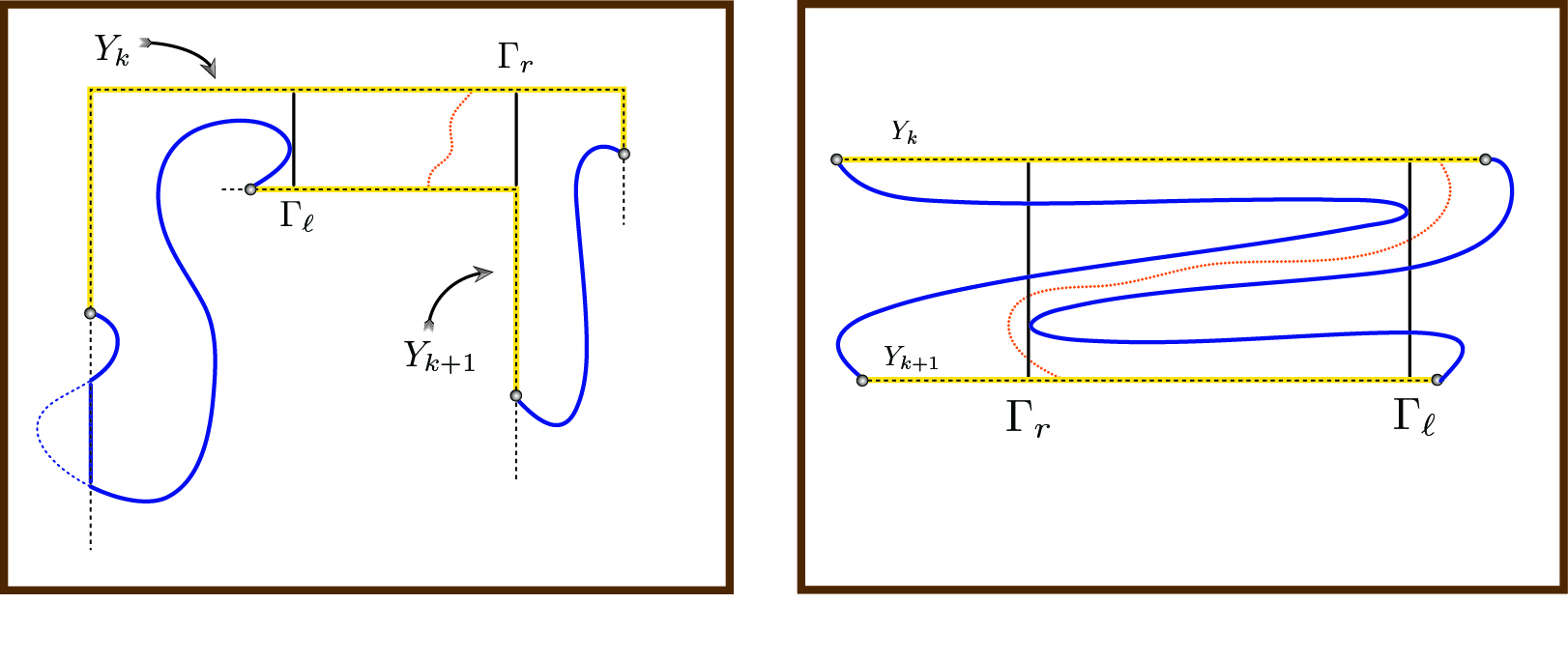
Figure 9: Setup described in the proof of Lemma 9 under simplified assumption that segments are fragments of squares. The constant $B$ here is envisioned to be about 2. Left: $\Gamma_{\ell}$ and $\Gamma_{r}$ situated as anticipated; $Y_{k}\leadsto Y_{k+1}$ is too likely. Right: $\Gamma_{\ell}$ and $\Gamma_{r}$ switched from anticipated placement; here $Y_{k}\leadsto Y_{k+1}$ is too unlikely.

We claim that the displacement (along $Y_{F}$) between $\Gamma_{\ell}$ and $\Gamma_{r}$ cannot exceed $B\cdot J_{F}$: first if $\Gamma_{\ell}$ were to the left of $\Gamma_{r}$, then the relevant yellow crossing probability in $A_{F}$ would be bounded from below by the easy way crossing of the topological rectangle bounded by $\Gamma_{\ell}$, $\Gamma_{r}$, $Y_{I}$ and $Y_{F}$. By the definition of $B$ this would exceed $1-\vartheta^{2}$, while by assumption, $A_{F}$ was constructed so that this yellow crossing probability could not exceed $1-\vartheta$. On the other hand, if $\Gamma_{\ell}$ were to the right of $\Gamma_{r}$, then any yellow crossing would now be forced to traverse the hard way along a topological rectangle with aspect ratio exceeding $B$, which again by definition of $B$ would be less than $\vartheta^{2}$ which is again contrary to the assumption concerning $A_{F}$.

Next, if possible, we will extend the portion of $Y_{F}$ which is in between $\Gamma_{\ell}$ and $\Gamma_{r}$ by an amount from $Y_{F}$ no more than an additional $B\cdot J_{F}$ on each side. Obviously, we do this only if space is available, otherwise, e.g., $\|Y_{F}\|_{\infty}$ is already less than $3B\cdot J_{F}$. We denote as necessary the bounding vertical segments at the end of the extensions by $\gamma_{\ell}$ and $\gamma_{r}$. In any case, these bounding segments $\gamma_{\ell},\gamma_{r}$, should they exist will hit $\mathscr{B}_{\ell}\cup\mathscr{B}_{r}$ and we will denote the portions of $\gamma_{\ell}$ and $\gamma_{r}$ which connect $Y_{F}$ to $\mathscr{B}_{\ell}$ and $\mathscr{B}_{r}$ by $\tau_{\ell}$ and $\tau_{r}$, respectively. The portion of $Y_{F}$ between $\tau_{\ell}$ and $\tau_{r}$ together with the $\tau$’s themselves constitute our effective region $Y_{F}^{(e)}$. (If no reconstruction is required, then we may consider $\tau_{\ell}=\tau_{r}=\emptyset$ and set $Y_{F}^{(e)}\equiv Y_{F}$.) Notice in particular that $\|\tau_{\ell}\|_{\infty}$ and $\|\tau_{r}\|_{\infty}$ cannot exceed $J_{F}$.

We now argue that the yellow crossings actually occur between the effective regions with high “conditional” probability. Consider the event $\mathscr{D}:=\{Y_{I}\leadsto Y_{F}\}\setminus\{Y_{I}\leadsto Y_{F}^{(e)}\}$. We first claim that the event $\mathscr{D}$ implies the existence of yellow and blue crossings in fragments of aspect ratio at least $B$ and therefore has probability less than $\vartheta^{4}$.

For simplicity, we will suppose that $\Gamma_{\ell}$ is the the left of $\Gamma_{r}$. In this case – assuming for non–triviality that $Y_{F}\neq Y_{F}^{(e)}$ – it may be further supposed without any additional loss of generality that $Y_{F}\setminus Y_{F}^{(e)}$ contains points to the right of $\Gamma_{r}$ from which the yellow crossing producing the event $\mathscr{D}$ emanates. Then, the fragment between $\gamma_{r}$ and $\Gamma_{r}$ has aspect ration $B^{\prime}$ with $B^{\prime}\geq B$. This fragment must be traversed the hard way by a yellow path in order that (this version of) the event $Y_{F}\setminus Y_{F}^{(e)}\leadsto Y_{I}$ occurs. But in addition, a similar sort of blue path must occur to separate the lowest version of said yellow path from the yellow boundary region between $\Gamma_{r}$ and $\gamma_{r}$; the intersection of these two path events has probability less than $\vartheta^{4}$ and so here the desired result has been established. Other cases are handled similarly.

The stated upper bound on the crossing probability follows more easily: it suffices to observe that the probability of a yellow connection between $Y_{I}$ and $\gamma_{\ell}$ or $\gamma_{r}$ by the choice of $B$ is bounded by $\vartheta^{2}$.

The General Case. The key point here is to have a tangible construction of $\Gamma_{r}$ and $\Gamma_{\ell}$ along with the associated $\tau_{r}$ and $\tau_{\ell}$, at which point the argument proceeds along the lines of the simplified case. We let $x_{r},\dots,\mathscr{B}_{r}$ be as defined before. Consider the composite curve consisting of $Y_{F},\mathscr{B}_{r}$, the portion of $\partial\Omega_{m}$ connecting $y_{r}$ to $y_{\ell}$ (not containing $\omega$) and $\mathscr{B}_{\ell}$. The curve described forms a closed loop whose interior we denote by $\mathscr{C}$ and note particularly that $Y_{I}$ must lie in $\mathscr{C}$.

We emphasize that by definition of the sliding procedure, the $d_{\infty}^{A_{F}}$– distance of every element of $Y_{F}$ to some element of $Y_{I}$ is within a few lattice spacings of $J_{F}$ (small discrepancies may arise due to the extended SIU’s and certain lattice details). Thus let $J_{F}^{\prime}=J_{F}+c$ – for some constant $c$ of order unity – denote the maximal such distance. Let $x_{\alpha}$ and $x_{\beta}$ denote two points along $Y_{F}$ with $x_{\alpha}$ to the right of $x_{\beta}$ and such that $d_{\infty}^{A_{F}}(x_{\alpha},x_{\beta})>2\cdot J_{F}^{\prime}$; thus the boxes of side $2J_{F}^{\prime}$ (i.e., “radius” $J_{F}^{\prime}$) centered about these points are disjoint. Note that $Y_{I}$ must visit both of these boxes; for simplicity, let us, if necessary, shrink these boxes by a few lattice spacings (no more than $c$) so that $Y_{I}$ can only visit the surface of these boxes. We denote the boxes centered at $x_{\alpha}$ and $x_{\beta}$ by $\mathfrak{b}_{\alpha}$ and $\mathfrak{b}_{\beta}$, respectively.

Our claim is that (regarding $Y_{I}$ as moving from $y_{r}$ to $y_{\ell}$) $Y_{I}$ must visit $\mathfrak{b}_{\alpha}$ before it visits $\mathfrak{b}_{\beta}$. Indeed, supposing to the contrary that $Y_{I}$ visits $\mathfrak{b}_{\beta}$ first, then it is noted that the curve consisting of the portion of $Y_{I}$ from $y_{r}$ till it hits $\mathfrak{b}_{\beta}$ and portions of $\partial\mathfrak{b}_{\beta}$ (plugging into $Y_{F}$) would divide $\mathscr{C}$ into two disjoint components, one containing $x_{\alpha}$ (on its boundary) and the other containing $y_{\ell}$ (on its boundary). Moreover, the former component contains all of $\mathfrak{b}_{\alpha}\cap\mathscr{C}$. Thus $Y_{I}$ could not possibly then proceed to visit $\partial\mathfrak{b}_{\alpha}$ without crossing the aforementioned separating curve and/or $\partial\mathscr{C}$.

Now consider a sequence of successive non–overlapping boxes $\mathfrak{b}_{1},\mathfrak{b}_{2},\dots\mathfrak{b}_{q}$ centered on points in $Y_{F}$ oriented from right to left, so that $\mathfrak{b}_{1}$ is centered at $x_{r}$. All these boxes have diameter approximately $2J_{F}^{\prime}$ which have been tuned, as above, so that $Y_{I}$ just visits their surfaces. Let us look at the last such box which intersects $\mathscr{B}_{r}$ and denote it by $\mathfrak{b}_{s}$. Due to the above claim, it is clear that $\mathfrak{b}_{1},\dots,\mathfrak{b}_{s-1}$ are all intersected by $\mathscr{B}_{r}$ and, moreover, within each box, the relevant portion of $\mathscr{B}_{r}$ separates $Y_{F}$ from $Y_{I}$ (at least twice). Indeed, first consider paths $\widetilde{\mathscr{B}}_{r}$ and $\widetilde{\mathscr{B}}_{\ell}$ outside of $\Omega_{m}$ which do not intersect the $\mathfrak{b}$ boxes and also connect $x_{r}$ to $y_{r}$ and $x_{\ell}$ to $y_{\ell}$, respectively. Next consider the domain bounded by $Y_{I}\cup Y_{F}\cup\widetilde{\mathscr{B}}_{r}\cup\widetilde{\mathscr{B}}_{\ell}$; the curve $\mathscr{B}_{r}$ (and later also $\mathscr{B}_{\ell}$) must lie within this domain. Now on each $\mathfrak{b}_{j}$, there are two portions of $\partial\mathfrak{b}_{j}$ connecting $Y_{I}$ to $Y_{F}$ and both of these separate $y_{r}$ from $\mathfrak{b}_{s}$ within the domain just described.

We will now define $\Gamma_{r}$ to be the portion of $\partial\mathfrak{b}_{s+1}$ which is inside $A_{F}$ and connects $Y_{F}$ to $Y_{I}$. (There are, in fact at least two two choices; to be definitive, we choose, starting from $Y_{F}$, the“rightmost”.) As before, we move from $\mathfrak{b}_{s}$ to $\mathfrak{b}_{s-k}$ where $\mathfrak{b}_{s-k}$ is the nearest box whose $d_{\infty}^{A_{F}}$– distance from $\mathfrak{b}_{s}$ is greater than $B\cdot J_{F}$. The topological statements above about $\mathscr{B}_{r}$ then permits us to define $\tau_{r}$ as any (lattice) path between the center of $\mathfrak{b}_{s-k}$ and $\mathscr{B}_{r}$ within the box. Note in the above that we have tacitly assumed $s\geq 1$, otherwise, e.g., $\tau_{r}=\emptyset$. Finally, $\Gamma_{\ell}$, etc., are defined analogously. With these tangible definitions of $\Gamma_{r}$, $\Gamma_{\ell}$, $\tau_{r}$ and $\tau_{\ell}$, the proof concludes mutatis mutantis along the lines of the simplified case. Notice that again, $\|\tau_{\ell}\|_{\infty},\|\tau_{r}\|_{\infty}\leq J_{F}+c\approx J_{F}$ and so the diameter of $Y_{F}^{(e)}$ is bounded above as in the statement of this lemma.

As for the stated lower bound on the diameter, let us first note, supposing $Y_{F}^{(e)}=Y_{F}$, that since $\|Y_{F}\|_{\infty}\geq d_{\infty}^{A_{F}}(\mathscr{B}_{\ell},\mathscr{B}_{r})$, if it were the case that $\|Y_{F}\|_{\infty}<B^{-1}\cdot J_{F}$, then by the choice of $B$ we would conclude that the blue crossing probability is in excess of $1-\vartheta^{2}$, which is impossible. Therefore, $\|Y_{F}\|_{\infty}\geq B^{-1}\cdot J_{F}$. On the other hand, if we actually had to perform the effective regions construction, then we clearly have $\|Y_{F}^{(e)}\|_{\infty}\geq B\cdot J_{F}$. ∎

We will now address the cases where a successful construction of a $Y_{F}$ requires a backsliding construction, as featured in Lemma 5.2 and the discussions thereafter. The relevant barrier segment $Z_{F}$ will be constructed by a modification of $Y_{F,L}$, where $L$ is the smallest integer larger than $J_{F}/2$.

We observe that by construction, each box of size $L$ around an element of $Y_{F,L}$ is visited by $Y_{I}$, so with the meaning of $\mathfrak{b}_{j}$ the same as in the above proof, we let $\mathfrak{b}_{\alpha}$ be the leftmost box which is not intersected by $\mathscr{B}_{r}$ and $\mathfrak{b}_{\beta}$ the rightmost box which is not intersected by $\mathscr{B}_{\ell}$. If it is the case that $\alpha<\beta$ (considering the orientation to be from right to left) then we perform effective region construction on $Y_{F,L}$ (here we clearly have $\partial\Omega_{m}$ sufficiently close to $Y_{F,L}$ so that the construction can be performed with $\|\tau_{\ell}\|_{\infty}$ and $\|\tau_{r}\|_{\infty}$ remaining well–controlled) and set $Z_{F}$ to be the resulting modified segment.

We are left with the case that $\alpha>\beta$; here we will set $Z_{F}\equiv Y_{F,L}$. But let us note the following fact (which is only non–trivial if $\beta-\alpha>B$): if $w_{F,L}\subseteq Y_{F,L}$ is any connected subsegment which traverses more than $B$ of the $\mathfrak{b}_{j}$ boxes between $\mathfrak{b}_{\alpha}$ and $\mathfrak{b}_{\beta}$, then

$$\mathbb{P}(Y_{I}\leadsto w_{F,L})>1-\vartheta^{2},$$

where the above crossing is allowed to take place anywhere in the region bounded by $Y_{I},Y_{F,L}$ and the relevant portions of $\partial\Omega_{m}$. Indeed this follows since to prevent such a connection entails a long way blue crossing with aspect ration in excess of $B$.

Proposition 5.5

In the cases where $Y_{F}$ must be obtained from $Y_{I}$ via a backsliding procedure as described following Lemma 5.2 and above, there exists an $m$ such that $G_{m}^{(F)}$ has the following properties:

1) $\mathbb{P}(Y_{I}\leadsto G_{m}^{(F)})\in(\vartheta,1-\vartheta)$;

2) there is some constant $\kappa>0$ such that $\|G_{m}^{(F)}\|_{\infty}\leq\kappa B\cdot L$.

Proof.

Let us temporarily denote by $\widetilde{Y}_{F}$ the first successor segment such that $\mathbb{P}(Y_{I}\leadsto\widetilde{Y}_{F})<\vartheta$ (i.e., the suppressed second index is approximately equal to $2L$). First, if necessary, we perform effective region like construction on $\widetilde{Y}_{F}$: again, we reiterate that if the relevant $\Gamma_{\ell}$ lies to the right of $\Gamma_{r}$, then the relevant $\tau_{\ell}$ and $\tau_{r}$ are well controlled and the diameter of the effective region obeys the bounds stated in Lemma 5.4 (relative to $\widetilde{J}_{F}$ which is the relevant separation distance between $Y_{I}$ and $\widetilde{Y}_{F}$). On the other hand, if $\Gamma_{\ell}$ is to the left of $\Gamma_{r}$, then the observation immediately preceding the statement of this proposition implies that the separation between $\Gamma_{\ell}$ and $\Gamma_{r}$ cannot exceed $B\cdot L$ and, if necessary, we may perform an additional effective region construction.

In any case, as in Lemma 5.4, we have manufactured a $\widetilde{Y}_{F}^{(e)}$ whose diameter does not exceed $\kappa^{\prime}B\cdot L$. Now we will carry out the backsliding procedure starting with $\widetilde{Y}_{F}^{(e)}$ with the barrier $Z_{F}$ as described above. We observe that after approximately $L$ iterations, we will have reached $Z_{F}$. We will not do more than an additional $\kappa^{\prime}B\cdot L$ iterations (in order to achieve the crossing probability criterion) because if so, we would have subsumed a portion of $Z_{F}$ at least this large (or perhaps all of it) and, by the observation immediately preceding the proposition, the crossing probability from $Y_{I}$ would exceed $1-\vartheta^{2}$. Thus, $m$ is certainly less than $(\kappa^{\prime}B+1)\cdot L$. It follows that $\|G_{m}^{(F)}\|_{\infty}$ is less than $\|\widetilde{Y}_{F}^{(e)}\|_{\infty}+c\cdot m$, where the constant $c$ corresponds to increase in diameter due to the $d_{\infty}$–neighborhood construction. We thus have that $\|G_{m}^{(F)}\|_{\infty}$ is less than or equal to $\kappa B\cdot L$ for some constant $\kappa$, as stated. ∎

We can now set $Y_{F}$ to be equal to the $G_{m}^{(F)}$ existentiated above and set $J_{F}$ to be equal to $L$. For future reference we will adopt $\kappa$ as the constant bounding the diameter of all such regions.

5.3.3 The $R$–Construction (percolative boxes)

Our objectives will eventually be achieved by establishing the existence of monochrome percolation connections between e.g., (the vicinity of) $\omega$ and the central region $\mathcal{D}_{\Delta}$. This will be accomplished by establishing a grid of contiguous boxes within each of the successor ring fragments. This entails a suitable modification of $Y_{F}^{(\cdot)}$, which will then define the final ring fragment of interest. Most pertinently, as will emerge later, the sizes of the boxes in neighboring fragments will differ by at most a uniform scale factor.

Remark 5.6.

We remark that in the forthcoming use of boxes, as far as connectivity properties are concerned, all notions are inherited from the standard 2D square site lattice, e.g., boxes are connected if they share an edge in common and, dually, $*$–connected means an edge or corner in common.

Suppose now that $Y_{I},Y_{F}$ and $J_{F}$ are such that the conclusion of Lemma 5.4 holds (particularly, $\mathbb{P}(Y_{I}\leadsto Y_{F})\in(\theta^{\prime\prime},1-\theta^{\prime\prime})$). Let us tile the region enclosed by $Y_{I}$ and $Y_{F}$ (i.e., $A_{F}$) by boxes of size $2^{-r}\cdot J_{F}$ for some $r>0$. The boxes under consideration will include all boxes whose closure intersects the closure of $A_{F}$; the precise value of $r$ will be specified later. We remark that these boxes will be a super–grid for boxes of the ultimate small scale which will be $2^{-2r}\cdot J_{F}$. We start with the larger scale:

Claim. There exists some fixed $r_{0}\equiv r(\theta^{\prime\prime})>0$ such that if $r>r_{0}$ then among the aforementioned boxes of scale $2^{-r}\cdot J_{F}$ there is a connected path between $Y_{I}$ and $Y_{F}$ by boxes which do not intersect the blue boundaries.

Proof of Claim. Let $\beta$ denote any box which intersects $\mathscr{B}_{\ell}$. Then we assert, for $r$ chosen suitably large, that $\beta$ or any box in its $*$–connected neighborhood does not meet $\mathscr{B}_{r}$. Indeed, supposing to the contrary, let us consider the $r-2$ annuli of doubling sizes $2^{-r}\cdot J_{F}\times[4,\dots,2^{r-1}]$ with $\beta$ at the center. Since we have started at $4\times 2^{-r}\cdot J_{F}$ the inner ring always contains the $*$–neighborhood of $\beta$ and since we have ended at $\frac{1}{2}\cdot J_{F}$, it cannot be the case that both $Y_{F}$ and $Y_{I}$ penetrate (any of) these annuli. In each such annulus, by weak scale invariance of critical percolation, a blue circuit independently exists with probability at least some $\lambda$ and each such blue circuit would connect $\mathscr{B}_{\ell}$ to $\mathscr{B}_{r}$ in $A_{F}$, thereby preventing a yellow crossing. But then for $r$ large enough, the yellow crossing probability would be too small; indeed,

$$\theta^{\prime\prime}\leq\mathbb{P}(Y_{I}\leadsto Y_{F})\leq(1-\lambda)^{r-2}.$$

The above defines $r_{0}$: $(1-\lambda)^{r_{0}-2}:=\theta^{\prime\prime}$ and so the assertion has been established. Now the claim will (eventually) follow: let $y_{r}$ and $y_{\ell}$ denote the left and right endpoints of $Y_{I}$ and moving from $y_{\ell}$ to $y_{r}$ along $Y_{I}$ let $\beta_{\ell}$ denote the last (rightmost) box intersected by $Y_{I}$ which also intersects $\mathscr{B}_{\ell}$. We similarly define $\beta^{\prime}_{\ell}$ along $Y_{F}$ and $\beta_{r},\beta_{r}^{\prime}$ relative to $\mathscr{B}_{R}$. We further define $\mathbf{Y}_{I}$, $\mathbf{Y}_{F}$, $\mathbf{B}_{\ell}$ and $\mathbf{B}_{r}$: the set $\mathbf{Y}_{I}$ consists of those boxes which meet the portion of $Y_{I}$ which is after its last exit from $\beta_{\ell}$ and before its first entrance into $\beta_{r}$. Similarly, let $\mathbf{B}_{\ell}$ denote those boxes which meet the portion of $\mathscr{B}_{\ell}$ after its last exit from $\beta_{\ell}$ and before its first entrance into $\beta_{\ell}^{\prime}$. Similarly for $\mathbf{Y}_{F}$ and $\mathbf{B}_{r}$.

It is seen that save for the four corners mentioned, all these sets are disjoint: the $\mathbf{Y}$ pair are “well separated”, the $\mathbf{B}$ pair are (not quite as well) separated due to the above assertion and, e.g., $\mathbf{Y}_{I}$ and $\mathbf{B}_{\ell}$ are disjoint save for $\beta_{\ell}$ essentially by definition. Now these sets, which are $*$–connected objects (although not necessarily $*$–connected paths) certainly form the boundary of a “crossing problem arena” – we temporarily delete from consideration all other boxes which meet $\partial A_{F}$. The desired crossing exists because, due to the first assertion, we have, for example, that the $*$–connected boundary of $\mathbf{B}_{\ell}$ is disjoint from $\mathbf{B}_{r}$. ∎

Remark 5.7.

For the benefit of the forthcoming, the above display should be modified to read $(1-\lambda)^{r}<\vartheta^{2}\ll\theta^{\prime\prime}$ – where in addition, we have now stipulated $\vartheta\sim\theta^{\prime\prime}\ll 1$. This will set our scales. Thus we envision $2^{r}$ as comparable to $B$ but, in any case, we certainly have

$$2^{r}\geq B$$

We will now define the current modification to $Y_{F}$:

Definition of $Y_{F}^{(b)}$. Consider now the grid of scale $2^{-2r}\cdot J_{F}$ – considerably smaller than the previous grid. Here it is stipulated that $r$ (with $r>r_{0}$) has been chosen so as to satisfy

$$(1-\lambda)^{r-1}<(\theta^{\prime\prime})^{2},$$

with $\lambda$ being the probability of a monochrome circuit in an annulus where the outer scale is twice the inner scale. Again we consider the (closed) boxes which have non–zero intersection with the region $A_{F}$ – and for the immediate future, no others. From this set we delete all boxes which have non–empty intersection with $Y_{F}$ and their $*$–neighboring boxes.

The remaining boxes may now consist of several components. Nevertheless, we may temporarily consider all boxes with at least one edge not shared by another box in the collection to be a boundary box. These “exposed” box–edges form closed circuits – the edge boundaries of the components. Among these circuits there is to be found a unique path which begins on $\mathscr{B}_{\ell}$, ends on $\mathscr{B}_{r}$, have no other encounters with either of the $\mathscr{B}$’s and which is disjoint from the old $\mathbf{Y}_{I}$. This special path is characterized as follows; we consider a larger set of paths which are allowed to use edges of any box. These paths have the same general description used above: they connect $\mathscr{B}_{\ell}$ to $\mathscr{B}_{r}$ and consist of whole (box) edges save, possibly, for the first and last wherein occurs the only encounter with $\mathscr{B}_{\ell}\cup\mathscr{B}_{r}$. Such a set is obviously non–empty since $\mathscr{B}_{\ell}$ is connected to $\mathscr{B}_{r}$ by boxes (even of the larger scale) and the paths are partially ordered with respect to their separation from $Y_{I}$. The special path is the one that is “furthest” from $Y_{I}$.

One final modification is required. Consider the boxes which share at least one edge (or fragment thereof) with the aforementioned path. By the ordering considerations of the construction, each edge belongs to a unique box (the collection of which in fact form a $*$–connected chain). Moving from left to right along the path, we define, as in the context of the larger grid, the box $\mathfrak{b}_{\ell}$ to be the rightmost of the boxes which intersect $\mathscr{B}_{\ell}$ and similarly for $\mathfrak{b}_{r}$. We now consider the portion of the path connecting $\mathfrak{b}_{\ell}$ to $\mathfrak{b}_{r}$ and adjoin to it the box edges (partial or otherwise) of $\mathfrak{b}_{\ell}$ and $\mathfrak{b}_{r}$ so that overall we have reconstituted a connection between $\mathscr{B}_{\ell}$ and $\mathscr{B}_{r}$. This final step should be enacted by choosing the path along the box edges to be “as far away” from $Y_{I}$ as possible.

The definition is essentially complete, the above constructed path constitutes the segment $Y_{F}^{(b)}$. The region $A_{F}^{(b)}$ is the topological rectangle with boundaries $Y_{I}$, $Y_{F}^{(b)}$ and the appropriate portions of $\mathscr{B}_{\ell}$ and $\mathscr{B}_{r}$ which connect these segments. Finally, we use the notation

$$b_{F}:=2^{-2r}\cdot J_{F}$$

for the scale – sidelength – of the individual boxes.

Remark 5.8.

Let us note for future reference that by virtue of having used $*$–connected neighborhoods, it is the case that there is a full layer of connected boxes separating $Y_{F}$ from $Y_{F}^{(b)}$. The fact that there is a full layer is clear; the fact that this layer is connected follows from the observation that the boxes which intersect $Y_{F}$ were, certainly, $*$–connected, so the layer represents a portion of the dual circuit surrounding this set.

We now observe that $Y_{F}^{(b)}$, $A_{F}^{(b)}$ etc., have various anticipated properties:

Proposition 5.9

Consider the boundary boxes of $A_{F}^{(b)}$ that share portions of their boundary with $Y_{F}^{(b)}$. Then these boxes form a $*$–connected cluster – and hence $Y_{F}^{(b)}$ itself is connected. Moreover, each such box is connected by a (connected) path of full boxes to boxes which intersect $Y_{I}$ with a path length – measured in number of boxes – which does not exceed some universal constant $\textsc{l}\in(0,\infty)$.

Proof.

It is noted that by construction, $Y_{F}^{(b)}$ is constituted from a non–repeating sequence of attached box edges all of which are complete save the first and last. Therefore, it is manifestly connected and, moreover, the boxes which contribute boundary elements to this segment form a $*$–connected chain running from $\mathfrak{b}_{\ell}$ to $\mathfrak{b}_{r}$, inclusive. We denote this chain by $\mathbf{y}_{F}$ and define $\mathbf{y}_{I}$, $\mathbf{b}_{\ell}$ and $\mathbf{b}_{r}$ in the same fashion as their upper case counterparts were defined using the larger scale boxes. The region bounded by $\mathbf{y}_{F}$ and appropriate elements of the other sets $\mathbf{y}_{I}$, $\mathbf{b}_{\ell}$ and $\mathbf{b}_{r}$ form a topological rectangle along with associated boundaries so that opposing pairs are well separated (as in the claim for the larger scale boxes) and hence any box in $\mathbf{y}_{F}$ can be connected to some box in $\mathbf{y}_{I}$.

Finally, concerning the length of the connection, let us provide a crude estimate: it is known that the diameter of $Y_{F}^{(b)}$ is bounded by $\|Y_{F}\|_{\infty}\leq\kappa B\cdot J_{F}$ (by Lemma 5.4 and Proposition 5.5); moreover, every point on $Y_{F}^{(b)}$ is separated from some point on $Y_{I}$ by $d_{\infty}$–distance some constant times $\kappa B\cdot J_{F}$. Thus, a box which is a reasonable multiple of $B\cdot J_{F}$ centered about $Y_{F}$ – let us call it $\mathbb{B}$ – contains all of $Y_{F}$ and paths between every point on $Y_{F}$ and some point on $Y_{I}$ and a substantial neighborhood (e.g., larger than $J_{F}$) of these paths.

Now consider any “microscopic” path $\mathscr{P}$ in $A_{F}$ between a point on $Y_{F}$ and some point on $Y_{I}$ contained in $\mathbb{B}$ and let us denote by $\mathfrak{b}_{\mathscr{P}}$ the set of small boxes visited by $\mathscr{P}$. Of course, $\mathfrak{b}_{\mathscr{P}}$ may contain boundary boxes from $\mathbf{b}_{\ell}$ and/or $\mathbf{b}_{r}$; however, since these are well–separated, the $*$–connected closure of $\mathfrak{b}_{\mathscr{P}}$ manifestly contains a connected path of full boxes between $\mathbf{y}_{F}$ and $\mathbf{y}_{I}$ (indeed, the $*$–connected closure of e.g., $\mathbf{b}_{\ell}$ itself consist of full boxes). Finally, it is certainly the case that any such path cannot possibly consist of more boxes than the total number of boxes in the aforementioned bounding set $\mathbb{B}$. Since both $\mathbb{B}$ and the small boxes have area proportional to a universal constant times $J_{F}^{2}$, the result follows for some l. ∎

Our next claim is that the replacement of $Y_{F}$ by $Y_{F}^{(b)}$ does not substantially alter the yellow crossing probability:

Claim. Suppose $\mathbb{P}(Y_{I}\leadsto Y_{F})\in(\theta^{\prime\prime},1-\theta^{\prime\prime})$, then

$$\theta^{\prime\prime}\leq\mathbb{P}(Y_{I}\leadsto Y_{F}^{(b)})<\frac{1-\theta^{\prime\prime}}{(1-(\theta^{\prime\prime})^{2})^{2}}\approx 1-\theta^{\prime\prime}+2(\theta^{\prime\prime})^{2}.$$

Proof of Claim. The lower bound is immediate since a crossing from $Y_{I}$ to $Y_{F}$ certainly implies a crossing to $Y_{F}^{(b)}$. The upper bound follows from an easy continuation of crossings argument: indeed, consider e.g., the “left” endpoint of $Y_{F}$ whose grid box we surround by an annulus with inner scale $2^{r}\cdot b_{F}$ and outer scale $2^{r}$ times this inner scale. Let us consider the event $\mathbb{G}$ that the rightmost crossing from $Y_{I}$ to $Y_{F}^{(b)}$ is outside the inner square defining the above annulus. Then, we have at least $r$ independent chances – by setting up independent annuli – to continue the rightmost crossing to $Y_{F}$. This continuation therefore happens with (conditional) probability in excess of $1-(\theta^{\prime\prime})^{2}$ by the choice of $r$ and so

$$\mathbb{P}(\{Y_{I}\leadsto Y_{F}\mid\{Y_{I}\leadsto Y_{F}^{(b)}\}\cap\mathbb{G})>1-(\theta^{\prime\prime})^{2}.$$

On the other hand, let $\mathbb{O}_{Q}$ denote the event of a yellow circuit somewhere inside the $b_{F}\cdot 2^{r}\times b_{F}\cdot 2^{2r}$ annulus. We note that should the event $\mathbb{O}_{Q}$ occur, then, indeed, the rightmost crossing is to the right of this inner square and so by the choice of $r$, $\mathbb{P}(\mathbb{G})\geq\mathbb{P}(\mathbb{O}_{Q})>1-(\theta^{\prime\prime})^{2}$

The desired inequality now follows:

$$\begin{split}\mathbb{P}(Y_{I}\leadsto Y_{F})&\geq\mathbb{P}(Y_{I}\leadsto Y_{F}\mid\{Y_{I}\leadsto Y_{F}^{(b)}\}\cap\mathbb{G})\cdot\mathbb{P}(\{Y_{I}\leadsto Y_{F}^{(b)}\}\cap\mathbb{G})\\ &>(1-(\theta^{\prime\prime})^{2})^{2}\cdot\mathbb{P}(Y_{I}\leadsto Y_{F}^{(b)}).\end{split}$$

Here to arrive at the last line we have used the FKG inequality. ∎

Corollary 5.10

Consider the curve, denoted by $\overline{Y}_{F}^{(b)}$ which consists of the outer edges (i.e., closer to $Y_{F}$) of the boxes which share an (inner) edge with a box in $\mathbf{y}_{F}$ and attached to $\mathscr{B}_{\ell}$ and $\mathscr{B}_{r}$ by an analogous procedure as was used for $Y_{F}^{(b)}$. Then

$$\mathbb{P}(\overline{Y}_{F}^{(b)}\leadsto Y_{F}^{(b)})>1-(\theta^{\prime\prime})^{2}.$$

Proof.

This follows directly from the above argument using the observation that $\overline{Y}_{F}^{(b)}$ separates $Y_{F}$ from $Y_{F}^{(b)}$. ∎

Remark 5.11.

We remark that we should think of the above claim “dually”, i.e., that the complementary bound

$$\theta^{\prime\prime}-c_{2}(\theta^{\prime\prime})^{2}<\mathbb{P}(\mathscr{B}_{\ell}^{\prime}\leadsto\mathscr{B}_{r}^{\prime})\leq 1-\theta^{\prime\prime}$$

(for $\theta^{\prime\prime}$ small and some constant $c_{2}$) holds for blue crossings; here $\mathscr{B}_{\ell},\mathscr{B}_{r}$ now denote the appropriate “left” and “right” blue boundaries of the topological rectangle formed by $Y_{I}$ and $Y_{F}^{(b)}$. Indeed, as will unfold below, all that is actually used for yellow crossings is the ability to cross these regions via paths inside the boxes with a probability which is independent of the details of the region.

5.4 Induction

We are now ready to assemble all ingredients and describe the full inductive procedure. Our goal is to show that there are box connections between all successive yellow segments and that the box scale of neighboring layers do not differ by too much.

First let us set out the base case for our induction. Let $Y_{0}:=\partial S_{0}(\omega)\cap\partial\mathcal{D}_{\Delta}$ be as described before. If $\mathbb{P}(Y_{0}\leadsto\omega)\geq\vartheta$, then stop. (Indeed, this is one of the stopping criterion for our iteration and if it actually occurs on the first step, then clearly the lattice spacing is too large to be worthy of any detailed consideration.) Otherwise, let us perform the $S,Q,R$–constructions to yield some $\widehat{Y}_{1}$ so that $\mathbb{P}(\widehat{Y}_{1}\leadsto Y_{0})\in(\theta^{\prime\prime},1-\theta^{\prime\prime})$. Recall that here $\theta^{\prime\prime}$ may differ from $\vartheta$ due to the $O(\vartheta^{2})$ errors in the $Q,R$–construction sections. It is noted that since $\mathcal{D}_{\Delta}$ has a radius half the maximal amount, for judicious choice of $\vartheta$, the ancillary constructions, in particular the $Q$–construction, are actually not necessary.

We will assume the existence of segments

$$P_{0}\equiv\widehat{Y}_{0},~{}P_{1}\equiv\widehat{Y}_{1},~{}\dots,~{}P_{k-1}\equiv\widehat{Y}_{k-1},~{}T_{k}\equiv\widehat{Y}_{k}.$$

(Here the $\widehat{~}{}$ denotes modifications to the original segments $Y_{\ell}$ from the $Q,R$–constructions.) The following are our inductive hypotheses:

0) $T_{k}$ is the box construction version of some $Y_{k}$ and there is some $\overline{Y}_{k}$ which is the $d_{\infty}$– neighborhood boundary of $T_{k}$ such that

i) $\mathbb{P}(\overline{Y}_{k}\leadsto T_{k})\geq 1-(\theta^{\prime\prime})^{2}$ (by Corollary 5.10);

ii) $d_{\infty}(T_{k},Y_{k})>b_{k}$ (by Remark 5.8);

1) the following conclusions hold for $P_{k-1}$ and $T_{k}$:

i) $\mathbb{P}(P_{k-1}\leadsto T_{k})\in(\theta^{\prime\prime},1-\theta^{\prime\prime})$;

ii) all of $T_{k}$ can be connected to $P_{k-1}$ via boxes of size $b_{k}$ completely unobstructed by $\partial\Omega_{m}$ and further the number of boxes required for such a connection is not in excess of l (by Proposition 5.9);

iii) it is the case that (see the effective regions construction subsubsection)

$$B^{-1}\cdot J_{k}\leq\|P_{k-1}\|_{\infty}\leq 2^{2r+1}(\kappa B)\cdot J_{k},~{}~{}~{}B^{-1}\cdot J_{k}\leq\|T_{k}\|_{\infty}\leq\kappa B\cdot J_{k}.$$

2) the conclusions of 1.ii) and 1.iii) also hold for (prior) successive segments $P_{\ell-1},P_{\ell}$, $1\leq\ell\leq k-1$; also a weakened version of 1.i) holds for these prior segments: $\mathbb{P}(P_{j-1}\leadsto P_{j})\leq 1-\theta^{\prime\prime}$ (which we think of as a lower bound on the blue crossings).

Here the letter $P$ denotes what is considered a permanent yellow segment whereas $T$ denotes a temporary segment. Let us note that we will not require the lower bound on yellow crossing probabilities per se except for the last layer consisting of $P_{k-1},T_{k}$.

Step 1. We first construct some segment $Y_{k+1}$ by sliding $T_{k}$ towards $\omega$ and backsliding if necessary so that

$$\mathbb{P}(T_{k}\leadsto Y_{k+1})\in(\vartheta,1-\vartheta).$$

Step 2. Next we perform the effective regions construction and the box construction to yield $\widehat{Y}_{k+1}$ so that $\mathbb{P}(T_{k}\leadsto\widehat{Y}_{k+1})\in(\theta^{\prime\prime},1-\theta^{\prime\prime})$, $\|\widehat{Y}_{k+1}\|_{\infty}\leq\kappa B\cdot J_{k+1}$ and there are suitable box connections between $T_{k}$ and $\widehat{Y}_{k+1}$ with boxes of scale $b_{k+1}=2^{-2r}\cdot J_{k+1}$ (see Lemma 5.4, Proposition 5.5 and Proposition 5.9). Notice that we also immediately have from the bound on the crossing probabilities and Lemma 5.4 that

$$\|T_{k}\|_{\infty}\geq B^{-1}\cdot J_{k+1},~{}~{}~{}\|Y_{k+1}\|_{\infty}\geq B^{-1}\cdot J_{k+1}.$$

Step 3. We have now satisfied items 1.i) and 1.ii) of the inductive hypothesis for the layer $(T_{k},\widehat{Y}_{k+1})$.

Step 4. Now we will verify item 1.iii). First we claim that $J_{k+1}>b_{k}/2$.

Indeed, recall that there is a connected neighborhood of boxes separating $T_{k}$ from $Y_{k}$ (again see Remark 5.8). The (outer) boundary of this neighborhood is $\overline{Y}_{k}$ which by item 0.i) is connected to $T_{k}$ with too high a probability to consider stopping the process until at least some portion of the evolving neighborhood boundary reaches past it. However, by the nature of the neighborhood sliding construction the entire evolving boundary pushes through this curve coherently. So if the construction of $Y_{k+1}$ does not entail a backsliding, then the result immediately follows, in fact without the factor of two. Now if a backsliding were required, then recall that we used $Y_{k+1,L_{k+1}}$ as a barrier (here $L_{k+1}$ is the closest integer to $J_{k+1}/2$, as described in the discussions preceding Proposition 5.5) and so the claim follows by item 0.ii).

Item 1.iii) has now been verified since we now have $\|T_{k}\|_{\infty}\leq\kappa B\cdot J_{k}\leq 2^{2r+1}(\kappa B)\cdot J_{k+1}$. All induction hypotheses have been verified, so we set $P_{k}\equiv T_{k}$ and $T_{k+1}\equiv\widehat{Y}_{k+1}$.

The induction can now be continued towards $\omega$, starting with $P_{k}$ and $T_{k+1}$, provided that $\mathbb{P}(T_{k+1}\leadsto\omega)<\vartheta$ and $k+1\leq\Gamma\cdot\log n$, with $\Gamma$ as in the statement of Theorem 3.10 – otherwise we stop.

Remark 5.12.

We note particularly that from item 3 in step 4 of the induction, the percolating boxes are connected going from one layer to the next.

Also, for notational convenience, in the statement of Theorem 3.10, we have reverted back to using $\vartheta$ (so $\vartheta$ there corresponds to $\theta^{\prime\prime}$ here).

5.5 A Refinement

We will require one additional property of these Harris systems. First let us define some terminology:

Definition 5.13.

Let $\Omega\subset\mathbb{C}$ be a bounded, simply connected domain and $\Omega_{m}$ some interior discretization of $\Omega$. For $\omega\in\Omega_{m}$, consider the inductive construction as described, yielding $P_{1},P_{2},$ etc., until the crossing probability between $\omega$ and the last $P_{\ell}$ is less than $\vartheta$ – indicating that we have approximately reached the unit scale – or until we have succeeded a sufficient number of segments.

We remind the reader that we refer to the topological rectangles formed by successive $P_{\ell}$’s as Harris rings and the amalgamated system of these segments around $\omega$ the Harris system stationed at $\omega$.

For our purposes we will also need to show that for $n$ sufficiently large, for the marked point corresponding to $A$, the relevant Harris segments have endpoints lying in the anticipated boundary regions:

Lemma 5.14

Let $\Omega\subseteq\mathbb{C}$ be a bounded simply connected domain with marked boundary prime ends $A,B,C,D\in\partial\Omega$ (in counterclockwise order) and suppose $\Omega_{m}$ is an interior approximation to $\Omega$ with $A_{m},B_{m},C_{m},D_{m}\in\partial\Omega_{m}$ approximating $A,B,C,D$. Consider the hexagonal tiling problem studied in [14] or the flower models introduced in [10] (in which case we assume the Minkowski dimension of $\partial\Omega$ is less than 2) and the Harris system stationed at $A_{m}$. Then there is a number $v_{A}$ such that for all $m$ sufficiently large, all but $v_{A}$ of the Harris segments form conduits from $[D_{m},A_{m}]$ to $[A_{m},B_{m}]$. More precisely, under uniformization, there exists some $\eta>0$ such that all but $v_{A}=v_{A}(\eta)$ of these segments begin and end in the $\eta$–neighborhood of the pre–image of $A$.

Proof.

Let $\varphi:\mathbb{D}\rightarrow\Omega$ be the uniformization map with $\varphi(0)=z_{0}$ for some $z_{0}\in\mathcal{D}_{\Delta}$ and let $\zeta_{A},\zeta_{B},\zeta_{C},\zeta_{D}$ denote the pre–images of $A,B,C,D$, respectively. Let $\eta>0$ denote any number smaller than e.g., half the distance separating any of these pre–images. Let $N_{\eta}(\zeta_{A})$ denote the $\eta$–neighborhood of $A$ and let $\{r_{d},r_{b}\}$ denote the pair $N_{\eta}(\zeta_{A})\cap\partial\mathbb{D}$ with $r_{d}$ in between $\zeta_{A}$ and $\zeta_{D}$ and $r_{b}$ between $\zeta_{A}$ and $\zeta_{B}$. Similarly, about the point $\zeta_{C}$ we have $N_{\eta}(\zeta_{A})\cap\partial\mathbb{D}:=\{s_{d},s_{b}\}$.

We denote by $\mathscr{G}_{d}$ the continuum crossing probability from $[\zeta_{A},r_{d}]$ to $[s_{d},\zeta_{C}]$ (with $(\mathbb{D};\zeta_{A},\zeta_{C},$ $s_{d},r_{d})$ regarded as a conformal rectangle) and similarly $\mathscr{G}_{b}$ for the continuum crossing probability from $[r_{b},\zeta_{A}]$ to $[\zeta_{C},s_{b}]$. It is manifestly clear that these are non–zero since all relevant cross ratios are finite.

Now consider $\Omega$ as a conformal polygon with (corresponding) marked points (or prime ends) $A,R_{b},B,S_{b},\dots R_{d}$ (corresponding to $\zeta_{A},r_{b},\zeta_{B},s_{b},\dots,r_{d}$) and $\Omega_{m}$ with marked boundary points $A_{m},\dots R_{d_{m}}$ the relevant discrete approximation. It is emphasized, perhaps unnecessarily, that this is just $\Omega_{m}$ with $A,B,C,D$ and with four additional boundary points marked and added in. It follows by conformal invariance and convergence to Cardy’s Formula that the probability of a crossing in $\Omega_{m}$ from $[R_{b_{m}},A_{m}]$ to $[C_{m},S_{b_{m}}]$ converges to $\mathscr{G}_{b}$ and similarly for the crossings from $[A_{m},R_{d_{m}}]$ to $[S_{d_{m}},C_{m}]$.

We shall need an additional construct, denoted by $\Phi_{m}$ which is best described as the intersection of three events: (i) a yellow connection between $\partial\mathcal{D}_{\Delta}$ and $[R_{d_{m}},S_{d_{m}}]$, (ii) a similar connection between $\partial\mathcal{D}_{\Delta}$ and $[R_{b_{m}},S_{b_{m}}]$ and (iii) a yellow circuit in $\Omega_{m}\setminus\mathcal{D}_{\Delta}$. It is observed that the intersection of these three events certainly implies a crossing between $[R_{d_{m}},S_{d_{m}}]$ and $[R_{b_{m}},S_{b_{m}}]$.

It is noted that item (iii) has probability uniformly bounded from below since $\mathcal{D}_{\Delta}$ is contained in a circle twice its size. As for the other two, we must return to the continuum problem in $\mathbb{D}$. Let $\mathcal{E}\subseteq\mathbb{D}$ denote the preimage of $\mathcal{D}_{\Delta}$ under uniformization with corresponding evenly spaced boundary points $p_{1},p_{2},p_{3}$ and $p_{4}$. Let us pick an adjacent pair of points – conveniently assumed to be $p_{1}$ and $p_{2}$ – which may be envisioned as approximately facing the $[s_{d},r_{d}]$ segment of $\partial\mathbb{D}$. We now connect $r_{d}$ and $p_{1}$ with a smooth curve in $\mathbb{D}$ and similarly for $s_{d}$ and $p_{2}$. It is seen that these two lines along with the $[s_{d},r_{d}]$ portion of $\partial\mathbb{D}$ and the $[p_{1},p_{2}]$ portion of $\mathcal{E}$ are the boundaries of a conformal rectangle. We let $\mathscr{L}_{d}$ denote the continuum crossing probability from $[p_{1},p_{2}]$ to $[s_{d},r_{d}]$ within the specified rectangle.

We perform a similar construct involving $p_{3}$, $p_{4}$, $s_{b}$ and $r_{b}$ and denote by $\mathscr{L}_{b}$ the corresponding continuum crossing probability. Thus, as was the case above, in the corresponding subsets of $\Omega_{m}$, it is the case that as $m\to\infty$, the probability of observing yellow crossings of the type corresponding to the aforementioned crossings in (i) and (ii) tend to $\mathscr{L}_{d}$ and $\mathscr{L}_{b}$, respectively. (While of no essential consequence, we might mention that at the discrete level, the relevant portions of $\partial\mathcal{D}_{\Delta}$ may be defined to coincide with the inner approximations of the subdomains we have just considered.)

Let us call $\mathbb{G}_{m}$ the intersection of all these events: $\Phi_{m}$ and the pair of $[R_{b_{m}},R_{d_{m}}]\leadsto[S_{b_{m}},S_{d_{m}}]$ crossings (corresponding to $\mathscr{G}_{b}$ and $\mathscr{G}_{b}$). Then we have, uniformly in $m$ for $m$ sufficiently large,

$$\mathbb{P}(\mathbb{G}_{m})\geq\sigma$$

for some $\sigma=\sigma(\eta)>0$.

We next make the following claim:

Claim. Consider the event that there is a blue path beginning and ending on $\partial\Omega_{m}$ that seperates $A_{m}$ from $\mathcal{D}_{\Delta}$. Then, if the event $\mathbb{G}_{m}$ also occurs, it must be the case that (modulo orientation) the path begins on $[R_{b_{m}},A_{m}]$ and ends on $[A_{m},R_{d_{m}}]$.

Proof of Claim. To avoid clutter, we will temporarily dispense with all $m$–subscripts. Note that since $A_{m},R_{b_{m}},B_{m},C_{m},D_{m},R_{d_{m}}$ divide the boundary into six segments, there are $\frac{1}{2}\cdot 6\cdot 7=21$ cases to consider and, therefore, twenty to eliminate. Let us enumerate the cases:

$\circ$ A crossing from $[C,A]$ to $[R_{b},C]$ or from $[A,C]$ to $[C,R_{d}]$ (5 cases): each possibility is prevented by (at least) one of the yellow crossings between the segments in $[R_{d},R_{b}]$ and $[S_{b},S_{d}]$.

$\circ$ Corner cases, e.g., at the $D$ corner, $[C,D]$ to $[D,R_{d}]$ (4 cases): recalling that the blue path must separate $\mathcal{D}_{\Delta}$ and $A$, these are obstructed by the yellow circuit about $\mathcal{D}_{\Delta}$ which is connected to the opposite $R\cdot S$ boundary, which in this example corresponds to $[R_{b},S_{b}]$. (We note that these circuits are constructed precisely to prevent the possibility of connections “sneaking” through $\mathcal{D}_{\Delta}$.)

$\circ$ An $[R_{d},R_{b}]$ segment connected to a $[B,C]$ or a $[C,D]$ segment (4 cases): these are prevented by the yellow crossing from $[S_{d},R_{d}]$ to $[R_{b},S_{b}]$.

$\circ$ Diagonal (same to same) paths, e.g., $[C,D]$ to $[C,D]$ (6 cases): recalling the separation clause, these are obstructed by the connection of the circuit around $\mathcal{D}_{\Delta}$ and its connection to whichever – or both – $R\cdot S$ segment which is not where the blue path begins and ends. In this example this corresponds to $[R_{b},S_{b}]$.

$\circ$ Finally, $[D,C]$ to $[C,B]$: this is the same as the previous case.

The claim is proved. ∎

With the above in hand, the rest of the proof of this lemma is immediate. Let $v_{A}^{\prime}$ denote the number of Harris segments in the system stationed at $A_{m}$ which do not begin on $[R_{b_{m}},A]$ and end on $[A,R_{d_{m}}]$. (I.e., the twenty cases treated above.) Letting $\mathbb{B}_{m}$ denote the event of a blue circuit of the type described in the claim, we have

$$1-\sigma\geq 1-\mathbb{P}(\mathbb{G}_{m})\geq\mathbb{P}(\mathbb{B}_{m})\geq 1-(1-\vartheta)^{v_{A}^{\prime}}$$

which necessarily implies $v_{A}^{\prime}$ is bounded above (independently of $m$) by the ratio $\log\sigma/\log(1-\vartheta)$. Clearly, $v_{A}^{\prime}\geq v_{A}$ as in the statement of the lemma so the result has been established.

∎

Acknowledgements.

The authors acknowledge the hospitality of the Fields Institute during the Thematic Program on Dynamics and Transport in Disordered Systems where this work was initiated.

I. B. was partially supported by an NSERC Discovery Grant 5810–2009–298433.

L. Chayes was supported by the NSF under the auspices of the grants DMS–08–05486 and PHY–12–05295.

H. K. L. was supported by the NSF under the grant DMS–10–04735 and by the Olga Taussky–John Todd Instructorship at Caltech.

The authors also acknowledge some detailed useful comments from a source who will remain anonymous.

References

- [1] M. Aizenman, J. T. Chayes, L. Chayes, J. Fröhlich and L. Russo. On a Sharp Transition From Area Law to Perimeter Law in a System of Random Surfaces. Commun. Math Phys. 92, 19-69 (1983).
- [2] V. Beffara. Cardy s Formula on the Triangular Lattice, the Easy Way. Universality and Renormalization, vol. 50 of the Fields Institute Communications, 39 45 (2007).
- [3] C. Beneš, F. Johansson Viklund and M. J. Kozdron On the rate of convergence of loop-erased random walk to SLE2, Comm. Math. Phys. 318, 307–354 (2013).
- [4] I. Binder, L. Chayes and H. K. Lei, On Convergence to SLE6 I: Conformal Invariance for Certain Models of the Bond-Triangular Type, J. Stat. Phys. 141, no. 2, 359 – 390 (2010).
- [5] I. Binder, L. Chayes and H. K. Lei, On Convergence to SLE6 II: Discrete Approximations and Extraction of Cardy’s Formula for General Domains, J. Stat. Phys. 141, no. 2, 391 – 408 (2010).
- [6] F. Camia and C. M. Newman. Critical Percolation Exploration Path and : A Proof of Convergence. Probab. Theory Relat. Fields, 139, 473–519 (2007).
- [7] J. L. Cardy Critical Percolation in Finite Geometries, J. Phys. A, 25, 201 – 206 (1992).
- [8] L. Chayes, Discontinuity of the Spin–Wave Stiffness in the Two–Dimensional XY Model, Commun. Math. Phys. 197, 623–640 (1998).
- [9] L. Chayes, Mean Field Analysis of Low Dimensional Systems, Commun. Math. Phys. 292, 303–341 (2009).
- [10] L. Chayes and H. K. Lei, Cardy’s Formula for Certain Models of the Bond–Triangular Type, Reviews in Mathematical Physics, Vol. 19, no. 5, 511 – 565 (2007).
- [11] T. E. Harris, A Lower Bound for the Critical Probability in a Certain Percolation Process, Proceedings of the Cambridge Philosophical Society 56, 13–20 (1960).
- [12] F. Johansson Viklund Convergence Rates for Loop–Erased Random Walk and other Loewner Curves. Available at: http://arxiv.org/abs/1205.5734.
- [13] G. F. Lawler, Conformally Invariant Processes in the Plane, Mathematical Surveys and Monographs, vol. 114, American Mathematical Society, Providence (2005).
- [14] S. Smirnov. Critical Percolation in the Plane: Conformal Invariance, Cardy’s Formula, Scaling Limits. C. R. Acad. Sci. Paris Sr. I Math. 333, 239–244 (2001).
- [15] D. Mendelson, A. Nachmias, S. S. Watson. Rate of Convergence for Cardy’s Formula. Available at: http://arxiv.org/pdf/1210.4201.
- [16] S. E. Warschawski. On the Degree of Variation in Conformal Mapping of Variable Regions. Transactions of the American Mathematical Society, 69, no. 2, 335–356 (1950).
- [17] W. Werner. Lectures on Two–Dimensional Critical Percolation. Available at arXiv:0710.0856