Measures of non-Gaussianity for one-mode field states

Abstract

We introduce and investigate a distance-type measure of non-Gaussianity based on the quantum fidelity. This new measure can readily be evaluated for all pure states and mixed states that are diagonal in the Fock basis. In particular, for an $M$-photon added thermal state, an analysis of the Bures degree of non-Gaussianity is made in comparison with two previous measures built with the Hilbert-Schmidt metric and the relative entropy. We obtain a compact analytic formula for the Hilbert-Schmidt non-Gaussianity measure and find a good consistency of the three examined measures.

1 Introduction

Originally, non-Gaussian states were studied in quantum optics due to some non-classical properties: photon antibunching, quadrature or amplitude-squared squeezing, oscillations of the photon-number distribution. More generally, non-classicality was defined as the non-existence of the $P$ representation as a well-behaved function. A review of the efforts made on these lines of research can be found in Ref.[1]. In the pure state case there exists a connection between non-classicality and the non-Gaussian charater of the density operator. Indeed, Cahill [2] proved that the only pure states that are classical are the coherent ones: all other classical states are mixtures. Therefore, all pure non-Gaussian states are non-classical. On the other hand, according to Hudson’s theorem [3], all pure states with negative Wigner function are non-Gaussian. Signatures of non-classicality could be thus identified through the negativity of the Wigner function. It was shown that this holds for mixed non-Gaussian states as well [4]. Interest in the non-Gaussian states has recently emerged in quantum information processing. It was realized that non-Gaussian resources and operations could be more performant in some quantum protocols such as teleportation [5, 6, 7] and cloning [8]. To understand to what extent non-Gaussianity could be a resource in such cases, some distance-type measures of this property were proposed [9, 10] following one of the patterns

$$\delta[\hat{\rho}]\sim{d}^{2}(\hat{\rho},{\hat{\rho}}_{G})\qquad{\rm or}\qquad\delta[\hat{\rho}]:={d}(\hat{\rho},{\hat{\rho}}_{G}),$$ (1.1)

where ${\hat{\rho}}_{G}$ is the Gaussian state having the same average displacement and covariance matrix as the given state $\hat{\rho}$. In Refs.[9, 10, 11], Genoni et al. employed as distance $d$ the Hilbert-Schmidt metric and the relative entropy: they defined the Hilbert-Schmidt measure of non-Gaussianity [9],

$$\delta_{HS}[\hat{\rho}]:=\frac{{d}^{2}_{HS}(\hat{\rho},{\hat{\rho}}_{G})}{2\,{\rm Tr}(\hat{\rho}^{2})}\,,$$ (1.2)

as well as the relative entropy of non-Gaussianity [10],

$$\delta_{RE}[\hat{\rho}]:={\cal S}(\hat{\rho}|{\hat{\rho}}_{G}):={\rm Tr}(\hat{\rho}\ln{\hat{\rho}})-{\rm Tr}(\hat{\rho}\ln{\hat{\rho}}_{G}).$$ (1.3)

Interestingly, non-Gaussianity in terms of relative entropy [10] was experimentally measured for single-photon added coherent states [12]. Another approach to non-Gaussianity was based on $Q$ function and lead to a measure expressed by the difference between the classical (Wehrl) entropies of the Gaussian state ${\hat{\rho}}_{G}$ and the given non-Gaussian state $\hat{\rho}$ [13].

In this paper we introduce a measure of non-Gaussianity of a single-mode state $\hat{\rho}$ in terms of its Bures distance to the Gaussian state ${\hat{\rho}}_{G}$ having the same first- and second-order moments of the canonical quadrature operators. In other words, our definition is of the type  (1.1) and uses a well-known metric related to the fidelity between two quantum states [14]. Fidelity-based metrics have proven to be fruitful in quantum optics and quantum information as measures of nonclassicality [15], entanglement [16, 17, 18], and polarization [19, 20, 21, 22, 23]. We also intend to compare the three above-mentioned distance-type measures in analyzing the non-Gaussianity for a definite class of one-mode states.

The plan of our paper is as follows. In Sec. 2 we introduce and examine the Bures degree of non-Gaussianity. We insist on its advantageous form for pure states and for mixed ones that are diagonal in the Fock basis. Section 3 investigates an interesting mixed state of this type which is important for experiments: a thermal state with $M$ added photons. We here give a compact analytic form of $\delta_{HS}$, while $\delta_{RE}$ and $\delta_{F}$ are expressed in terms of two series which have to be summed numerically. Section 4 is devoted to a discussion of our numerical results, making a comparison between the three above-mentioned non-Gaussianity measures and analyzing their consistency.

2 Bures measure of non-Gaussianity

Following the definition (1.1) one can take advantage of the distinguishability properties possessed by the distance ${d}$ in order to get reliable values for non-Gaussianity. For further convenience we write down the previously defined degrees [9, 10]. On the one hand, Eq. (1.2) gives an easily computable expression:

$$\delta_{HS}[\hat{\rho}]=\frac{{\rm Tr}[(\hat{\rho}-\hat{\rho}_{G})^{2}]}{2{\rm Tr}(\hat{\rho}^{2})}=\frac{1}{2}\left[1+\frac{{\rm Tr}(\hat{\rho}_{G}^{2})-2{\rm Tr}(\hat{\rho}_{G}\hat{\rho})}{{\rm Tr}(\hat{\rho}^{2})}\right].$$ (2.1)

On the other hand, despite its not being a true distance, the relative entropy is acceptable and used as a measure of distinguishability between two quantum states. Moreover, recall that the relative entropy of non-Gaussianity, Eq. (1.3), reduces to

$$\delta_{RE}[\hat{\rho}]={\cal S}(\hat{\rho}_{G})-{\cal S}(\hat{\rho}),$$ (2.2)

where ${\cal S}(\hat{\rho}):=-{\rm Tr}(\hat{\rho}\ln{\hat{\rho}})$ is the von Neumann entropy of the state $\hat{\rho}$. Invariance properties of the degrees  (2.1) and  (2.2) were discussed in detail in Refs.[9, 10, 11].

We now define a fidelity-based degree of non-Gaussianity

$$\delta_{F}[\hat{\rho}]:=\frac{1}{2}\;{d}^{2}_{B}(\hat{\rho},{\hat{\rho}}_{G})=1-\sqrt{{\cal F}(\hat{\rho},\hat{\rho}_{G})}.$$ (2.3)

The explicit expression of the fidelity between the states $\hat{\rho}_{1}$ and $\hat{\rho}_{2}$ was written by Uhlmann [14]:

$${\cal F}(\hat{\rho}_{1},\hat{\rho}_{2})=\left\{{\rm Tr}[(\sqrt{\hat{\rho}_{1}}\hat{\rho}_{2}\sqrt{\hat{\rho}_{1}})^{1/2}]\right\}^{2}.$$ (2.4)

As seen in Eq. (2.3), fidelity is tightly related to the Bures metric ${d}_{B}$ introduced in Ref.[24] on mathematical grounds. Several general properties of our definition (2.3) are listed below as arising from well-known beneficial features of the fidelity [25].

1. The property of the fidelity to vary between $0$ and $1$ implies:

   $$\delta_{F}[\hat{\rho}]=0,\quad{\rm iff}\;\;\hat{\rho}\;\;{\rm is}\;\;{\rm Gaussian},$$ (2.5)

   $$0<\delta_{F}[\hat{\rho}]\leq 1,\quad{\rm otherwise}.$$ (2.6)

2. If at least one of the states is pure, Eq. (2.4) reduces to the usual transition probability ${\rm Tr}(\hat{\rho}_{1}\,\hat{\rho}_{2})$. Correspondingly, the Bures degree of non-Gaussianity (2.3) of a pure state $|\Psi\rangle\langle\Psi|$ is

   $$\delta_{F}[|\Psi\rangle\langle\Psi|]=1-\sqrt{\langle\Psi|\hat{\rho}_{G}|\Psi\rangle}.$$ (2.7)

3. As shown in Refs.[9, 10, 11], when $\hat{U}$ are the unitary operators of the metaplectic representation on the Hilbert space of states, then $\hat{\rho}^{\prime}=\hat{U}\hat{\rho}\hat{U}^{{\dagger}}\Longrightarrow(\hat{\rho}^{\prime})_{G}=\hat{U}\hat{\rho}_{G}\hat{U}^{{\dagger}}$ and, therefore, according to the invariance of the fidelity under unitary transformations we obtain the identity

   $$\delta_{F}[\hat{U}\hat{\rho}\hat{U}^{{\dagger}}]=\delta_{F}[\hat{\rho}].$$ (2.8)

   It follows that $\delta_{F}[\hat{\rho}]$ does not depend on one-mode squeezing and displacement operations.

4. The multiplicativity property of the fidelity has an interesting consequence on our definition (2.3) for a two-mode product state $\hat{\rho}_{1}\otimes\hat{\rho}_{2}$. Indeed, if $\hat{\rho}_{2}$ is a Gaussian state, we get ${\cal F}(\hat{\rho}_{1}\otimes\hat{\rho}_{2},(\hat{\rho}_{1})_{G}\otimes\hat{\rho}_{2})={\cal F}(\hat{\rho}_{1},(\hat{\rho}_{1})_{G})$ and therefore

   $$\delta_{F}[\hat{\rho}_{1}\otimes\hat{\rho}_{2}]=\delta_{F}[\hat{\rho}_{1}].$$ (2.9)

5. For commuting density operators, $[\hat{\rho}_{1},\hat{\rho}_{2}]=\hat{0}$, Eq. (2.4) simplifies to

   $${\cal F}(\hat{\rho}_{1},\hat{\rho}_{2})=[{\rm Tr}({\hat{\rho}_{1}}^{1/2}{\hat{\rho}_{2}}^{1/2})]^{2}.$$ (2.10)

Let us now remark that the properties (2.5) and (2.6) justify the interpretation of $\delta_{F}[\hat{\rho}]$ as a degree of non-Gaussianity. At the same time, properties  (2.5), (2.8), and (2.9) of $\delta_{F}[\hat{\rho}]$ are shared by the non-Gaussianity measures (2.1) and (2.2) as well [11]. Note that we do not discuss here the evolution of the non-Gaussianity of a state under a completely positive map which is expected to be a monotonic one in the cases of the relative-entropy- and fidelity-based degrees [25].

How well these measures discriminate between quantum states in order to be declared good measures of non-Gaussiannity is a complicated question which was already invoked when discussing distance-type measures of non-classicality [15] or entanglement [16]. It is desirable that, for a specific family of non-Gaussian states, any distance-type degree has a monotonic behaviour with respect to the continuous parameters defining the set of states. In the case of one-mode states, we adopt as a reasonable criterion to verify the appropriateness of the non-Gaussianity measures  (2.1), (2.2), and (2.3), their monotonic behaviour with respect to the average photon number of the state $\langle\hat{N}\rangle$. Another property that one could expect for the three measures is their consistency, namely, their quality to induce the same ordering of non-Gaussianity when considering a specific set of states. It was already shown that relative entropy and Hilbert-Schmidt measures display different ordering for Schrödinger cat-like states [11]. However, conclusions on such important aspects of distance-type degrees of non-Gaussianity cannot be drawn in general, but only for special sets of states. This happens because obtaining compact analytic results is a task that requires diagonalization of the density operator $\hat{\rho}$ followed by the exact summation of the corresponding power series. Evaluation of $\delta_{HS}[\hat{\rho}]$ seems to be easier than that of both $\delta_{RE}[\hat{\rho}]$ and $\delta_{F}[\hat{\rho}]$. As a matter of fact, Uhlmann’s expression (2.4) is not easy to calculate even on finite-dimensional Hilbert spaces. We refer the reader to a recent paper of two of us [26] where the state of the art in evaluating fidelity in the continuous-variable settings is presented. However, there are some important sets of states for which we can get explicit and relevant results. In the following we concentrate on such two computable cases.

First, for pure states, Eq. (2.7) shows that $\delta_{F}$ is state-dependent. This is equally true for $\delta_{HS}$:

$$\delta_{HS}[|\Psi\rangle\langle\Psi|]=\frac{1}{2}\left[1+\Tr(\hat{\rho}_{G}^{2})-2\langle\Psi|\hat{\rho}_{G}|\Psi\rangle\right].$$ (2.11)

Indeed, in order to evaluate $\delta_{F}$ and $\delta_{HS}$, we need to determine the reference Gaussian density operator $\hat{\rho}_{G}$ and its expectation value in the pure state $|\Psi\rangle\langle\Psi|$. By contrast, the entropic non-Gaussianity measure (2.2) of any pure state is a unique function of a single variable, namely, the determinant of the $2\times 2$ covariance matrix of the state, $\Delta:=\det(\cal V)$:

$$\delta_{RE}[|\Psi\rangle\langle\Psi|]=\left(\sqrt{\Delta}+\frac{1}{2}\right)\ln{\left(\sqrt{\Delta}+\frac{1}{2}\right)}-\left(\sqrt{\Delta}-\frac{1}{2}\right)\ln{\left(\sqrt{\Delta}-\frac{1}{2}\right)}.$$

(2.12)

It is worth mentioning, however, that the Fock states are the only pure states for which both the Bures and Hilbert-Schmidt degrees of non-Gaussianity (2.7) and (2.11) depend solely on the parameter $\Delta$. Let us consider a number state $|M\rangle\langle M|$. The associated Gaussian state ${\hat{\rho}}_{G}$ is a thermal one with the mean occupancy $\langle\hat{N}\rangle=M$. Equations (2.7) and (2.11) give, respectively, the formulae:

$$\delta_{F}[|M\rangle\langle M|]=1-\sqrt{\frac{M^{M}}{(M+1)^{M+1}}},$$ (2.13)

and

$$\delta_{HS}[|M\rangle\langle M|]=\frac{M+1}{2M+1}-\frac{M^{M}}{(M+1)^{M+1}},$$ (2.14)

with $\sqrt{\Delta}=M+\frac{1}{2}$. Note that Eq. (2.14) was already derived in Ref.[9]. Owing to the invariance property (2.8), the expression (2.13) coincides with the Bures degree of non-Gaussianity of squeezed or/and displaced number states.

Second, for any mixed Fock-diagonal state,

$$\hat{\rho}=\sum_{l=0}^{\infty}p_{l}\,|l\rangle\langle l|\quad{\rm with}\quad\sum_{l=0}^{\infty}p_{l}=1,$$ (2.15)

the Gaussian reference state $\hat{\rho}_{G}$ is a thermal state with the same mean occupancy $\langle\hat{N}\rangle=\sum_{l}l\,p_{l}$. We denote $\sigma:=\langle\hat{N}\rangle/(\langle\hat{N}\rangle+1)$ and write its spectral expansion:

$$\hat{\rho}_{G}=\sum_{l=0}^{\infty}s_{l}\,|l\rangle\langle l|\quad{\rm with}\quad s_{l}=\frac{1}{\langle\hat{N}\rangle+1}\,\sigma^{l}.$$ (2.16)

The corresponding Hilbert-Schmidt and entropic non-Gaussianity measures were written in Refs.[9, 10]. For further use, we cast the Hilbert-Schmidt measure (2.1) into a slightly modified form:

$$\delta_{HS}[\hat{\rho}] = \frac{1}{2}\left[1+\frac{\sum_{l}(s_{l}^{2}-2s_{l}\,p_{l})}{\sum_{l}p_{l}^{2}}\right]$$ (2.17)

$$=\frac{1}{2}\left[1+\frac{1}{\sum_{l}p_{l}^{2}}\left(\frac{1}{2\langle\hat{N}\rangle+1}-\frac{2}{\langle\hat{N}\rangle+1}{\cal G}_{\hat{\rho}}(\sigma)\right)\right].$$

Here we have used the purity of the thermal state $\hat{\rho}_{G}$ arising from Eq. (2.16), while ${\cal G}_{\hat{\rho}}(y):=\sum_{l}p_{l}\,y^{l}$ is the generating function of the photon-number distribution of the given state $\hat{\rho}$. The relative entropy of non-Gaussianity, Eq. (1.3), simplifies to:

$$\delta_{RE}[\hat{\rho}] = \sum_{l=0}^{\infty}(p_{l}\,\ln{p_{l}}-s_{l}\,\ln{s_{l}})$$ (2.18)

$$=\sum_{l=0}^{\infty}p_{l}\ln{p_{l}}+(\langle\hat{N}\rangle+1)\ln(\langle\hat{N}\rangle+1)-\langle\hat{N}\rangle\ln(\langle\hat{N}\rangle).$$

In the last line we have used the von Neumann entropy of a thermal state. In this special case we notice the commutation relation $[\hat{\rho},\hat{\rho}_{G}]=\hat{0}$, which allows us the use of Eq. (2.10) to get

$$\delta_{F}[\hat{\rho}]=1-\sum_{l=0}^{\infty}\sqrt{p_{l}\,s_{l}}.$$ (2.19)

Note that some important mixed non-Gaussian states have the structure (2.15): phase-averaged coherent states and various excitations on a thermal state of the type $\hat{\rho}\sim(\hat{a}^{{\dagger}})^{k}\hat{a}^{l}\hat{\rho}_{th}(\hat{a}^{{\dagger}})^{l}\hat{a}^{k}$. Here $\hat{a}$ and $\hat{a}^{{\dagger}}$ are the amplitude operators of the field mode.

3 An example: Photon-added thermal states

In general, the states with added photons are non-classical and non-Gaussian. We choose here to analyze an $M$-photon-added thermal state [27, 28] as an interesting example of a Fock-diagonal state whose non-classicality was recently investigated in ingenious experiments [29, 30, 31]. Its density operator is

$$\hat{\rho}^{(M)}=\frac{1}{M!\,(\bar{n}+1)^{M}}\,(\hat{a}^{\dagger})^{M}\,\hat{\rho}_{th}\,\hat{a}^{M}.$$ (3.1)

Here $M$ is the number of added photons and $\hat{\rho}_{th}$ is a thermal state whose mean number of photons is denoted by $\bar{n}$:

$$\hat{\rho}_{th}=(1-x)\sum_{l=0}^{\infty}\,x^{l}\,|l\rangle\langle l|\quad{\rm with}\quad x:=\frac{\bar{n}}{\bar{n}+1}.$$ (3.2)

Accordingly, the density operator $\hat{\rho}^{(M)}$, Eq. (3.1), has the following eigenvalues:

$$p_{l}:=(\hat{\rho}^{(M)})_{ll}=\left(\begin{array}[]{c}l\\ M\end{array}\right)(1-x)^{M+1}{x}^{l-M},\qquad(l=0,1,2,3,...).$$ (3.5)

The mean occupancy is simply

$$\langle\hat{N}\rangle=\bar{n}(M+1)+M,$$ (3.6)

such that the photon-number probabilities of the associated thermal state read:

$$s_{l}:=(\hat{\rho}_{G}^{(M)})_{ll}=\frac{[\bar{n}(M+1)+M]^{l}}{[(M+1)(\bar{n}+1)]^{l+1}}\,,\qquad(l=0,1,2,3,...).$$ (3.7)

The generating function

$${\cal G}_{\hat{\rho}}(y):=\sum_{l=0}^{\infty}p_{l}\,y^{l}={y^{M}}{(1-x)^{M+1}}\sum_{l=M}^{\infty}\left(\begin{array}[]{c}l\\ M\end{array}\right)(xy)^{l-M}$$ (3.10)

has a compact form:

$${\cal G}_{\hat{\rho}}(y)={y^{M}}\left(\frac{1-x}{1-xy}\right)^{M+1}.$$ (3.11)

Hence, the Hilbert-Schmidt scalar product of the states $\hat{\rho}^{(M)}$ and $\hat{\rho}_{G}^{(M)}$ is

$$\Tr\left[\hat{\rho}^{(M)}\hat{\rho}_{G}^{(M)}\right]=\sum_{l=0}^{\infty}\,p_{l}\,s_{l}=\frac{{\langle\hat{N}\rangle}^{M}}{(\langle\hat{N}\rangle+\bar{n}+1)^{M+1}}.$$ (3.12)

We have still to evaluate the purity of the state $\hat{\rho}^{(M)}$:

$$\Tr\left[(\hat{\rho}^{(M)})^{2}\right]=\sum_{l=0}^{\infty}\,{p_{l}}^{2}=(1-x)^{2(M+1)}\sum_{l=M}^{\infty}\left(\begin{array}[]{c}l\\ M\end{array}\right)^{2}x^{2(l-M)}.$$ (3.15)

A change of the summation index in Eq. (3.15) leads us to a closed-form result proportional to a Gauss hypergeometric function, Eq. (1.1):

$$\Tr\left[(\hat{\rho}^{(M)})^{2}\right]=(1-x)^{2(M+1)}{{}_{2}F_{1}}(M+1,M+1;1;x^{2}).$$ (3.16)

By applying the linear transformation (1.2), we eventually get the purity as a function of the ratio $x$, in terms of a Legendre polynomial (1.3):

$$\Tr\left[(\hat{\rho}^{(M)})^{2}\right]=\left(\frac{1-x}{1+x}\right)^{M+1}{\cal P}_{M}\left(\frac{1+x^{2}}{1-x^{2}}\right).$$ (3.17)

Note that the Legendre polynomial in Eq. (3.17) is strictly positive because its argument is at least equal to 1. Insertion of Eqs. (3.12) and  (3.17) into Eq. (2.1) yields the compact formula

$$\delta_{HS}[\hat{\rho}^{(M)}] = \frac{1}{2}+\left(\frac{1+x}{1-x}\right)^{M+1}\frac{1}{{\cal P}_{M}\left(\frac{1+x^{2}}{1-x^{2}}\right)}\left[\frac{1}{4\langle\hat{N}\rangle+2}-\frac{{\langle\hat{N}\rangle}^{M}}{(\langle\hat{N}\rangle+\bar{n}+1)^{M+1}}\right],$$

with the mean occupancy $\langle\hat{N}\rangle$ given by Eq. (3.6). The situation is different for both the entropic and Bures non-Gaussianity measures. Making use of the photon-number probabilities (3.5) and (3.7) in Eqs. (2.18) and (2.19), we established noncompact formulae for the relative entropy and the Bures degree of non-Gaussianity. Each of their expressions includes a power series which has to be summed numerically. We further computed numerically these two expressions as one-parameter functions of a single variable for several values of the parameter.

Long ago, Agarwal and Tara [27] examined the non-classicality of the state (3.1) by writing its non-positive $P$ representation and Mandel’s $Q$-factor. Non-Gaussianity of this state was recently evaluated in Ref.[13] by employing the Wehrl entropy-measure and found to be equal to the non-Gaussianity of the number state $|M\rangle\langle M|$, being thus independent of the thermal mean occupancy $\bar{n}$. This is a consequence of an invariance property of the Wehrl entropy under a uniform phase-space scaling of the $Q$ function of the state.

4 Discussion and conclusions

On physical grounds, we expect that a good measure of non-Gaussianity has a monotonic behaviour with respect to the mean photon number $\langle\hat{N}\rangle$ and, in turn, to the parameters entering its expression. It is quite clear that the non-Gaussianity measures (LABEL:hsf), (2.18), and (2.19) depend on the thermal mean occupancy $\bar{n}$, unlike the Wehrl-entropy measure [13]. Our analytic formula, Eq. (LABEL:hsf), led us to accurate values for the Hilbert-Schmidt degree of non-Gaussianity. In Fig. 1 we plot the three distance-type measures as functions of the parameter $x$ for several values of the number $M$ of added photons. It is interesting that the three measures of non-Gaussianity $\delta_{HS}$, $\delta_{RE}$, and $\delta_{F}$ decrease monotonically with $x$. We did not find any extrema of these functions in contrast with Figs. 3 and 4 in Ref.[13].

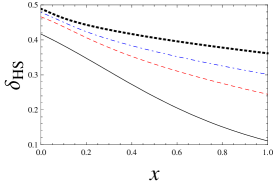
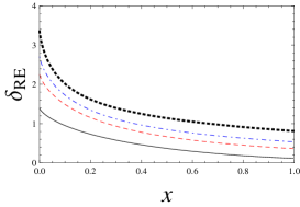
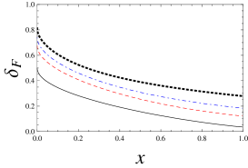
Figure 1: Dependence of the distance-type non-Gaussianity on the thermal parameter $x$ for $M$-photon-added thermal states with $M=1,3,5,10$ (from bottom to top).

The variation of non-Gaussianity with the number $M$ of added photons is shown in Fig. 2 for several values of the thermal mean occupancy.

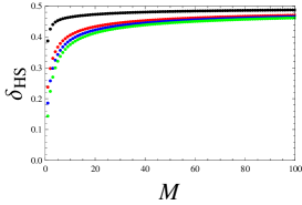
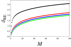
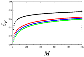
Figure 2: Dependence of the distance-type non-Gaussianity on the number of added photons. All the plots start from origin. We have used $\bar{n}=0.1,1,2,5$ (from top to bottom)

Besides showing a monotonic dependence on both parameters $\bar{n}$ and $M$, Figs. 1 and 2 seem to display a consistent relation between the three non-Gaussianity measures involved. To better outline this aspect and inspired by Ref.[11], we plot in Fig. 3 their mutual dependences when the parameter $x$ varies on its domain $x\in[0,1]$ at the same values of the number $M$ of added photons as in Fig.1. We can see that consistency is not present for all values of the parameters, especially in the dependence $\delta_{F}-\delta_{HS}$.

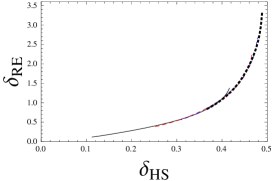
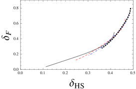
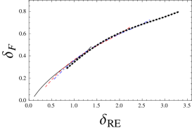
Figure 3: Mutual dependence of the distance-type non-Gaussianity measures  (LABEL:hsf), (2.18) and (2.19) for $M=1,3,5,10$ (from top to bottom). We have used $\bar{n}\in[0,1]$.

To conclude, in this paper we have introduced the Bures degree of non-Gaussianity built with Uhlmann’s fidelity between the given state and its associated Gaussian one. We have then investigated the behaviour of three distance-type measures of non-Gaussianity for an $M$-photon-added thermal state as functions of the variables $M$ and $\bar{n}$. We have found adequate monotonic dependences of $\delta_{HS}$, $\delta_{RE}$, and $\delta_{F}$ on both parameters $M$ and $\bar{n}$. This is displayed by Figs. 1 (as a function of the thermal mean occupancy) and 2 (as a function of the number of added photons). Although very different as geometric significance, the three measures seem to give consistent results by inducing the same ordering of non-Gaussianity. Figure 3 shows a very good consistency between $\delta_{RE}$ and $\delta_{HS}$ (left plot) and between $\delta_{F}$ and $\delta_{RE}$ (right plot). We also notice that the plots corresponding to different numbers $M$ of added photons are very close for all mutual dependences.

Appendix A Some useful formulae involving Gauss hypergeometric functions

A Gauss hypergeometric function is the sum of the corresponding hypergeometric series,

$${}_{2}F_{1}(a,b;c;z):=\sum\limits_{n=0}^{\infty}\frac{(a)_{n}(b)_{n}}{(c)_{n}}\frac{z^{n}}{n!}\,,\qquad(|z|<1),$$ (1.1)

where $(a)_{n}:=\Gamma(a+n)/\Gamma(a)$ is Pochhammer’s symbol. This definition is extended by analytic continuation [32]. Recall the linear transformation formula

$${}_{2}F_{1}(a,b;c;z)=(1-z)^{-b}\,{{}_{2}F_{1}}\left(c-a,b;c;\frac{z}{z-1}\right).$$ (1.2)

The Legendre polynomial of degree $M$ can be expressed in terms of a Gauss hypergeometric function:

$${\cal P}_{M}(z)={{}_{2}F_{1}}\left(-M,M+1;1;\frac{1-z}{2}\right),\qquad(M=0,1,2,3,...).$$ (1.3)

References

References

- [1] Dodonov V V 2002 J. Opt. B: Quantum Semiclass. Opt. 4 R1
- [2] Cahill K E 1969 Phys. Rev. 180 239
- [3] Hudson R L 1974 Rep. Math. Phys. 6 249
- [4] Kenfack A and Życzkowski K 2004 J. Opt. B: Quantum Semiclass. Opt. 6 396
- [5] Opatrný T, Kurizki G, and Welsch D -G 2000 Phys. Rev. A 61 032302
- [6] Olivares S, Paris M G A, and Bonifacio R 2003 Phys. Rev. A 67 032314
- [7] Dell’Anno F, De Siena S, Albano L, and Illuminati F 2007 Phys. Rev. A 76 022301
- [8] Cerf N J, Krüger O, Navez P, Werner R F, and Wolf M M 2005 Phys. Rev. Lett. 95 070501
- [9] Genoni M G, Paris M G A, and Banaszek K 2007 Phys. Rev. A 76 042327
- [10] Genoni M G, Paris M G A, and Banaszek K 2008 Phys. Rev. A 78 060303
- [11] Genoni M G and Paris M G A 2010 Phys. Rev. A 82 052341
- [12] Barbieri M et al. 2010 Phys. Rev. A 82 063833
- [13] Solomon I J, Sanjay K M, Simon R 2012 Quantum Inf. Process. 11 853
- [14] Uhlmann A 1976 Rep. Math. Phys. 9 273; 1986 Rep. Math. Phys. 24 229
- [15] Marian P, Marian T A, and Scutaru H 2002 Phys. Rev. Lett. 88 153601
- [16] Marian P, Marian T A, and Scutaru H 2003 Phys. Rev. A 68 062309
- [17] Marian P and Marian T A 2008 Phys. Rev. A 77 062319
- [18] Marian P and Marian T A 2008 Eur. Phys. J. Special Topics 160 281
- [19] Klimov A B, Sánchez-Soto L L, Yustas E C, Söderholm J, and Björk G 2005 Phys. Rev. A 72 033813
- [20] Sánchez-Soto L L, Yustas E C, Björk G, and Klimov A B 2007 Phys. Rev. A 76 043820
- [21] Luis A 2007 Opt. Commun. 273 173
- [22] Björk G, Söderholm J, Sánchez-Soto L L, Klimov A B, Ghiu I, Marian P, and Marian T A 2010 Opt. Commun. 283 4440
- [23] Ghiu I, Björk G, Marian P, and Marian T A 2010 Phys. Rev. A 82 023803
- [24] Bures D 1969 Trans. Am. Math. Soc. 135 199
- [25] Bengtsson I and Życzkowski K 2006 Geometry of Quantum States: An Introduction to Quantum Entanglement (Cambridge University Press, Cambridge, England)
- [26] Marian P and Marian T A 2012 Phys. Rev. A 86 022340
- [27] Agarwal G S and Tara K 1992 Phys. Rev. A 46 485
- [28] Jones G N, Haight J, and Lee C T 1997 Quantum Semiclass. Opt. 9 411
- [29] Zavatta A, Parigi V, and Bellini M 2007 Phys. Rev. A 75 052106
- [30] Kiesel T, Vogel W, Parigi V, Zavatta A, and Bellini M 2008 Phys. Rev. A 78 021804R
- [31] Kiesel T, Vogel W, Bellini M, and Zavatta A 2011 Phys. Rev. A 83 032116
- [32] Erdélyi A, Magnus W, Oberhettinger F and Tricomi F G 1953 Higher Transcendental Functions (New York:McGraw–Hill) Vol. 1