Group Model Selection Using Marginal Correlations:
The Good, the Bad and the Ugly

Abstract

Group model selection is the problem of determining a small subset of groups of predictors (e.g., the expression data of genes) that are responsible for majority of the variation in a response variable (e.g., the malignancy of a tumor). This paper focuses on group model selection in high-dimensional linear models, in which the number of predictors far exceeds the number of samples of the response variable. Existing works on high-dimensional group model selection either require the number of samples of the response variable to be significantly larger than the total number of predictors contributing to the response or impose restrictive statistical priors on the predictors and/or nonzero regression coefficients. This paper provides comprehensive understanding of a low-complexity approach to group model selection that avoids some of these limitations. The proposed approach, termed Group Thresholding (GroTh), is based on thresholding of marginal correlations of groups of predictors with the response variable and is reminiscent of existing thresholding-based approaches in the literature. The most important contribution of the paper in this regard is relating the performance of GroTh to a polynomial-time verifiable property of the predictors for the general case of arbitrary (random or deterministic) predictors and arbitrary nonzero regression coefficients.

I Introduction

I-A Motivation and Background

One of the most fundamental of problems in statistical data analysis is to learn the relationship between the samples of a dependent or response variable (e.g., the malignancy of a tumor, the health of a network) and the samples of independent or predictor variables (e.g., the expression data of genes, the traffic data in the network). This problem was relatively easy in the data-starved world of yesteryears. We had $n$ samples and $p$ predictors, and our inability to observe too many variables meant that we lived in the “$n$ greater than or equal to $p$” world. Times have changed now. The data-rich world of today has enabled us to simultaneously observe an unprecedented number of variables per sample. It is nearly impossible in many of these instances to collect as many, or more, samples as the number of predictors. Imagine, for example, collecting hundreds of thousands of thyroid tumors in a clinical setting. The “$n$ smaller than $p$” world is no longer a theoretical construct in statistical data analysis. It has finally arrived; and it is here to stay.

This paper concerns statistical inference in the “$n$ smaller than $p$” setting for the case when the response variable depends linearly on the predictors. Mathematically, a model of this form can be expressed as

$$y_{i}=\sum_{j=1}^{p}x_{i,j}\beta^{0}_{j}+\varepsilon_{i},\ i=1,\dots,n.$$ (1)

Here, $y_{i}$ denotes the $i$-th sample of the response variable, $x_{i,j}$ denotes the $i$-th sample of the $j$-th predictor, $\varepsilon_{i}$ denotes the error in the model, and the parameters $\{\beta^{0}_{j}\}$ are called regression coefficients. This relationship between the samples of the response variable and those of the predictors can be expressed compactly in matrix-vector form as $\mathrm{y}=X\beta^{0}+\varepsilon$. The matrix $X$ in this form, termed the design matrix, is an $n\times p$ matrix whose $j$-th column comprises the $n$ samples of the $j$-th predictor. In tumor classification, for example, an entry in the response variable $\mathrm{y}$ could correspond to the malignancy (expressed as a numerical number) of a tumor sample, while the corresponding row in $X$ would correspond to the expression level of $p$ genes in that tumor sample.

The linear model $\mathrm{y}=X\beta^{0}+\varepsilon$, despite its mathematical simplicity, continues to make profound impacts in countless application areas [1]. Such models are used for various inferential purposes. In this paper, we focus on the problem of model selection in high-dimensional linear models, which involves determining a small subset of $p$ predictors that are responsible for majority (or all) of the variation in the response variable $\mathrm{y}$. High-dimensional model selection can be used to implicate a small number of genes in the development of cancerous tumors, identify a small number of genes that primarily affect prognosis of a disease, etc.

Algorithm 1 The Group Thresholding (GroTh) Algorithm for Group Model Selection

Input: An $n\times p$ design matrix $X$, response variable $y$, number of predictors per group $r$, and (group) model order $k$
Output: An estimate $\widehat{\mathcal{K}}\subset\{1,\dots,m\}$ of the true (group) model $\mathcal{K}$

  $f\leftarrow\begin{bmatrix}X_{1}&X_{2}&\dots&X_{m}\end{bmatrix}^{\mathrm{T}}y$ {Compute marginal correlations}

  $\big{(}\mathcal{I},\big{\{}\|f_{(j)}\|_{2}\big{\}}\big{)}\leftarrow\text{SORT}\Big{(}\Big{(}\big{\{}1,\dots,m\big{\}},\big{\{}\|f_{i}\|_{2}:=\|X_{i}^{\mathrm{T}}y\|_{2}\big{\}}\Big{)}\Big{)}$ {Sort groups of marginal correlations}

  $\widehat{\mathcal{K}}\leftarrow\mathcal{I}[1:k]$ {Select model via group thresholding}

I-B Group Model Selection and Our Contributions

There exist many applications in statistical model selection where the implication of a single predictor in the response variable implies presence of other related predictors in the true model. This happens, for instance, in the case of microarray data when the genes (predictors) share the same biological pathway [2]. In such situations, it is better to reformulate the problem of model selection in a “group” setting. Specifically, the response variable $\mathrm{y}=X\beta^{0}+\varepsilon$ in high-dimensional linear models in group settings can be best explained by a small number of groups of predictors:

$$\mathrm{y}=\sum_{i=1}^{m}X_{i}\beta_{i}^{0}+\varepsilon=\sum_{i\in\mathcal{K}}X_{i}\beta_{i}^{0}+\varepsilon,$$ (2)

where $X_{i}$, an $n\times p_{i}$ submatrix of $X$, denotes the $i$-th group of predictors, $\beta_{i}^{0}$ denotes the group of $p_{i}$ regression coefficients associated with the group of predictors $X_{i}$, and the set $\mathcal{K}:=\{1\leq i\leq m:\beta^{0}_{i}\not=0\}$ denotes the underlying true (group) model, corresponding to the $k:=|\mathcal{K}|\ll m$ groups of predictors that explain $\mathrm{y}$.

One of the main contributions of this paper is comprehensive understanding of a polynomial-time algorithm, which we term Group Thresholding (GroTh), that returns an estimate $\widehat{\mathcal{K}}$ of the true (group) model $\mathcal{K}$ for the general case of arbitrary (random or deterministic) design matrices and arbitrary nonzero regression coefficients. To this end, we make use of two computable geometric measures of group coherence of a design matrix—the worst-case group coherence $\mu_{X}^{g}$ and the average group coherence $\nu_{X}^{g}$—to provide a nonasymptotic analysis of GroTh (Algorithm 1). We in particular establish that if $X$ satisfies a verifiable group coherence property then, for all but a vanishingly small fraction of possible models $\mathcal{K}$, GroTh: ($i$) handles linear scaling of the total number of predictors contributing to the response, $\sum_{i\in\mathcal{K}}p_{i}=O(n)$, and ($ii$) returns indices of the groups of predictors whose contributions to the response, {$\|\beta_{i}^{0}\|_{2}\}_{i\in\mathcal{K}}$, are above a certain self-noise floor that is a function of both $\mu_{X}^{g}$ and $\|\beta^{0}\|_{2}$.

I-C Relationship to Previous Work

The basic idea of using grouped predictors for inference in linear models has been explored by various researchers in recent years. Some notable works in this direction in the “$n\ll p$” setting include [3, 4, 5, 6, 7, 8, 9]. Despite these inspiring results, more work needs to be done for high-dimensional group model selection. This is because the results reported in [3, 4, 5, 6, 7, 8, 9] do not guarantee linear scaling of the total number of predictors contributing to the response for the case of arbitrary design matrices and nonzero regression coefficients.

The work in this paper is also related to another body of work in statistics and signal processing literature that studies the high-dimensional linear model $\mathrm{y}=X\beta^{0}+\varepsilon$ for the restrictive case of $X$ having a Kronecker structure: $X:=A^{\mathrm{T}}\otimes I$ for some matrix $A$, where $\otimes$ denotes the Kronecker product. An incomplete list of works in this direction includes [10, 11, 12, 13, 14, 15, 16]. These restrictive works, however, also fail to guarantee linear scaling of the total number of predictors contributing to the response for the case of arbitrary nonzero regression coefficients.

Finally, note that the group model selection procedure studied in this paper is based on analyzing the marginal correlations, $X^{\mathrm{T}}\mathrm{y}$, of predictors with the response variable. Therefore, our work is algorithmically similar to the group thresholding approaches of [13, 14, 8]. The main appeal of such approaches is their low computational complexity of $O(np)$, which is much smaller than the typical computational complexity associated with other model selection procedures [17]. In addition to the scaling limitations of the total number of influential predictors discussed earlier, however, the works in [13, 14, 8] also incorrectly conclude that performance of thresholding-based approaches is inversely proportional to the dynamic range, $\frac{\max_{i\in\mathcal{K}}\|\beta_{i}^{0}\|_{2}}{\min_{i\in\mathcal{K}}\|\beta_{i}^{0}\|_{2}}$, of the nonzero groups of regression coefficients.

I-D Mathematical Convention

The predictors and the response variable are assumed to be real valued throughout the paper, with the understanding that extensions to a complex-valued setting can be carried out in a straightforward manner. Uppercase letters are reserved for matrices, while lowercase letters are used for both vectors and scalars. Constants that do not depend upon the problem parameters (such as $n$, $m$, $p$, and $k$) are denoted by $c_{0}$, $c_{1}$, etc. The notation $\left[\!\left[{q}\right]\!\right]$ for $q\in\mathbb{N}$ is a shorthand for the set $\{1,\dots,q\}$, while the notation $\overset{D}{=}$ signifies equality in distribution. The transpose operation is denoted by $(\cdot)^{\mathrm{T}}$ and the spectral norm of a matrix is denoted by $\|\cdot\|_{2}$. Finally, the $\ell_{p,q}$ norm of a vector $v^{\mathrm{T}}=\begin{bmatrix}v_{1}^{\mathrm{T}}&\dots&v_{m}^{\mathrm{T}}\end{bmatrix}$ with each $v_{i}\in\mathbb{R}^{r}$ is defined as $\|v\|_{p,q}:=\left(\sum_{i=1}^{m}\|v_{i}\|^{q}_{p}\right)^{1/q}$ for $p,q\in(0,\infty]$, where $\|\cdot\|_{p}$ denotes the usual $\ell_{p}$ norm. Note that $\|v\|_{p,\infty}\equiv\max_{i}\|v_{i}\|_{p}$ and $\|v\|_{p,q}\equiv\|v\|_{q}$ for $r=1$.

I-E Organization

In Section II, we mathematically formulate the problem of group model selection, rigorously define the notions of worst-case group coherence, average group coherence and the group coherence property, and state and discuss the main result of the paper. In Section III, we prove the main result of the paper. Finally, we present some numerical results in Section IV and conclude in Section V.

II Group Model Selection Using GroTh

II-A Problem Formulation

The object of attention in this paper is the high-dimensional linear model $y=X\beta^{0}+\varepsilon$ relating the response variable $y\in\mathbb{R}^{n}$ to the $p$ $(\gg n)$ predictors comprising the columns of the design matrix $X$. Since scalings of the columns of $X$ can be absorbed into the regression vector $\beta^{0}$, we assume without loss of generality that the columns of $X$ have unit $\ell_{2}$ norms. There are three simplifying assumptions we make in this paper that will be relaxed in a sequel to this work. First, the modeling error is zero, $\varepsilon=0$, and thus the response variable is exactly equal to a parsimonious linear combination of grouped predictors: $y=\sum_{i\in\mathcal{K}}X_{i}\beta^{0}_{i}$. Second, the groups of predictors $\{X_{i}\}_{i=1}^{m}$ are characterized by the same number of predictors per group: $X_{i}\in\mathbb{R}^{n\times r}$ with $r:=\tfrac{p}{m}\leq n$. Third, the groups of predictors $\{X_{i}\}_{i=1}^{m}$ are orthonormalized: $X_{i}^{\mathrm{T}}X_{i}=I$.

The main goal of this paper is characterization of the performance of a group model selection procedure, termed GroTh, that returns an estimate $\widehat{\mathcal{K}}$ of the true model $\mathcal{K}$ by sorting the groups of marginal correlations $f_{i}:=X_{i}^{\mathrm{T}}\mathrm{y}$ according to their $\ell_{2}$-norms, $\|f_{i}\|_{2}$, in descending order and setting $\widehat{\mathcal{K}}$ to be indices of the first $k$ sorted groups of marginal correlations (see Algorithm 1). Instead of focusing on the worst-case performance of GroTh, however, we seek to characterize its performance for an arbitrary (but fixed) set of nonzero (grouped) regression coefficients supported on most models. Specifically, we do not impose any statistical prior on the set of nonzero regression coefficients, while we assume that the true (group) model $\mathcal{K}:=\{i\in\left[\!\left[{m}\right]\!\right]:\beta_{i}^{0}\not=0\}$ is a uniformly random $k$-subset of $\left[\!\left[{m}\right]\!\right]$. Finally, the metrics of goodness we use in this paper are the false-discovery proportion (fdp) and the non-discovery proportion (ndp), defined as

$$\textsf{{fdp}}(\widehat{\mathcal{K}}):=\frac{|\widehat{\mathcal{K}}\setminus\mathcal{K}|}{|\widehat{\mathcal{K}}|}\quad\text{and}\quad\textsf{{ndp}}(\widehat{\mathcal{K}}):=\frac{|\mathcal{K}\setminus\widehat{\mathcal{K}}|}{|\mathcal{K}|},$$ (3)

respectively. These two metrics have gained widespread usage in multiple hypotheses testing problems in recent years. In particular, the expectation of the fdp is the well-known false-discovery rate (fdr) [18, 19].

II-B Main Result and Discussion

Heuristically, successful group model selection requires the groups of predictors contributing to the response variable to be sufficiently distinguishable from the ones outside the true model. In this paper, we capture the notion of distinguishability of predictors through two easily computable, global geometric measures of the design matrix, namely, the worst-case group coherence and the average group coherence. The worst-case group coherence of $X$ is defined as

$$\mu_{X}^{g}:=\max_{i,j\in\left[\!\left[{m}\right]\!\right]:i\not=j}\|X_{i}^{\mathrm{T}}X_{j}\|_{2},$$ (4)

while the average group coherence of $X$ is defined as

$$\nu_{X}^{g}:=\frac{1}{m-1}\max_{i\in\left[\!\left[{m}\right]\!\right]}\Big{\|}\sum_{j\in\left[\!\left[{m}\right]\!\right]:j\not=i}X_{i}^{\mathrm{T}}X_{j}\Big{\|}_{2}.$$ (5)

Note that $\mu_{X}^{g}$ is a trivial upper bound on $\nu_{X}^{g}$. It is also worth pointing that the worst-case group coherence and its variants have existed in earlier literature [7, 20], but the average group coherence is defined for the first time in here.

The central thesis of this paper is that group model selection using GroTh can be successful if these two measures of group coherence of $X$ are small enough. In particular, we address the question of how small should these two measures be in terms of the group coherence property.

Definition 1 (The Group Coherence Property).

The $n\times rm$ design matrix $X$ is said to satisfy the group coherence property if the following two conditions hold for some positive constants $c_{\mu}$ and $c_{\nu}$:

$$\mu_{X}^{g} \leq\frac{c_{\mu}}{\sqrt{\log{m}}}\quad\text{and}$$ (GroCP-1)

$$\nu_{X}^{g} \leq c_{\nu}\mu_{X}^{g}\sqrt{\frac{r\log{m}}{n}}.$$ (GroCP-2)

It is straightforward to observe from the above definition that the group coherence property is a global property of $X$ that can be explicitly verified in polynomial time. Finally, we define $\beta^{0}_{(\ell)}$ to be the $\ell$-th largest group of nonzero regression coefficients: $\|\beta^{0}_{(1)}\|_{2}\geq\|\beta^{0}_{(2)}\|_{2}\geq\dots\geq\|\beta^{0}_{(k)}\|_{2}>0$. We are now ready to state the main result of this paper.

Theorem 1 (Group Model Selection Using GroTh).

Suppose the design matrix $X$ satisfies the group coherence property with parameters $c_{\mu}$ and $c_{\nu}$. Next, fix parameters $c_{1}\geq 2$, $c_{2}\in(0,1)$, and define parameter $c_{3}:=\frac{32\sqrt{2e}(2c_{1}-1)}{(1-c_{2})(c_{1}-1)}$. Then, under the assumptions $c_{1}rk\leq n$, $c_{\mu}<c_{3}^{-1}$, and $c_{\nu}\leq\sqrt{c_{1}}c_{2}c_{3}$, we have with probability exceeding $1-e^{2}m^{-1}$ that

$$\Big{\{}i\in\mathcal{K}:\|\beta_{i}^{0}\|_{2}\geq c_{3}\mu_{X}^{g}\|\beta^{0}\|_{2}\sqrt{\log{m}}\Big{\}}\subset\widehat{\mathcal{K}},$$ (6)

resulting in $\textsf{{fdp}}(\widehat{\mathcal{K}})\leq 1-L/k$ and $\textsf{{ndp}}(\widehat{\mathcal{K}})\leq 1-L/k$, where $L$ is defined to be the largest integer for which the inequality $\|\beta_{(L)}^{0}\|_{2}\geq c_{3}\mu_{X}^{g}\|\beta^{0}\|_{2}\sqrt{\log{m}}$ holds. Here, the probability is with respect to the uniform distribution of the true model $\mathcal{K}$ over all possible models.

A proof of this theorem is given in Section III. We now provide a brief discussion of the significance of this result. First, Theorem 1 indicates that a polynomial-time verifiable property, namely, the group coherence property, of the design matrix can be checked to ascertain whether GroTh, which has computational complexity of $O(np)$, is well suited for group model selection. Second, it states that if $X$ satisfies the group coherence property then GroTh handles linear scaling of the total number of predictors contributing to the response, $rk=O(n)$, for all but a vanishingly small fraction $O(m^{-1})$ of models. This is in stark contrast to the earlier works [13, 14, 8] on thresholding-based approaches in high-dimensional linear models, which do not guarantee such linear scaling for the case of arbitrary nonzero regression coefficients. Note that while we do not provide in this paper explicit examples of design matrices satisfying the group coherence property, numerical results in Section IV show that the set of design matrices satisfying the group coherence property is not empty.

Finally, Theorem 1 offers a nice interpretation of the price one might have to pay in estimating the true model using only marginal correlations. Specifically, (6) in the theorem implies group thresholding of marginal correlations effectively gives rise to a self-noise floor of $O\left(\mu_{X}^{g}\|\beta^{0}\|_{2}\sqrt{\log{m}}\right)$. In words, the estimate $\widehat{\mathcal{K}}$ returned by GroTh is guaranteed to return the indices of all the groups of predictors whose contributions to the response variable (in the $\ell_{2}$ sense) are above the self-noise floor of $O\left(\mu_{X}^{g}\|\beta^{0}\|_{2}\sqrt{\log{m}}\right)$ (cf. 6). This is again a significant improvement over the earlier works [13, 14, 8], which suggest that performance of thresholding-based approaches is inversely proportional to the dynamic range, $\frac{\max_{i\in\mathcal{K}}\|\beta_{i}^{0}\|_{2}}{\min_{i\in\mathcal{K}}\|\beta_{i}^{0}\|_{2}}$, of the nonzero groups of regression coefficients. In order to expand on this, we observe from (6) that

$$\|\beta_{i}^{0}\|_{2} =\Omega\left(\mu_{X}^{g}\|\beta^{0}\|_{2}\sqrt{\log{m}}\right)$$

$$\Longleftrightarrow\quad\frac{\|\beta_{i}^{0}\|^{2}_{2}}{\|\beta^{0}\|^{2}_{2}/k} =\Omega\left(k\,(\mu_{X}^{g})^{2}\log{m}\right).$$ (7)

Theorem 1 and the left-hand side of (7) indicate that inclusion of the $i$-th group of predictors in the estimate $\widehat{\mathcal{K}}$ is in fact related to the ratio of the energy contributed by the $i$-th group of predictors to the average energy contributed per group of nonzero predictors: $\frac{\|\beta_{i}^{0}\|^{2}_{2}}{\|\beta^{0}\|^{2}_{2}/k}$. Further, this implies that an increase in the dynamic range that comes from a decrease in $\min_{i\in\mathcal{K}}\|\beta_{i}^{0}\|_{2}$ cannot affect the performance of GroTh too much since $\frac{\|\beta_{i}^{0}\|^{2}_{2}}{\|\beta^{0}\|^{2}_{2}/k}$ increases for most groups of predictors in this case. This is indeed confirmed by the numerical experiments reported in Section IV.

III Proof of the Main Result

We begin by developing some notation to facilitate the forthcoming analysis. Notice that the $p$-dimensional vector of marginal correlations, $f=X^{\mathrm{T}}y$, can be written as $m$ groups of $r$-dimensional marginal correlations: $f^{\mathrm{T}}=\begin{bmatrix}f_{1}^{\mathrm{T}}&\dots&f_{m}^{\mathrm{T}}\end{bmatrix}$ with the $r\times 1$ vector $f_{i}=X_{i}^{\mathrm{T}}y$. In the following, we use $X_{\mathcal{K}}$ (an $n\times rk$ submatrix of $X$), $\beta_{\mathcal{K}}^{0}$ (an $rk\times 1$ subvector of $\beta^{0}$), and $f_{\mathcal{K}}:=X_{\mathcal{K}}^{\mathrm{T}}y=X_{\mathcal{K}}^{\mathrm{T}}X_{\mathcal{K}}\beta_{\mathcal{K}}^{0}$ (an $rk\times 1$ subvector of $f$) to denote the groups of predictors, groups of regression coefficients, and the marginal correlations corresponding to the true model $\mathcal{K}$, respectively. Similarly, we use $X_{\mathcal{K}^{c}}$ and $f_{\mathcal{K}^{c}}:=X_{\mathcal{K}^{c}}^{\mathrm{T}}y=X_{\mathcal{K}^{c}}^{\mathrm{T}}X_{\mathcal{K}}\beta_{\mathcal{K}}^{0}$ to denote the groups of predictors and the marginal correlations corresponding to the complement set $\mathcal{K}^{c}:=\left[\!\left[{m}\right]\!\right]\setminus\mathcal{K}$, respectively.

III-A Lemmata

Proof of Theorem 1 requires understanding the behaviors of the $rk\times 1$ group vector $\big{(}X_{\mathcal{K}}^{\mathrm{T}}X_{\mathcal{K}}-I\big{)}\beta_{\mathcal{K}}^{0}$ and the $r(m-k)\times 1$ group vector $X_{\mathcal{K}^{c}}^{\mathrm{T}}X_{\mathcal{K}}\beta_{\mathcal{K}}^{0}$. In this subsection, we state and prove two lemmas that help us toward this goal. We will then leverage these two lemmas to provide a proof of Theorem 1.

Before proceeding, recall that $\mathcal{K}$ is taken to be a uniformly random $k$-subset of $\left[\!\left[{m}\right]\!\right]$, while the set of nonzero group regression coefficients $\{z_{i}\}_{i=1}^{k}:=\{\beta^{0}_{i}:i\in\mathcal{K}\}$ is considered to be deterministic (and fixed) but unknown. It therefore follows that the $rk$-dimensional group vector $\big{(}X_{\mathcal{K}}^{\mathrm{T}}X_{\mathcal{K}}-I\big{)}\beta_{\mathcal{K}}^{0}$ can be equivalently expressed as

$$\big{(}X_{\mathcal{K}}^{\mathrm{T}}X_{\mathcal{K}}-I\big{)}\beta_{\mathcal{K}}^{0}\overset{D}{=}\big{(}X_{\Pi}^{\mathrm{T}}X_{\Pi}-I\big{)}z,$$ (8)

where $\bar{\Pi}:=(\pi_{1},\dots,\pi_{m})$ is a random permutation of $\left[\!\left[{m}\right]\!\right]$, $\Pi:=(\pi_{1},\dots,\pi_{k})$ denotes the first $k$ elements of $\bar{\Pi}$, $X_{\Pi}:=\begin{bmatrix}X_{\pi_{1}}&\dots&X_{\pi_{k}}\end{bmatrix}$ is an $n\times rk$ submatrix of $X$, and $z^{\mathrm{T}}:=\begin{bmatrix}z_{1}^{\mathrm{T}}&\dots&z_{k}^{\mathrm{T}}\end{bmatrix}$ is an $rk\times 1$ (group) vector of nonzero regression coefficients. Similarly, the $r(m-k)$-dimensional group vector $X_{\mathcal{K}^{c}}^{\mathrm{T}}X_{\mathcal{K}}\beta_{\mathcal{K}}^{0}$ can be expressed as

$$X_{\mathcal{K}^{c}}^{\mathrm{T}}X_{\mathcal{K}}\beta_{\mathcal{K}}^{0}\overset{D}{=}X_{\Pi^{c}}^{\mathrm{T}}X_{\Pi}z$$ (9)

where $\Pi^{c}:=(\pi_{k+1},\dots,\pi_{m})$ denotes the last $m-k$ elements of $\bar{\Pi}$ and $X_{\Pi^{c}}:=\begin{bmatrix}X_{\pi_{k+1}}&\dots&X_{\pi_{m}}\end{bmatrix}$ is an $n\times r(m-k)$ submatrix of $X$.

Lemma 1.

Fix $c_{1}\geq 2$ and $\epsilon\in(0,1)$. Next, assume $k\leq\min\{\epsilon^{2}(\nu_{X}^{g})^{-2}+1,c_{1}^{-1}m\}$ and let $\Pi=(\pi_{1},\dots,\pi_{k})$ denote the first $k$ elements of a random permutation of $\left[\!\left[{m}\right]\!\right]$. Then for any fixed $rk\times 1$ group vector $z^{\mathrm{T}}:=\begin{bmatrix}z_{1}^{\mathrm{T}}&\dots&z_{k}^{\mathrm{T}}\end{bmatrix}$

$$\Pr\Big{(}\big{\|}\big{(}X_{\Pi}^{\mathrm{T}}X_{\Pi}-I\big{)}z\big{\|}_{2,\infty}\geq\epsilon\|z\|_{2}\Big{)}$$

$$\qquad\quad\leq e^{2}k\exp\Big{(}-c_{4}\big{(}\epsilon-\nu_{X}^{g}\sqrt{k-1}\big{)}^{2}(\mu_{X}^{g})^{-2}\Big{)},$$ (10)

where $c_{4}:=\frac{(c_{1}-1)^{2}}{1024e(2c_{1}-1)^{2}}$ is an absolute constant.

Proof.

The proof of this lemma relies heavily on Banach-space-valued Azuma’s inequality stated in the Appendix. To begin, note that

$$\|\left(X_{\Pi}^{\mathrm{T}}X_{\Pi}-I\right)z\|_{2,\infty}\equiv\max_{i\in\left[\!\left[{k}\right]\!\right]}\big{\|}\sum_{\begin{subarray}{c}j=1\\ j\not=i\end{subarray}}^{k}X_{\pi_{i}}^{\mathrm{T}}X_{\pi_{j}}z_{j}\big{\|}_{2}.$$ (11)

We next fix an $i\in\left[\!\left[{k}\right]\!\right]$ and define the event $\mathcal{A}_{i}^{\prime}:=\{\pi_{i}=i^{\prime}\}$ for $i^{\prime}\in\left[\!\left[{k}\right]\!\right]$. Then conditioned on $\mathcal{A}_{i}^{\prime}$, we have

$$\Pr\Big{(}\big{\|}\sum_{\begin{subarray}{c}j=1\\ j\not=i\end{subarray}}^{k}X_{\pi_{i}}^{\mathrm{T}}X_{\pi_{j}}z_{j}\big{\|}_{2}\geq\epsilon\|z\|_{2}\Big{|}\mathcal{A}_{i}^{\prime}\Big{)}$$

$$\qquad\qquad\quad=\Pr\Big{(}\big{\|}\sum_{\begin{subarray}{c}j=1\\ j\not=i\end{subarray}}^{k}X_{i^{\prime}}^{\mathrm{T}}X_{\pi_{j}}z_{j}\big{\|}_{2}\geq\epsilon\|z\|_{2}\Big{|}\mathcal{A}_{i}^{\prime}\Big{)}.$$ (12)

In order to make use of the concentration inequality in Proposition 1 in the Appendix for upper bounding (12), we construct an $\mathbb{R}^{r}$-valued Doob martingale on $\sum_{j\not=i}X_{i^{\prime}}^{\mathrm{T}}X_{\pi_{j}}z_{j}$. We first define $\Pi^{-i}:=(\pi_{1},\dots,\pi_{i-1},\pi_{i+1},\dots,\pi_{k})$ and then define the Doob martingale $(M_{0},M_{1},\dots,M_{k-1})$ as follows:

$$M_{0} :=\sum_{\begin{subarray}{c}j=1\\ j\not=i\end{subarray}}^{k}X_{i^{\prime}}^{\mathrm{T}}\mathbb{E}\big{[}X_{\pi_{j}}\big{|}\mathcal{A}_{i}^{\prime}\big{]}z_{j},\quad\text{and}$$

$$M_{\ell} =\sum_{\begin{subarray}{c}j=1\\ j\not=i\end{subarray}}^{k}X_{i^{\prime}}^{\mathrm{T}}\mathbb{E}\big{[}X_{\pi_{j}}\big{|}\pi_{1\rightarrow\ell}^{-i},\mathcal{A}_{i}^{\prime}\big{]}z_{j},\ \ell=1,\dots,k-1,$$

where $\pi_{1\rightarrow\ell}^{-i}$ denotes the first $\ell$ elements of $\Pi^{-i}$. The next step involves showing that the constructed martingale has bounded $\ell_{2}$ differences. In order for this, we use $\pi_{\ell}^{-i}$ to denote the $\ell$-th element of $\Pi^{-i}$ and define

$$M_{\ell}(u):=\sum_{\begin{subarray}{c}j=1\\ j\not=i\end{subarray}}^{k}X_{i^{\prime}}^{\mathrm{T}}\mathbb{E}\big{[}X_{\pi_{j}}\big{|}\pi_{1\rightarrow\ell-1}^{-i},\pi_{\ell}^{-i}=u,\mathcal{A}_{i}^{\prime}\big{]}z_{j}$$ (13)

for $u\in\left[\!\left[{m}\right]\!\right]$ and $\ell=1,\dots,k-1$. It can then be established using techniques very similar to the ones used in the method of bounded differences for scalar-valued martingales that [21, 22]

$$\|M_{\ell}-M_{\ell-1}\|_{2}\leq\sup_{u,v}\|M_{\ell}(u)-M_{\ell}(v)\|_{2}.$$ (14)

In order to upper bound $\|M_{\ell}(u)-M_{\ell}(v)\|_{2}$, we first define an $n\times r$ random matrix

$$\widetilde{X}_{\ell,j}^{u,v}:= \mathbb{E}\big{[}X_{\pi_{j}}\big{|}\pi_{1\rightarrow\ell-1}^{-i},\pi_{\ell}^{-i}=u,\mathcal{A}_{i}^{\prime}\big{]}$$

$$\qquad\qquad-\mathbb{E}\big{[}X_{\pi_{j}}\big{|}\pi_{1\rightarrow\ell-1}^{-i},\pi_{\ell}^{-i}=v,\mathcal{A}_{i}^{\prime}\big{]}.$$ (15)

Next, we notice that for every $j>\ell+1,j\not=i$, the random variable $\pi_{j}$ conditioned on $\{\pi_{1\rightarrow\ell-1}^{-i},\pi_{\ell}^{-i}=u,\mathcal{A}_{i}^{\prime}\}$ has a uniform distribution over $\left[\!\left[{m}\right]\!\right]\setminus\{\pi_{1\rightarrow\ell-1}^{-i},u,i^{\prime}\}$, while $\pi_{j}$ conditioned on $\{\pi_{1\rightarrow\ell-1}^{-i},\pi_{\ell}^{-i}=v,\mathcal{A}_{i}^{\prime}\}$ has a uniform distribution over $\left[\!\left[{m}\right]\!\right]\setminus\{\pi_{1\rightarrow\ell-1}^{-i},v,i^{\prime}\}$. Therefore, we get

$$\widetilde{X}_{\ell,j}^{u,v}=\frac{1}{m-\ell-1}\left(X_{u}-X_{v}\right),\quad j>\ell+1,j\not=i.$$ (16)

In order to evaluate $\widetilde{X}_{\ell,j}^{u,v}$ for $j\leq\ell+1,j\not=i$, we consider three cases for the index $i$. In the first case of $i\leq\ell$, it can be seen that $\widetilde{X}_{\ell,j}^{u,v}=0$ for every $j\leq\ell$ and $\widetilde{X}_{\ell,j}^{u,v}=X_{u}-X_{v}$ for $j=\ell+1$. In the second case of $i=\ell+1$, it can similarly be seen that $\widetilde{X}_{\ell,j}^{u,v}=0$ for every $j<\ell$ and $j=\ell+1$, while $\widetilde{X}_{\ell,j}^{u,v}=X_{u}-X_{v}$ for $j=\ell$. In the final case of $i>\ell+1$, it can be argued that $\widetilde{X}_{\ell,j}^{u,v}=0$ for every $j<\ell$, $\widetilde{X}_{\ell,j}^{u,v}=X_{u}-X_{v}$ for $j=\ell$, and $\widetilde{X}_{\ell,j}^{u,v}=\frac{1}{m-\ell-1}\left(X_{u}-X_{v}\right)$ for $j=\ell+1$. Consequently, regardless of the initial choice of $i$, we have

$$\|M_{\ell}(u)-M_{\ell}(v)\|_{2}$$

$$\quad\equiv\big{\|}\sum_{j\not=i}X_{i^{\prime}}^{\mathrm{T}}\widetilde{X}_{\ell,j}^{u,v}z_{j}\big{\|}_{2}\overset{(a)}{\leq}\sum_{\begin{subarray}{c}j\geq\ell\\ j\not=i\end{subarray}}\|X_{i^{\prime}}^{\mathrm{T}}\widetilde{X}_{\ell,j}^{u,v}\|_{2}\|z_{j}\|_{2}$$

$$\quad\overset{(b)}{\leq}2\mu_{X}^{g}\Big{(}\|z_{\ell}\|_{2}+\|z_{\ell+1}\|_{2}+\sum_{\begin{subarray}{c}j>\ell+1\\ j\not=i\end{subarray}}\frac{\|z_{j}\|_{2}}{m-\ell-1}\Big{)},$$ (17)

where $(a)$ is due to the triangle inequality and the submultiplicative nature of the induced norm, while $(b)$ primarily follows since $\|X_{i^{\prime}}^{\mathrm{T}}X_{u}-X_{i^{\prime}}^{\mathrm{T}}X_{v}\|_{2}\leq 2\mu_{X}^{g}$. We now have from (14) and (17) that $\|M_{\ell}-M_{\ell-1}\|_{2}\leq a_{\ell}$ with

$$a_{\ell}:=2\mu_{X}^{g}\Big{(}\|z_{\ell}\|_{2}+\|z_{\ell+1}\|_{2}+\sum_{\begin{subarray}{c}j>\ell+1\\ j\not=i\end{subarray}}\frac{\|z_{j}\|_{2}}{m-\ell-1}\Big{)}.$$ (18)

The next step needed to upper bound (12) involves providing an upper bound on $\|M_{0}\|_{2}$. To this end, note that

$$\|M_{0}\|_{2} \overset{(c)}{=}\big{\|}\sum_{j\not=i}X_{i^{\prime}}^{\mathrm{T}}\Big{(}\frac{1}{m-1}\sum_{\begin{subarray}{c}q=1\\ q\not=i^{\prime}\end{subarray}}^{m}X_{q}\Big{)}z_{j}\big{\|}_{2}$$

$$\leq\Big{\|}\frac{1}{m-1}\sum_{\begin{subarray}{c}q=1\\ q\not=i^{\prime}\end{subarray}}^{m}X_{i^{\prime}}^{\mathrm{T}}X_{q}\Big{\|}_{2}\Big{\|}\sum_{j\not=i}z_{j}\Big{\|}_{2}$$

$$\overset{(d)}{\leq}\nu_{X}^{g}\sum_{j\not=i}\|z_{j}\|_{2}\leq\nu_{X}^{g}\sqrt{k-1}\|z\|_{2},$$ (19)

where $(c)$ follows since $\pi_{j}$ conditioned on $\mathcal{A}_{i^{\prime}}$ has a uniform distribution over $\left[\!\left[{m}\right]\!\right]\setminus\{i^{\prime}\}$ and $(d)$ is a consequence of the definition of average group coherence. Finally, we note from [23, Lemma B.1] that $\rho_{\mathcal{B}}(\tau)$ defined in Proposition 1 satisfies $\rho_{\mathcal{B}}(\tau)\leq\tau^{2}/2$ for $(\mathcal{B},\|\cdot\|)\equiv(L_{2}(\mathbb{R}^{r}),\|\cdot\|_{2})$. Consequently, under the assumption that $k\leq\epsilon^{2}(\nu_{X}^{g})^{-2}+1$, it can be seen from our construction of the Doob martingale that

$$\Pr\Big{(}\big{\|}\sum_{\begin{subarray}{c}j=1\\ j\not=i\end{subarray}}^{k}X_{i^{\prime}}^{\mathrm{T}}X_{\pi_{j}}z_{j}\big{\|}_{2}\geq\epsilon\|z\|_{2}\Big{|}\mathcal{A}_{i}^{\prime}\Big{)}$$

$$\qquad\leq\Pr\Big{(}\big{\|}M_{k-1}-M_{0}\big{\|}_{2}\geq\big{(}\epsilon-\nu_{X}^{g}\sqrt{k-1}\big{)}\|z\|_{2}\Big{|}\mathcal{A}_{i}^{\prime}\Big{)}$$

$$\qquad\overset{(e)}{\leq}e^{2}\exp\Bigg{(}-\frac{c_{0}\big{(}\epsilon-\nu_{X}^{g}\sqrt{k-1}\big{)}^{2}\|z\|^{2}_{2}}{\sum\limits_{\ell=1}^{k-1}a_{\ell}^{2}}\Bigg{)},$$ (20)

where $(e)$ follows from Banach-space-valued Azuma’s inequality stated in the Appendix. Further, it can be established using (18) through tedious algebraic manipulations that

$$\sum_{\ell=1}^{k-1}a_{\ell}^{2} \leq\left(16+\frac{4k^{2}}{(m-k)^{2}}+\frac{16k}{m-k}\right)(\mu_{X}^{g})^{2}\|z\|^{2}_{2}$$

$$\overset{(f)}{\leq}4(2+(c_{1}-1)^{-1})^{2}(\mu_{X}^{g})^{2}\|z\|^{2}_{2},$$ (21)

where $(f)$ follows from the condition $k\leq m/c_{1}$. Combining all these facts together, we finally obtain from (20) and (21) the following concentration inequality:

$$\Pr\Big{(}\big{\|}\big{(}X_{\Pi}^{\mathrm{T}}X_{\Pi}-I\big{)}z\big{\|}_{2,\infty}\geq\epsilon\|z\|_{2}\Big{)}$$

$$\qquad\overset{(g)}{\leq}k\Pr\Big{(}\big{\|}\sum_{\begin{subarray}{c}j=1\\ j\not=i\end{subarray}}^{k}X_{\pi_{i}}^{\mathrm{T}}X_{\pi_{j}}z_{j}\big{\|}_{2}\geq\epsilon\|z\|_{2}\Big{)}$$

$$\qquad=k\sum_{i^{\prime}=1}^{m}\Pr\Big{(}\big{\|}\sum_{\begin{subarray}{c}j=1\\ j\not=i\end{subarray}}^{k}X_{i^{\prime}}^{\mathrm{T}}X_{\pi_{j}}z_{j}\big{\|}_{2}\geq\epsilon\|z\|_{2}\Big{|}\mathcal{A}_{i}^{\prime}\Big{)}\Pr(\mathcal{A}_{i}^{\prime})$$

$$\qquad\overset{(h)}{\leq}e^{2}k\exp\Big{(}-c_{2}\big{(}\epsilon-\nu_{X}^{g}\sqrt{k-1}\big{)}^{2}(\mu_{X}^{g})^{-2}\Big{)},$$ (22)

where $c_{4}:=c_{0}/4(2+(c_{1}-1)^{-1})^{2}$, $(g)$ follows from the union bound and the fact that $\pi_{i}$’s are identically distributed, while $(h)$ follows since $\pi_{i}$ has a uniform distribution over the set $\left[\!\left[{m}\right]\!\right]$. ∎

Lemma 2.

Fix $c_{1}\geq 2$ and $\epsilon\in(0,1)$. Next, assume $k\leq\min\{\epsilon^{2}(\nu_{X}^{g})^{-2},c_{1}^{-1}m\}$, and let $\Pi=(\pi_{1},\dots,\pi_{k})$ and $\Pi^{c}=(\pi_{k+1},\dots,\pi_{m})$ denote the first $k$ elements and the last $(m-k)$ elements of a random permutation of $\left[\!\left[{m}\right]\!\right]$, respectively. Then for any fixed $rk\times 1$ group vector $z^{\mathrm{T}}:=\begin{bmatrix}z_{1}^{\mathrm{T}}&\dots&z_{k}^{\mathrm{T}}\end{bmatrix}$

$$\Pr\Big{(}\big{\|}X_{\Pi^{c}}^{\mathrm{T}}X_{\Pi}z\big{\|}_{2,\infty}\geq\epsilon\|z\|_{2}\Big{)}$$

$$\quad\leq e^{2}(m-k)\exp\Big{(}-c_{5}\big{(}\epsilon-\nu_{X}^{g}\sqrt{k}\big{)}^{2}(\mu_{X}^{g})^{-2}\Big{)},$$ (23)

where $c_{5}:=\frac{(c_{1}-1)^{2}}{1024ec_{1}^{2}}$ is an absolute constant.

Proof.

The proof of this lemma is similar to that of Lemma 1 and also relies on Proposition 1 in the Appendix. To begin, we use $\pi_{i}^{c}$ to denote the $i$-th element of $\Pi^{c}$ and note

$$\|X_{\Pi^{c}}^{\mathrm{T}}X_{\Pi}z\|_{2,\infty}\equiv\max_{i\in\left[\!\left[{m-k}\right]\!\right]}\big{\|}\sum_{j=1}^{k}X_{\pi^{c}_{i}}^{\mathrm{T}}X_{\pi_{j}}z_{j}\big{\|}_{2}.$$ (24)

We next fix an $i\in\left[\!\left[{m-k}\right]\!\right]$ and define $\mathcal{A}_{i}^{\prime}:=\{\pi^{c}_{i}=i^{\prime}\}$ for $i^{\prime}\in\left[\!\left[{m-k}\right]\!\right]$. Then conditioned on $\mathcal{A}_{i}^{\prime}$, we again have the following simple equality:

$$\Pr\Big{(}\big{\|}\sum_{j=1}^{k}X_{\pi^{c}_{i}}^{\mathrm{T}}X_{\pi_{j}}z_{j}\big{\|}_{2}\geq\epsilon\|z\|_{2}\Big{|}\mathcal{A}_{i}^{\prime}\Big{)}$$

$$\qquad\qquad\quad=\Pr\Big{(}\big{\|}\sum_{j=1}^{k}X_{i^{\prime}}^{\mathrm{T}}X_{\pi_{j}}z_{j}\big{\|}_{2}\geq\epsilon\|z\|_{2}\Big{|}\mathcal{A}_{i}^{\prime}\Big{)}.$$ (25)

In order to upper bound (25) using Proposition 1, we now construct an $\mathbb{R}^{r}$-valued Doob martingale $(M_{0},M_{1},\dots,M_{k})$ on $\sum_{j}X_{i^{\prime}}^{\mathrm{T}}X_{\pi_{j}}z_{j}$ as follows:

$$M_{0} :=\sum_{j=1}^{k}X_{i^{\prime}}^{\mathrm{T}}\mathbb{E}\big{[}X_{\pi_{j}}\big{|}\mathcal{A}_{i}^{\prime}\big{]}z_{j},\quad\text{and}$$

$$M_{\ell} =\sum_{j=1}^{k}X_{i^{\prime}}^{\mathrm{T}}\mathbb{E}\big{[}X_{\pi_{j}}\big{|}\pi_{1\rightarrow\ell},\mathcal{A}_{i}^{\prime}\big{]}z_{j},\ \ell=1,\dots,k,$$

where $\pi_{1\rightarrow\ell}$ denotes the first $\ell$ elements of $\Pi$. The next step in the proof involves showing $\|M_{\ell}-M_{\ell-1}\|_{2}$ is bounded for all $\ell\in\left[\!\left[{k}\right]\!\right]$. To do this, we define

$$M_{\ell}(u)=\sum_{j=1}^{k}X_{i^{\prime}}^{\mathrm{T}}\mathbb{E}\big{[}X_{\pi_{j}}\big{|}\pi_{1\rightarrow\ell-1},\pi_{\ell}=u,\mathcal{A}_{i}^{\prime}\big{]}z_{j}$$ (26)

for $u\in\left[\!\left[{k}\right]\!\right]$ and once again resort to the argument in Lemma 1 that $\|M_{\ell}-M_{\ell-1}\|_{2}\leq\sup_{u,v}\|M_{\ell}(u)-M_{\ell}(v)\|_{2}$. Further, we define an $n\times r$ random matrix

$$\widetilde{X}_{\ell,j}^{u,v}:= \mathbb{E}\big{[}X_{\pi_{j}}\big{|}\pi_{1\rightarrow\ell-1},\pi_{\ell}=u,\mathcal{A}_{i}^{\prime}\big{]}$$

$$\qquad\qquad\quad-\mathbb{E}\big{[}X_{\pi_{j}}\big{|}\pi_{1\rightarrow\ell-1},\pi_{\ell}=v,\mathcal{A}_{i}^{\prime}\big{]}$$ (27)

and notice that $\widetilde{X}_{\ell,j}^{u,v}=0$ for $j<\ell$, $\widetilde{X}_{\ell,j}^{u,v}=X_{u}-X_{v}$ for $j=\ell$, and $\widetilde{X}_{\ell,j}^{u,v}=\frac{1}{m-\ell-1}(X_{u}-X_{v})$ for $j>\ell$. It then follows from this discussion that

$$\|M_{\ell}(u)-M_{\ell}(v)\|_{2} \leq\sum_{j=1}^{k}\|X_{i^{\prime}}^{\mathrm{T}}\widetilde{X}_{\ell,j}^{u,v}\|_{2}\|z_{j}\|_{2}$$

$$\overset{(a)}{\leq}2\mu_{X}^{g}\Big{(}\|z_{\ell}\|_{2}+\frac{\sum_{j>\ell}\|z_{j}\|_{2}}{m-\ell-1}\Big{)},$$ (28)

where $(a)$ is primarily due to $\|X_{i^{\prime}}^{\mathrm{T}}X_{u}-X_{i^{\prime}}^{\mathrm{T}}X_{v}\|_{2}\leq 2\mu_{X}^{g}$. We have now established that $\|M_{\ell}-M_{\ell-1}\|_{2}\leq a_{\ell}$ with

$$a_{\ell}:=2\mu_{X}^{g}\Big{(}\|z_{\ell}\|_{2}+\frac{\sum_{j>\ell}\|z_{j}\|_{2}}{m-\ell-1}\Big{)},\ \ell\in\left[\!\left[{k}\right]\!\right].$$ (29)

The final bound we need in order to utilize Proposition 1 is that on $\|M_{0}\|_{2}$. Similar to (19) in Lemma 1, however, it is straightforward to show that $\|M_{0}\|_{2}\leq\nu_{X}^{g}\sqrt{k}\|z\|_{2}$.

It now follows from our construction of the Doob martingale, Proposition 1 in the Appendix, [23, Lemma B.1] and the assumption $k\leq\epsilon^{2}(\nu_{X}^{g})^{-2}$ that

$$\Pr\Big{(}\big{\|}\sum_{j=1}^{k}X_{i^{\prime}}^{\mathrm{T}}X_{\pi_{j}}z_{j}\big{\|}_{2}\geq\epsilon\|z\|_{2}\Big{|}\mathcal{A}_{i}^{\prime}\Big{)}$$

$$\qquad\leq\Pr\Big{(}\big{\|}M_{k}-M_{0}\big{\|}_{2}\geq\big{(}\epsilon-\nu_{X}^{g}\sqrt{k}\big{)}\|z\|_{2}\Big{|}\mathcal{A}_{i}^{\prime}\Big{)}$$

$$\qquad\leq e^{2}\exp\Bigg{(}-\frac{c_{0}\big{(}\epsilon-\nu_{X}^{g}\sqrt{k}\big{)}^{2}\|z\|^{2}_{2}}{\sum\limits_{\ell=1}^{k}a_{\ell}^{2}}\Bigg{)}.$$ (30)

In addition, it can be shown using (29) and the assumption $k\leq m/c_{1}$ that $\sum_{\ell=1}^{k}a_{\ell}^{2}\leq 4(1+(c_{1}-1)^{-1})^{2}(\mu_{X}^{g})^{2}\|z\|^{2}_{2}$. Combining all these facts together, we obtain the claimed result as follows:

$$\Pr\Big{(}\big{\|}X_{\Pi^{c}}^{\mathrm{T}}X_{\Pi}z\big{\|}_{2,\infty}\geq\epsilon\|z\|_{2}\Big{)}$$

$$\overset{(b)}{\leq}(m-k)\Pr\Big{(}\big{\|}\sum_{j=1}^{k}X_{\pi^{c}_{i}}^{\mathrm{T}}X_{\pi_{j}}z_{j}\big{\|}_{2}\geq\epsilon\|z\|_{2}\Big{)}$$

$$=\!(m-k)\!\sum_{i^{\prime}=1}^{m}\Pr\Big{(}\big{\|}\sum_{j=1}^{k}X_{i^{\prime}}^{\mathrm{T}}X_{\pi_{j}}z_{j}\big{\|}_{2}\geq\epsilon\|z\|_{2}\Big{|}\mathcal{A}_{i}^{\prime}\Big{)}\Pr(\mathcal{A}_{i}^{\prime})$$

$$\overset{(c)}{\leq}e^{2}(m-k)\exp\Big{(}-c_{3}\big{(}\epsilon-\nu_{X}^{g}\sqrt{k}\big{)}^{2}(\mu_{X}^{g})^{-2}\Big{)},$$ (31)

where $c_{5}:=c_{0}/4(1+(c_{1}-1)^{-1})^{2}$, $(b)$ follows from the union bound and the fact that $\pi_{i}^{c}$’s are identically distributed, while $(c)$ follows since $\pi^{c}_{i}$ has a uniform distribution over the set $\left[\!\left[{m}\right]\!\right]$. ∎

​​	​​
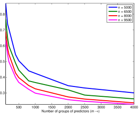
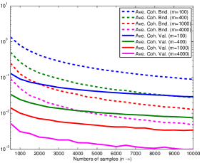
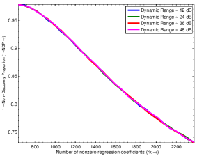
(a) Plots of $\mu_{X}^{g}\sqrt{\log{m}}$	(b) Plots of $\nu_{X}^{g}$ (solid) and $\mu_{X}^{g}\sqrt{r\log{m}/n}$ (dashed)	(c) Plots of $1-\textsf{{ndp}}$ for GroTh

Figure 1: Numerical experiments validating main result of the paper. Together, (a) and (b) illustrate that the set of design matrices satisfying the group coherence property is not empty. Further, (c) illustrates that the performance of GroTh is not exactly a function of the dynamic range $\frac{\max_{i\in\mathcal{K}}\|\beta_{i}^{0}\|_{2}}{\min_{i\in\mathcal{K}}\|\beta_{i}^{0}\|_{2}}$.

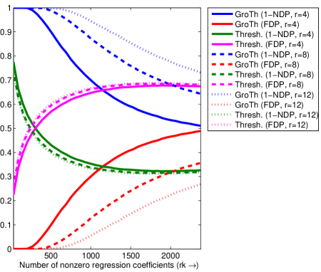
Figure 2: Comparison between the performances of GroTh and thresholding of individual marginal correlations that ignores the grouping of predictors.

III-B Proof of Theorem 1

Define $\widetilde{\mathcal{K}}:=\Big{\{}i\in\mathcal{K}:\|\beta_{i}^{0}\|_{2}\geq c_{3}\mu_{X}^{g}\|\beta^{0}\|_{2}\sqrt{\log{m}}\Big{\}}$. In order to prove this theorem, we need to understand the behavior of the marginal correlations corresponding to the restricted model $\widetilde{\mathcal{K}}$ and the marginal correlations corresponding to the complement set $\mathcal{K}^{c}$. To this end, recall the definition of $L$ from the statement of the theorem and note that

$$\min_{i\in\widetilde{\mathcal{K}}}\|f_{i}\|_{2} =\min_{i\in\widetilde{\mathcal{K}}}\|\beta_{i}^{0}+(X_{i}^{\mathrm{T}}X_{\mathcal{K}}\beta_{\mathcal{K}}^{0}-\beta_{i}^{0})\|_{2}$$

$$\geq\min_{i\in\widetilde{\mathcal{K}}}\|\beta_{i}^{0}\|_{2}-\max_{i\in\widetilde{\mathcal{K}}}\|(X_{i}^{\mathrm{T}}X_{\mathcal{K}}\beta_{\mathcal{K}}^{0}-\beta_{i}^{0})\|_{2}$$

$$=\|\beta_{(L)}^{0}\|_{2}-\|(X_{\mathcal{K}}^{\mathrm{T}}X_{\mathcal{K}}-I)\beta_{\mathcal{K}}^{0}\|_{2,\infty}.$$ (32)

In addition, we trivially have

$$\max_{i\in\mathcal{K}^{c}}\|f_{i}\|_{2}=\max_{i\in\mathcal{K}^{c}}\|X_{i}^{\mathrm{T}}X_{\mathcal{K}}\beta_{\mathcal{K}}^{0}\|_{2}=\|X_{\mathcal{K}^{c}}^{\mathrm{T}}X_{\mathcal{K}}\beta_{\mathcal{K}}^{0}\|_{2,\infty}.$$ (33)

It is easy to argue using (32) and (33) that

$$\|\beta_{(L)}^{0}\|_{2}>\|(X_{\mathcal{K}}^{\mathrm{T}}X_{\mathcal{K}}-I)\beta_{\mathcal{K}}^{0}\|_{2,\infty}+\|X_{\mathcal{K}^{c}}^{\mathrm{T}}X_{\mathcal{K}}\beta_{\mathcal{K}}^{0}\|_{2,\infty}$$ (34)

is a sufficient condition for the proof of the theorem. To see this, note that (34) implies $\min_{i\in\widetilde{\mathcal{K}}}\|f_{i}\|_{2}>\max_{i\in\mathcal{K}^{c}}\|f_{i}\|_{2}$. This in turn means $\widetilde{\mathcal{K}}\subset\widehat{\mathcal{K}}$, since $L\leq k$, resulting in $\textsf{{fdp}}(\widehat{\mathcal{K}})\leq 1-L/k$ and $\textsf{{ndp}}(\widehat{\mathcal{K}})\leq 1-L/k$.

The next step in the proof is therefore establishing that the sufficient condition (34) holds in our case. It is easy to show using Lemmas 1–2 and the union bound that

$$\|(X_{\mathcal{K}}^{\mathrm{T}}X_{\mathcal{K}}-I)\beta_{\mathcal{K}}^{0}\|_{2,\infty}+\|X_{\mathcal{K}^{c}}^{\mathrm{T}}X_{\mathcal{K}}\beta_{\mathcal{K}}^{0}\|_{2,\infty}\geq\epsilon\|\beta^{0}\|_{2}$$ (35)

with probability $\delta\leq e^{2}m\exp\Big{(}-c_{4}\big{(}\epsilon-\nu_{X}^{g}\sqrt{k}\big{)}^{2}(\mu_{X}^{g})^{-2}\Big{)}$ as long as $k\leq\min\{\epsilon^{2}(\nu_{X}^{g})^{-2},c_{1}^{-1}m\}$ for $c_{1}\geq 2$ and $\epsilon\in(0,1)$. We now fix $\epsilon=c_{3}\mu_{X}^{g}\sqrt{\log{m}}$ and claim that (35) holds with probability $\delta\leq e^{2}m^{-1}$ under the assumptions of the theorem. Notice that validity of this claim implies the sufficient condition (34) holds with probability $1-\delta\geq 1-e^{2}m^{-1}$ as long as $\|\beta_{(L)}^{0}\|_{2}\geq c_{3}\mu_{X}^{g}\|\beta^{0}\|_{2}\sqrt{\log{m}}$.

In order to complete the proof, we therefore need only establish the claim that (35) holds for $\epsilon=c_{3}\mu_{X}^{g}\sqrt{\log{m}}$ with probability $\delta\leq e^{2}m^{-1}$. In this regard, note: $(i)$ $\epsilon<1$ because of (GroCP-1) with $c_{\mu}<c_{3}^{-1}$ and $(ii)$ $\sqrt{k}\nu_{X}^{g}\leq c_{2}\epsilon$ because of $c_{1}rk\leq n$ and (GroCP-2) with $c_{\nu}\leq\sqrt{c_{1}}c_{2}c_{3}$. It then follows that (35) holds for $\epsilon=c_{3}\mu_{X}^{g}\sqrt{\log{m}}$ with probability $\delta\leq e^{2}m^{1-c_{4}(1-c_{2})^{2}c_{3}^{2}}$. The proof now trivially follows by noting that $c_{4}(1-c_{2})^{2}c_{3}^{2}=2$ for the chosen value of $c_{3}$. ∎

IV Numerical Results

In this section, we report the outcomes of some numerical experiments that validate Theorem 1. The $n\times p$ matrix $X$ in all these experiments is created as follows. First, we generate $m$ of $n\times r$ matrices $\widetilde{X}_{i}$ whose entries are drawn independently from a standard normal distribution. Next, we use the Gram–Schmidt process to orthonormalize $\widetilde{X}_{i}$’s and stack the resulting orthonormal $X_{i}$’s into an $n\times p$ design matrix $X$.

The first set of experiments reported in Fig. 1(a) and Fig. 1(b) confirms that the set of design matrices satisfying the group coherence property is not empty. Specifically, Fig. 1(a) plots $\mu_{X}^{g}\sqrt{\log{m}}$ as a function of $m$ for $p=20000$ and four different values of $n$. It can be seen from this figure that $\mu_{X}^{g}\sqrt{\log{m}}=O(1)$, which verifies (GroCP-1). Further, Fig. 1(b) plots both $\nu_{X}^{g}$ (solid lines) and $\mu_{X}^{g}\sqrt{r\log{m}/n}$ (dashed lines) as a function of $n$ for $p=20000$ and four different values of $m$. It can be seen from this figure that $\nu_{X}^{g}=O\big{(}\mu_{X}^{g}\sqrt{r\log{m}/n}\big{)}$, which verifies (GroCP-2).

The second set of experiments reported in Fig. 1(c) confirms that the performance of GroTh is not exactly a function of the dynamic range. In these experiments, corresponding to $p=15000$, $n=3000$ and $r=12$, all but one group of nonzero regression coefficients $\{\beta_{i}^{0}\}_{i\in\mathcal{K}}$ are normalized to have unit $\ell_{2}$ norms, while one randomly selected group of nonzero regression coefficients is normalized to yield specified dynamic range. Fig. 1(c) plots $1-\textsf{{ndp}}$ (averaged over $500$ random realizations of the true model $\mathcal{K}$) for GroTh under this setup as a function of $rk$ for four different values of dynamic range. It can be seen from this figure that the performance of GroTh indeed does not change with the dynamic range, because of the reasons outlined earlier in Section II.

The final set of experiments reported in Fig. 2 illustrates that GroTh performs better than thresholding of the individual marginal correlations that ignores the grouping of predictors. In these experiments, corresponding to $p=15000$ and $n=3000$, all groups of nonzero regression coefficients $\{\beta_{i}^{0}\}_{i\in\mathcal{K}}$ have unit $\ell_{2}$ norms, but individual nonzero regression coefficients do not necessarily have same magnitudes. Fig. 2 plots fdp and $1-\textsf{{ndp}}$ (averaged over $500$ random realizations of the true model $\mathcal{K}$) for both GroTh and (individual) thresholding under this setup as a function of $rk$ for three different values of $r$. It can be seen from this figure that thresholding of individual marginal correlations performs almost identically for different $r$. Performance of GroTh, on the other hand, improves with an increase in $r$.

V Conclusions

In this paper, we have provided a comprehensive understanding of Group Thresholding (GroTh) for high-dimensional group model selection. In particular, we have established that the performance of GroTh can be characterized in terms of a global geometric property of the design matrix that is explicitly verifiable in polynomial time. Results reported in this paper have also enhanced our understanding of thresholding-based approaches in high-dimensional linear models that rely on marginal correlations between the predictors and the response variable. In the future, we plan on extending this work by deriving fundamental bounds on worst-case and average group coherences, providing explicit examples of design matrices that satisfy the group coherence property, understanding the effects of modeling error, and relaxing the assumption of orthonormal groups of predictors.

[Banach-Space-Valued Azuma’s Inequality] In this appendix, we state a Banach-space-valued concentration inequality from [24] that is central to this paper.

Proposition 1 (Banach-Space-Valued Azuma’s Inequality).

Fix $s>0$ and assume that a Banach space $(\mathcal{B},\|\cdot\|)$ satisfies

$$\rho_{\mathcal{B}}(\tau):=\sup_{\begin{subarray}{c}u,v\in\mathcal{B}\\ \|u\|=\|v\|=1\end{subarray}}\left\{\frac{\|u+\tau v\|+\|u-\tau v\|}{2}-1\right\}\leq s\tau^{2}$$

for all $\tau>0$. Let $\{M_{k}\}_{k=0}^{\infty}$ be a $\mathcal{B}$-valued martingale satisfying the pointwise bound $\|M_{k}-M_{k-1}\|\leq a_{k}$ for all $k\in\mathbb{N}$, where $\{a_{k}\}_{k=1}^{\infty}$ is a sequence of positive numbers. Then for every $\delta>0$ and $k\in\mathbb{N}$, we have

$$\Pr\left(\|M_{k}-M_{0}\|\geq\delta\right)\leq e^{\max\{s,2\}}\exp\bigg{(}-\frac{c_{0}\delta^{2}}{\sum_{\ell=1}^{k}a_{\ell}^{2}}\bigg{)},$$

where $c_{0}:=\frac{e^{-1}}{256}$ is an absolute constant.

Remark 1.

Theorem 1.5 in [24] does not explicitly specify $c_{0}$ and also states the constant in front of $\exp(\cdot)$ to be $e^{s+2}$. Proposition 1 stated in its current form, however, can be obtained from the proof of Theorem 1.5 in [24].

References

- [1] A. C. Rencher and G. B. Schaalje, Linear Models in Statistics, 2nd ed. Hoboken, NJ: John Wiley & Sons, 2008.
- [2] M. R. Segal, K. D. Dahlquist, and B. R. Conklin, “Regression approaches for microarray data analysis,” J. Comput. Biol., vol. 10, no. 6, pp. 961–980, Jul. 2004.
- [3] M. Yuan and Y. Lin, “Model selection and estimation in regression with grouped variables,” J. Roy. Statist. Soc. Ser. B, vol. 68, no. 1, pp. 49–67, 2006.
- [4] F. Bach, “Consistency of the group lasso and multiple kernel learning,” J. Machine Learning Res., vol. 9, no. 6, pp. 1179–1225, Jun. 2008.
- [5] Y. Nardi and A. Rinaldo, “On the asymptotic properties of the group lasso estimator for linear models,” Electron. J. Stat., vol. 2, pp. 605–633, 2008.
- [6] J. Huang and T. Zhang, “The benefit of group sparsity,” Ann. Statist., vol. 38, no. 4, pp. 1978–2004, Aug. 2010.
- [7] Y. C. Eldar, P. Kuppinger, and H. Bölcksei, “Block-sparse signals: Uncertainty relations and efficient recovery,” IEEE Trans. Signal Processing, vol. 58, no. 6, pp. 3042–3054, Jun. 2010.
- [8] Z. Ben-Haim and Y. C. Eldar, “Near-oracle performance of greedy block-sparse estimation techniques from noisy measurements,” IEEE J. Select. Topics Signal Processing, vol. 5, no. 5, pp. 1032–1047, Sep. 2011.
- [9] E. Elhamifar and R. Vidal, “Block-sparse recovery via convex optimization,” IEEE Trans. Signal Processing, vol. 60, no. 8, pp. 4094–4107, Aug. 2012.
- [10] S. Cotter, B. Rao, K. Engan, and K. Kreutz-Delgado, “Sparse solutions to linear inverse problems with multiple measurement vectors,” IEEE Trans. Signal Processing, vol. 53, no. 7, pp. 2477–2488, Jul. 2005.
- [11] J. Tropp, A. Gilbert, and M. Strauss, “Algorithms for simultaneous sparse approximation. Part I: Greedy pursuit,” Signal Processing, vol. 86, no. 3, pp. 572–588, Apr. 2006.
- [12] J. Tropp, “Algorithms for simultaneous sparse approximation. Part II: Convex relaxation,” Signal Processing, vol. 86, no. 3, pp. 589–602, Apr. 2006.
- [13] R. Gribonval, H. Rauhut, K. Schnass, and P. Vandergheynst, “Atoms of all channels, unite! Average case analysis of multi-channel sparse recovery using greedy algorithms,” J. Fourier Anal. Appl., vol. 14, no. 5-6, pp. 655–687, Dec. 2008.
- [14] Y. C. Eldar and H. Rauhut, “Average case analysis of multichannel sparse recovery using convex relaxation,” IEEE Trans. Inform. Theory, vol. 56, no. 1, pp. 505–519, Jan. 2010.
- [15] G. Obozinski, M. Wainwright, and M. Jordan, “Support union recovery in high-dimensional multivariate regression,” Ann. Statist., vol. 39, no. 1, pp. 1–47, Jan. 2011.
- [16] M. Davies and Y. Eldar, “Rank awareness in joint sparse recovery,” IEEE Trans. Inform. Theory, vol. 58, no. 2, pp. 1135–1146, Feb. 2012.
- [17] J. Fan and J. Lv, “Sure independence screening for ultrahigh dimensional feature space [with comments, rejoinder],” J. Roy. Statist. Soc. Ser. B, vol. 70, no. 5, pp. 849–911, Nov. 2008.
- [18] Y. Benjamini and Y. Hochberg, “Controlling the false discovery rate: A practical and powerful approach to multiple testing,” J. Roy. Statist. Soc. Ser. B, vol. 57, no. 1, pp. 289–300, 1995.
- [19] F. Abramovich, Y. Benjamini, D. L. Donoho, and I. M. Johnstone, “Adapting to unknown sparsity by controlling the false discovery rate,” Ann. Statist., vol. 34, no. 2, pp. 584–653, 2006.
- [20] W. U. Bajwa, R. Calderbank, and M. F. Duarte, “On the conditioning of random block subdictionaries,” Department of Computer Science, Duke University, Technical Report TR-2010-06, Jun. 2010. [Online]. Available: http://www.rci.rutgers.edu/~wub1/pubs/TR2010_block_subdict.pdf
- [21] C. McDiarmid, “On the method of bounded differences,” in Surveys in Combinatorics, J. Siemons, Ed. Cambridge University Press, 1989, pp. 148–188.
- [22] R. Motwani and P. Raghavan, Randomized Algorithms. New York, NY: Cambridge University Press, 1995.
- [23] M. Donahue, C. Darken, L. Gurvits, and E. Sontag, “Rates of convex approximation in non-Hilbert spaces,” in Constructive Approximation. New York, NY: Springer, Jun. 1997, vol. 13, no. 2, pp. 187–220.
- [24] A. Naor, “On the Banach-space-valued Azuma inequality and small set isoperimetry of Alon–Roichman graphs,” Combinatorics, Probability and Computing, vol. 21, no. 04, pp. 623–634, Jul. 2012.