Learn with SAT to Minimize Büchi Automata

Abstract

We describe a minimization procedure for nondeterministic Büchi automata (NBA). For an automaton $A$ another automaton $A_{\min}$ with the minimal number of states is learned with the help of a SAT-solver.

This is done by successively computing automata $A^{\prime}$ that approximate $A$ in the sense that they accept a given finite set of positive examples and reject a given finite set of negative examples. In the course of the procedure these example sets are successively increased. Thus, our method can be seen as an instance of a generic learning algorithm based on a “minimally adequate teacher” in the sense of Angluin.

We use a SAT solver to find an NBA for given sets of positive and negative examples. We use complementation via construction of deterministic parity automata to check candidates computed in this manner for equivalence with $A$. Failure of equivalence yields new positive or negative examples. Our method proved successful on complete samplings of small automata and of quite some examples of bigger automata.

We successfully ran the minimization on over ten thousand automata with mostly up to ten states, including the complements of all possible automata with two states and alphabet size three and discuss results and runtimes; single examples had over 100 states.

1 Introduction

Minimization is a well-studied and widely used principle in many areas. In the theory of automata the best known example is the minimization of deterministic finite automata (DFA). It has the interesting property that by using only local optimizations one will always reach the same global minimum. This property is not valid anymore for some other automata models, nevertheless local optimization can still achieve a considerable reduction in size.

Because of that and its applications in automatic verification and other fields some incomplete minimization algorithms of nondeterministic Büchi automata (NBA) have been studied. They include local ([EH00] p. 6–11) minimizations, and other minimizations that do not guarantee to find a smallest automaton but only reduce the size [EF10]. Other studied minimization algorithms only work on some kind of Büchi automata (deterministic Büchi automata [Ehl10] or deterministic weak Büchi automata [Löd01]).

These algorithm try to balance computational efficiency with low size of the resulting NBA or with generality. After application of these algorithms it is not guaranteed that a found automaton is minimal nor can minimality of a given automaton be proven, or they are not applicable to all automata.

While this status is sufficient for many applications it is unsatisfactory not to have any algorithms for global minimization of NBA; on the theoretical side it is a gap, on the practical side it means that one never knows whether a given automaton might admit further reduction in size; especially when representing a policy the used automata are often very small and every additional state increases the resource consumption noticeable.

We present here the first procedure that computes for a given Büchi automaton an equivalent one of minimal size among all Büchi automata equivalent to the given one. We call this “global minimization for Büchi automata”.

Unlike in the case of deterministic finite automata such minimal automata are, however, not unique up to isomorphism.

Our approach can be seen as an instance of Angluin’s learning framework and indeed would be able to construct a minimal NBA for an arbitrary $\omega$-regular language presented by a minimally adequate teacher in the sense of [Ang87].

1.1 Büchi Automata

A nondeterministic Büchi automaton (NBA) describes a language of infinite words. It is given by a tuple $(Q,\Sigma,q_{0},F,\delta)$ where $Q$ is a finite set of states, $\Sigma$ a finite alphabet, $q_{0}\in Q$ the starting state, $F\subset Q$ the set of final states, and $\delta:Q\times\Sigma\rightarrow 2^{Q}$ the transition function. A word $a_{0}a_{1}a_{2}\dots\in\Sigma^{\omega}$ is said to be accepted if and only if $\exists q_{1}q_{2}q_{3}\dots$ such that $\forall i\in{\mathbb{N}}_{0}.q_{i+1}\in\delta(q_{i},a_{i})$ and $\forall i\in{\mathbb{N}}\,\exists j>i.q_{j}\in F$.

For example, a Büchi automaton for the language $L=(0|1)^{*}0^{\omega}$ (“finitely many 1s”) is shown in Figure 1

Figure 1: Example NBA, accepting the language $(0|1)^{*}0^{\omega}$

A run $q_{0}q_{1}q_{2}\dots$ on this automaton for a word $w\in L$ is obtained
by choosing $k\in{\mathbb{N}}.\forall l>k.w_{l}=0$ and setting $0=q_{0}=\dots=q_{k}$ and $1=q_{k+1}=\dots$

One defines the $\omega$-regular languages as those recognized by NBA.

1.2 Problem complexity

DFA can be minimized in polynomial time [Hop71] whereas minimization of deterministic Büchi automata is NP-complete [Sch10, Ehl10].

In case of NBA, the minimization problem is PSPACE-complete as it is already PSPACE-complete for nondeterministic finite automata ([Gra07] page 27, theorem 3) and it is easy to see that minimization of Büchi automata is in PSPACE given the well-known fact that equivalence of NBA is in PSPACE.

This in itself is not necessarily a problem because results of absolute minimization are nontrivial and of interest even for small problem instances. One may also remark that there exist practically and even industrially successful implementations of PSPACE hard problems, consider e.g. LTL model checking as implemented in the SPIN tool [Hol03] or even the WMSO implementation MONA [KM01].

The minimization procedure presented still leaves scope for further optimization, yet it is able to produce nontrivial and hitherto unknown results. For example, we were able to ascertain that in case of a two letter alphabet the complements of Büchi automata with two states require at most five states; we were also able to assert the minimality of the first instances of Michel’s family of NBA [Mic88], the first member of this family has two letters and two states and needs five states for its complement thus matching the here found limit for complement size for this automata size.

1.3 SAT solver

The abovementioned minimization algorithm of DBA [Ehl10] uses a SAT-solver to search for a DBA equivalent to a given one with a smaller number of states. To this end, equivalence of automata is encoded directly as a SAT formula which is possible since equivalence of DBA is in P. Since equivalence of NBA is PSPACE complete, this approach does not extend to NBA directly; nevertheless a SAT solver is a useful tool in our approach.

A SAT solver is a software that takes a boolean formula in conjunctive normal form (CNF) presented as a list of clauses in some machine readable format and returns a satisfying assignment if the formula is satisfiable and answers “unsatisfiable” otherwise.

Although satisfiability of CNF is NP-complete, modern SAT solvers can be applied to practically relevant and appreciably large instances. On modern computers, instances with 1000 variables and 10000 clauses are solvable in reasonable time. In specific cases even larger instances are solvable. This has earned SAT solvers a tremendous and still increasing popularity in recent years.

While the standard construction of CNF results in exponentially bigger formulas, introduction of fresh variables can limit this blowup to polynomial size.

2 Overview over the algorithm

The original automaton is transformed into a teacher for NBA in sense of Angluin [Ang87] by performing equivalence tests for constructing counterexamples or returning true.

The core is a candidate finder that creates Büchi automata out of positive (called good words) and negative (called bad words) word examples and additionally ensures minimal size for automata classifying these examples.

This is used to find candidates for the minimal automaton. A candidate is checked against the original automaton. In case of equivalence the candidate is a minimum automaton, whereas inequivality results in new good or bad words.

The candidate finder is presented in section 2.2, the algorithm using the learner as black box in section 2.3. Pseudo code presenting both at once is given in Figure 4.

2.1 Notation

The following notations are used in this paper:

• $w_{i}$ denotes the $i$-th letter of the word $w$.

• $[a]$ denotes the one-letter word consisting of $a\in\Sigma$;

• $i\,\,\frac{\enspace w\enspace}{\text{\enspace}}\!\!\!\!\!\scalebox{0.5}{\begin{tabular}[]{l}\vspace{0.9mm}\textgreater\vspace{0.9mm}\end{tabular}}\,j$ denotes a transition with the word $w$ from state $i$ to state $j$;

• $i\,\,\frac{\enspace w\enspace}{\enspace\text{F}\enspace}\!\!\!\!\!\scalebox{0.5}{\begin{tabular}[]{l}\vspace{0.9mm}\textgreater\vspace{0.9mm}\end{tabular}}\,j$ denotes a transition with the word $w$ from state $i$ to state $j$ with a visit of a final state anywhere on this path (including $i$ and $j$);

• $i\,\,\frac{\enspace v\enspace}{\text{\enspace}}\!\!\!\!\!\scalebox{0.5}{\begin{tabular}[]{l}\vspace{0.9mm}\textgreater\vspace{0.9mm}\end{tabular}}\,j\,\,\frac{\enspace w\enspace}{\text{\enspace}}\!\!\!\!\!\scalebox{0.5}{\begin{tabular}[]{l}\vspace{0.9mm}\textgreater\vspace{0.9mm}\end{tabular}}\,k$ is short for $i\,\,\frac{\enspace v\enspace}{\text{\enspace}}\!\!\!\!\!\scalebox{0.5}{\begin{tabular}[]{l}\vspace{0.9mm}\textgreater\vspace{0.9mm}\end{tabular}}\,j\land j\,\,\frac{\enspace w\enspace}{\text{\enspace}}\!\!\!\!\!\scalebox{0.5}{\begin{tabular}[]{l}\vspace{0.9mm}\textgreater\vspace{0.9mm}\end{tabular}}\,k$;

• $i\,\,\frac{\enspace v\enspace}{\bullet}\!\!\!\!\!\scalebox{0.5}{\begin{tabular}[]{l}\vspace{0.9mm}\textgreater\vspace{0.9mm}\end{tabular}}\,j\,\,\frac{\enspace w\enspace}{\bullet}\!\!\!\!\!\scalebox{0.5}{\begin{tabular}[]{l}\vspace{0.9mm}\textgreater\vspace{0.9mm}\end{tabular}}\,k$ is short for $(i\,\,\frac{\enspace v\enspace}{\text{\enspace}}\!\!\!\!\!\scalebox{0.5}{\begin{tabular}[]{l}\vspace{0.9mm}\textgreater\vspace{0.9mm}\end{tabular}}\,j\land j\,\,\frac{\enspace w\enspace}{\enspace\text{F}\enspace}\!\!\!\!\!\scalebox{0.5}{\begin{tabular}[]{l}\vspace{0.9mm}\textgreater\vspace{0.9mm}\end{tabular}}\,k)\lor(i\,\,\frac{\enspace v\enspace}{\enspace\text{F}\enspace}\!\!\!\!\!\scalebox{0.5}{\begin{tabular}[]{l}\vspace{0.9mm}\textgreater\vspace{0.9mm}\end{tabular}}\,j\land j\,\,\frac{\enspace w\enspace}{\text{\enspace}}\!\!\!\!\!\scalebox{0.5}{\begin{tabular}[]{l}\vspace{0.9mm}\textgreater\vspace{0.9mm}\end{tabular}}\,k)$.

• For an automaton $A$ we denote the language of the automaton by $L(A)$.

2.2 Candidate finder for Büchi automata

The candidate finder generates from given finite sets $G$ and $B$ of ultimately periodic words and an integer value $n$ a SAT formula whose satisfying assignments precisely correspond to automata $A^{\prime}$ with $n$ states such that $G\subseteq L(A^{\prime})\subseteq\overline{B}$.

The SAT formula represents an unknown automaton $X$ with $n$ states using variables $t_{i,j,a}$ (an $a$-labelled edge from $i$ to $j$) and $f_{i}$ (finality of state $i$). Further variables are defined, including $z_{u,v}$ ($uv^{\omega}$ is accepted by $X$). The formula itself then has to ensure these intended meanings and additionally comprises the conjunction of $z_{u,v}$ for $uv^{\omega}\in G$ and $\neg z_{u,v}$ for $uv^{\omega}\in B$.

variable	meaning
$f_{i}$	State $i$ is final state
$t_{i,j,a}$	$i\,\,\frac{\enspace[a]\enspace}{\text{\enspace}}\!\!\!\!\!\scalebox{0.5}{\begin{tabular}[]{l}\vspace{0.9mm}\textgreater\vspace{0.9mm}\end{tabular}}\,j$
$d_{i,j,w}$	$i\,\,\frac{\enspace w\enspace}{\text{\enspace}}\!\!\!\!\!\scalebox{0.5}{\begin{tabular}[]{l}\vspace{0.9mm}\textgreater\vspace{0.9mm}\end{tabular}}\,j$
$o_{i,j,k,a,w}$	$i\,\,\frac{\enspace[a]\enspace}{\text{\enspace}}\!\!\!\!\!\scalebox{0.5}{\begin{tabular}[]{l}\vspace{0.9mm}\textgreater\vspace{0.9mm}\end{tabular}}\,j\,\,\frac{\enspace w\enspace}{\text{\enspace}}\!\!\!\!\!\scalebox{0.5}{\begin{tabular}[]{l}\vspace{0.9mm}\textgreater\vspace{0.9mm}\end{tabular}}\,k$
$x_{w,i,j,m}$	There is a $k\in\{1,\dots,2^{m}\}$, such that $i\,\,\frac{\enspace w^{k}\enspace}{\text{\enspace}}\!\!\!\!\!\scalebox{0.5}{\begin{tabular}[]{l}\vspace{0.9mm}\textgreater\vspace{0.9mm}\end{tabular}}\,j$
$h_{w,i,j,k,m}$	There are $l_{1},l_{2}\in\{1,\dots,2^{m}\}$, such that $i\,\,\frac{\enspace w^{l_{1}}\enspace}{\text{\enspace}}\!\!\!\!\!\scalebox{0.5}{\begin{tabular}[]{l}\vspace{0.9mm}\textgreater\vspace{0.9mm}\end{tabular}}\,j\,\,\frac{\enspace w^{l_{2}}\enspace}{\text{\enspace}}\!\!\!\!\!\scalebox{0.5}{\begin{tabular}[]{l}\vspace{0.9mm}\textgreater\vspace{0.9mm}\end{tabular}}\,k$
$D_{i,j,w}$	$i\,\,\frac{\enspace w\enspace}{\enspace\text{F}\enspace}\!\!\!\!\!\scalebox{0.5}{\begin{tabular}[]{l}\vspace{0.9mm}\textgreater\vspace{0.9mm}\end{tabular}}\,j$
$O_{i,j,k,a,w}$	$i\,\,\frac{\enspace[a]\enspace}{\bullet}\!\!\!\!\!\scalebox{0.5}{\begin{tabular}[]{l}\vspace{0.9mm}\textgreater\vspace{0.9mm}\end{tabular}}\,j\,\,\frac{\enspace w\enspace}{\bullet}\!\!\!\!\!\scalebox{0.5}{\begin{tabular}[]{l}\vspace{0.9mm}\textgreater\vspace{0.9mm}\end{tabular}}\,k$
$s_{u,v,i,m}$	There is a $k\in\{1,\dots,2^{m}\}$ that $q\,\,\frac{\enspace uv^{k}\enspace}{\text{\enspace}}\!\!\!\!\!\scalebox{0.5}{\begin{tabular}[]{l}\vspace{0.9mm}\textgreater\vspace{0.9mm}\end{tabular}}\,i$
$u_{u,v,i,j,m}$	There is a $k\in\{1,\dots,{2^{m}}\}$ that $q\,\,\frac{\enspace u\enspace}{\text{\enspace}}\!\!\!\!\!\scalebox{0.5}{\begin{tabular}[]{l}\vspace{0.9mm}\textgreater\vspace{0.9mm}\end{tabular}}\,i\,\,\frac{\enspace v^{k}\enspace}{\text{\enspace}}\!\!\!\!\!\scalebox{0.5}{\begin{tabular}[]{l}\vspace{0.9mm}\textgreater\vspace{0.9mm}\end{tabular}}\,j$
$B_{i,j,w,m}$	There is a number $k\in\{1,\dots,2^{m}\}$ such that $i\,\,\frac{\enspace w\enspace}{\enspace\text{F}\enspace}\!\!\!\!\!\scalebox{0.5}{\begin{tabular}[]{l}\vspace{0.9mm}\textgreater\vspace{0.9mm}\end{tabular}}\,j\land j\,\,\frac{\enspace w^{k}\enspace}{\text{\enspace}}\!\!\!\!\!\scalebox{0.5}{\begin{tabular}[]{l}\vspace{0.9mm}\textgreater\vspace{0.9mm}\end{tabular}}\,i$
$L_{i,w,m}$	There is a number $k\in\{1,\dots,2^{m}\}$ and a state $j$ such that $i\,\,\frac{\enspace w\enspace}{\enspace\text{F}\enspace}\!\!\!\!\!\scalebox{0.5}{\begin{tabular}[]{l}\vspace{0.9mm}\textgreater\vspace{0.9mm}\end{tabular}}\,j\land j\,\,\frac{\enspace w^{k}\enspace}{\text{\enspace}}\!\!\!\!\!\scalebox{0.5}{\begin{tabular}[]{l}\vspace{0.9mm}\textgreater\vspace{0.9mm}\end{tabular}}\,i$
$y_{u,v,i}$	There are $k_{1},k_{2}\in\{1,\dots,2^{[\log_{2}(n)]+1}\}$ such that $q\,\,\frac{\enspace uv^{k_{1}}\enspace}{\text{\enspace}}\!\!\!\!\!\scalebox{0.5}{\begin{tabular}[]{l}\vspace{0.9mm}\textgreater\vspace{0.9mm}\end{tabular}}\,i\land i\,\,\frac{\enspace v^{k_{2}+1}\enspace}{\enspace\text{F}\enspace}\!\!\!\!\!\scalebox{0.5}{\begin{tabular}[]{l}\vspace{0.9mm}\textgreater\vspace{0.9mm}\end{tabular}}\,i$ (is $uv^{\omega}$ accepted via the state $i$ as loop knot).
$z_{u,v}$	The word $uv^{\omega}$ is accepted.

Table 1: Variables used in the SAT encoding

variable	deduction
$d_{i,j,\varepsilon}$	$i=j$
$d_{i,j,[a]}$	$t_{i,j,a}$
$d_{i,j,a.w}$	$\bigvee_{k=0\dots n-1}o_{i,j,k,a,w}$
$o_{i,j,k,a,w}$	$d_{i,k,[a]}\land d_{k,j,w}$
$x_{\varepsilon,i,j,m}$	$i=j$
$x_{w,i,j,0}$	$d_{i,j,w}$
$x_{w,i,j,m}$	$x_{w,i,j,m-1}\lor\bigvee_{k=0\dots n-1}h_{w,i,k,j,m-1}$
$z_{u,v}$	$\bigvee_{k=0\dots n-1}y_{u,v,k}$

Table 2: Definition of variables (selection)

Table 1 summarises the variables used in the expression. The variables are chosen in a way that every variable can be deduced by a small (constant size or linear in count of states) SAT formula from other variables; this limits the blowup for generating a CNF to polynomial instead of exponential size. These deductions follow in a simple way from their meaning; for some variables these deductions are shown in Table 2.

All in all the SAT expression consists of linear many variables as function of the alphabet size, the number of good and bad words and the length of the good and bad words. There are cubic many as function of the size of the automaton searched for.

The external used variables of this expression are:

• $z_{"","0"}$ (acceptance of the word $0^{\omega}$),

• $z_{"","1"}$ (acceptance of the word $1^{\omega}$),

• $t_{0,0,^{\prime}0^{\prime}}$ (existence of transition with letter $0$ from state $0$ to state $0$),

• $t_{0,0,^{\prime}1^{\prime}}$ (existence of transition with letter $1$ from state $0$ to state $0$) and

• $f_{0}$ (finality of state $0$).

$(u_{"","1",0,0,1}\iff(d_{0,0,""}\land x_{"1",0,0,1}))\land(s_{"","1",0,1}\iff u_{"","1",0,0,1})\land(D_{0,0,"1"}\iff({\bf t_{0,0,^{\prime}1^{\prime}}}\land{\bf f_{0}}))\land(d_{0,0,"1"}\iff{\bf t_{0,0,^{\prime}1^{\prime}}})\land(x_{"1",0,0,0}\iff d_{0,0,"1"})\land(h_{"1",0,0,0,0}\iff x_{"1",0,0,0})\land(x_{"1",0,0,1}\iff(x_{"1",0,0,0}\lor h_{"1",0,0,0,0}))\land(B_{0,0,"1",1}\iff(D_{0,0,"1"}\land x_{"1",0,0,1}))\land(L_{0,"1",1}\iff B_{0,0,"1",1})\land(y_{"","1",0}\iff(s_{"","1",0,1}\land L_{0,"1",1}))\land({\bf z_{"","1"}}\iff y_{"","1",0})\land(d_{0,0,""})\land(u_{"","0",0,0,1}\iff(d_{0,0,""}\land x_{"0",0,0,1}))\land(s_{"","0",0,1}\iff u_{"","0",0,0,1})\land(D_{0,0,"0"}\iff({\bf t_{0,0,^{\prime}0^{\prime}}}\land{\bf f_{0}}))\land(d_{0,0,"0"}\iff{\bf t_{0,0,^{\prime}0^{\prime}}})\land(x_{"0",0,0,0}\iff d_{0,0,"0"})\land(h_{"0",0,0,0,0}\iff x_{"0",0,0,0})\land(x_{"0",0,0,1}\iff(x_{"0",0,0,0}\lor h_{"0",0,0,0,0}))\land(B_{0,0,"0",1}\iff(D_{0,0,"0"}\land x_{"0",0,0,1}))\land(L_{0,"0",1}\iff B_{0,0,"0",1})\land(y_{"","0",0}\iff(s_{"","0",0,1}\land L_{0,"0",1}))\land({\bf z_{"","0"}}\iff y_{"","0",0})\land({\bf z_{"","1"}})\land(\neg{\bf z_{"","0"}})$

Solution computed by Minisat:

$u_{"","1",0,0,1}$, $d_{0,0,""}$, $x_{"1",0,0,1}$, $s_{"","1",0,1}$, $D_{0,0,"1"}$, ${\bf t_{0,0,^{\prime}1^{\prime}}}$, ${\bf f_{0}}$, $d_{0,0,"1"}$, $x_{"1",0,0,0}$, $h_{"1",0,0,0,0}$, $B_{0,0,"1",1}$, $L_{0,"1",1}$, $y_{"","1",0}$, ${\bf z_{"","1"}}$, $\neg u_{"","0",0,0,1}$, $\neg x_{"0",0,0,1}$, $\neg s_{"","0",0,1}$, $\neg D_{0,0,"0"}$, $\neg{\bf t_{0,0,^{\prime}0^{\prime}}}$, $\neg d_{0,0,"0"}$, $\neg x_{"0",0,0,0}$, $\neg h_{"0",0,0,0,0}$, $\neg B_{0,0,"0",1}$, $\neg L_{0,"0",1}$, $\neg y_{"","0",0}$, $\neg{\bf z_{"","0"}}$

Figure 2: SAT expression for $G=\{1^{\omega}\}$, $B=\{0^{\omega}\}$, $n=1$ and its solution

For further illustration, we present in Figure 2 the entire expression corresponding to $G=\{1^{\omega}\}$ and $B=\{0^{\omega}\}$ and $n=1$ as well as its satisfying assignment computed by Minisat. For better readability the formula is presented not in CNF while it is in CNF in the implementation. The only needed transformation for creating CNF is resolving the equivalences (denoted by “$\iff$”) thus roughly doubling the size of the expression.

example words	resulting automaton	example words	resulting automaton
$G=\{1^{\omega}\}$ $B=\{0^{\omega}\}$		$G=\{0^{\omega},1^{\omega}\}$ $B=\{(01)^{\omega}\}$
$G=\{01^{\omega},10^{\omega}\}$ $B=\{0^{\omega},1^{\omega}\}$		$G=\{(01)^{\omega}\}$ $B=\{0^{\omega},1^{\omega}\}$

Table 3: Example calculations of candidate automata from sets of words

Table 3 shows some calculations of candidate automata from sets $G$ and $B$ obtained in this way. We remark that even though in the right column the sets $G$ and $B$ are swapped, the resulting automata are not complementary as for example neither automaton accepts $01^{\omega}$.

2.3 Minimization algorithm

This part describes the minimization algorithm; for a given automaton $A$ find an automaton $A_{\text{min}}$ such that $A_{\text{min}}$ is equivalent to $A$ and no automaton with fewer states is equivalent to $A$.

• Step 1: Choose sets of ultimately periodic words $G$ and $B$. One may use empty sets; any sets of words such that $G\subseteq L(A)\subseteq\overline{B}$ are adequate.

• Step 2: Use the candidate finder to gain some automaton $A^{\prime}$ out of $G$ and $B$ with minimal number of states such that $G\subseteq L(A^{\prime})\subseteq\overline{B}$.

• Step 3: If $L(A)=L(A^{\prime})$ then $A^{\prime}$ is returned as minimal automaton; in the opposing case choose some counterexample $uv^{\omega}$ and expand $G$ or $B$ with it. Now resume at step 2 with the bigger sets.

This algorithm terminates as the sets $G$ and $B$ hinder any automaton occured once to occur again. Furthermore there are only finitely many automata smaller than $A$ so after finitely many steps $A$ would be returned if no smaller equivalent automaton could be found.

Furthermore the automaton returned has to be equivalent to $A$ as this is checked before returning the automaton. It is furthermore minimal as no smaller automaton can separate $G$ and $B$ but every automaton equivalent to $A$ does so.

2.4 Implementation

We have implemented the algorithm in Ocaml, Minisat2 [ES] is used as SAT solver.

Figure 3 displays the main data flow while Figure 4 summarises the complete algorithm in pseudocode.

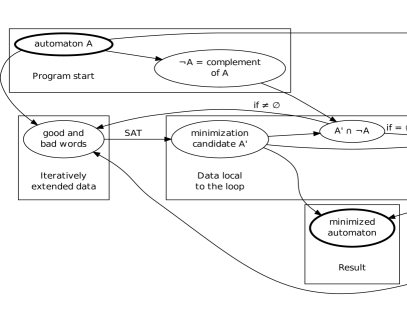
Figure 3: Main data flow for minimization

00:A = automaton to be minimized;
01:negA = complement A;
02:G = B = {}; (* Sets of good and bad words. *)
03:n = 1;
04:loop beginning
05:    try A’ = NBA-from-solution (SAT-solver (SAT-expression G B n))
06:       failure -> (* No automaton with n states could be found. *)
07:          n := n + 1;
08:          back to loop beginning;
09:       success -> (* A’ is candidate for minimized automaton. *)
10:          xB = intersect A’ negA;
11:          if xB nonempty
12:             B := B $\cup$ {onewordfrom xB}; (* new bad word. *)
13:             back to loop beginning;
14:          else (* L(A’) $\subseteq$ L(A) *)
15:             negA’ = complement A’;
16:             xG = intersect A negA’;
17:             if xG nonempty
18:                G := G $\cup$ {onewordfrom xG}; (* new good word. *)
19:                back to loop beginning;
20:             else (* L(A) $\subseteq$ L(A’) *)
21:                return A’.

Figure 4: Pseudo code for the complete algorithm

Calculating example words.

Counterexamples to $L(A)\stackrel{{\scriptstyle?}}{{=}}L(A^{\prime})$ are obtained as words in the language of NBA $B$ or $C$ which are constructed from $A$ and $A^{\prime}$ such that $L(B)=L(A)\backslash L(A^{\prime})$ and $L(C)=L(A^{\prime})\backslash L(A)$, thus finding a word in $L(B)$ or $L(C)$ results in a word in $L(B)\cup L(C)=L(A)\mathrel{\triangle}L(A^{\prime})$ where $\triangle$ denotes symmetric difference. We now describe how to decide whether for arbitrary NBA $D$ we have $L(D)\neq\emptyset$ and in the affirmative case how to construct an ultimately periodic word $uv^{\omega}\in L(D)$.

We begin by calculating the strongly connected components of $D$ by some linear algorithm, in our case Kosaraju’s algorithm [CC]. Subsequently, we choose a final state $i$ in a strongly connected component of size at least two or that has a transition to itself and can be reached from the starting state with some finite word $u$. There is a path from $i$ to $i$ with some nonempty word $v$ as $i$ has a transition to itself or lies in a strongly connected component of size at least two.

From this construction we then know that $uv^{\omega}\in L(D)$. We further try to reduce the lengths of $u$ and $v$ by favoring small strongly connected components that are close to the starting state and by further reducing the size of $u$ making use of the identity $xy(ly)^{\omega}=x(yl)^{\omega}$ where applicable.

Complementation.

To test for equivalence we need to repeatedly complement the candidate automata $A^{\prime}$ as well as the input automaton $A$ itself. Thus, complementation forms an important component of our algorithm and the choice of the right algorithm as well as its implementation will be crucial.

As suggested by [TFVT10] complementation of NBA by transforming them into deterministic parity automata (DPA), complementing them and transform them back to NBA is preferable. Thus this procedure is used here and leads indeed to small runtimes for that part of the algorithm. For transformation of NBA to DPA the algorithm of Safra enhanced by Piterman [Pit07] is used.

2.5 Optimizations

We used different optimization to improve the runtime of the algorithm.

Complement storage.

As the complement of the base automaton is used often we calculate it at the beginning and store it.

First search for bad words.

As this does not include complementation of an automaton it is more efficient to search for words in $\overline{A}\cap A^{\prime}$ and skip complementation of candidate automaton $A^{\prime}$ if a bad word could be found.

Size reduction of NBA.

We implemented a series of size reducing algorithms for NBA that require only linear runtime; they are applied on all intermediate automata and give a notable optimization of runtime. The used algorithm include

• Drop unreachable states

• Drop states where the automaton gets stuck

• Use a heuristic to detect some states from where all words are accepted. Merge them to one universal state and drop all outgoing transitions

• Drop transitions that could otherwise have been used to reach that universal state

Stop if no smaller automaton found.

If no smaller automaton was found we have proven minimality and can return the base automaton.

Choose start words.

For the needed sets of good and bad words some short (respective their representation) words are chosen. This does not only reduce the number of needed calls of the automaton finder but also reduces the runtime for the single calls of the SAT solver at least if there are not too many short words in it. How many example words are useful changes with the introduction of other optimizations and is adapted by benchmarks from time to time. Currently the words $a^{\omega}$, $ab^{\omega}$, $(ab)^{\omega}$, $a(ab)^{\omega}$ for all different letters $a$ and $b$ as well as $w^{\omega}$ (where $w$ contains every letter exactly once) are used.

Extra knowledge for the SAT expression.

We can gain some knowledge out of the automaton to minimize and include it into the SAT expression. For example if no word starts with the letter $a$ we know that there is no transition from the starting state to any states with label $a$.

Giving an order to the states does also gain some speed. This technique is known as symmetry breaking and is also used.

2.6 Asymptotic runtime

Let $\text{SAT}(n)$ be the runtime of a SAT solver on an input of at most $n$ variables and clauses. Let $C(n)$ be the time required to complement an NBA with at most $n$ states and $c(n)$ the size of this complement automaton.

The runtime of our minimiser on an automaton of size $N$ with minimal automaton of size $n$ whose complement has already been computed can then be summarised by:

$$O(I\cdot(c(n)\cdot N+n\cdot c(N)+C(n)+SAT(O(I\cdot n^{3}))))$$

where $I$ is the number of iterations of our algorithm. Obviously, $I=2^{O(n)}$, but in practice, $I$ is much smaller than this bound.

The factor $I$ in the $SAT$ expression comes from the linear dependency of the SAT formulas on the number of example words.

Additionally, if the complement of the input automaton is already known the runtime depends only linearly on the size of the automaton for different automata describing the same language.

3 Experimental results

As said in the previous chapter the runtime for minimization depends much more on the size of the found minimal automaton than on the size of the original automaton.

Most given runtimes were measured on the same machine; 2300 MHz, Quad-Core AMD Opteron(tm) Processor 8356; for each calculation one core was used. Vague given runtimes were calculated on slower machines.

If the minimal automaton is small enough and the complementation of the automaton is fast enough even large automata can be minimized; for example we could find some randomly generated automata with 40 to 100 states whose minimal equivalent automata of size up to 5 could be found in some minutes; to ensure that this is the merit of the minimizer we ensured that the heuristic pre-minimizer could not reduce the size of the original automaton.

$(G(q\lor FGp)\land G(r\lor FG\neg p))\lor Gq\lor Gp$

0 1 2 3 4 5 6 7 $\neg p$ $p$ $\neg p$ $p$ $\neg p$ $p$ $\neg p$ $p$ $\neg q$ $\neg q$ $q$ $q$ $\neg q$ $\neg q$ $q$ $q$ $\neg r$ $\neg r$ $\neg r$ $\neg r$ $r$ $r$ $r$ $r$

Figure 5: LTL formula together with its minimal automaton and the boolean value to alphabet translation table

Resulting size	count	average time	10%-decile	median	90%-decile time
1	245	$9.71\cdot 10^{-2}\,\text{s}$	$5.66\cdot 10^{-3}\,\text{s}$	$7.65\cdot 10^{-3}\,\text{s}$	$2.85\cdot 10^{-1}\,\text{s}$
2	179	$2.98\cdot 10^{-1}\,\text{s}$	$4.08\cdot 10^{-2}\,\text{s}$	$3.00\cdot 10^{-1}\,\text{s}$	$5.45\cdot 10^{-1}\,\text{s}$
3	76	$2.04\,\text{s}$	$1.50\cdot 10^{-1}\,\text{s}$	$1.96\,\text{s}$	$4.02\,\text{s}$
4	80	$9.82\,\text{s}$	$3.33\,\text{s}$	$9.13\,\text{s}$	$2.08\cdot 10^{1}\,\text{s}$
5	66	$4.30\cdot 10^{1}\,\text{s}$	$1.46\cdot 10^{1}\,\text{s}$	$3.78\cdot 10^{1}\,\text{s}$	$8.47\cdot 10^{1}\,\text{s}$
6	53	$7.77\cdot 10^{2}\,\text{s}$	$1.04\cdot 10^{2}\,\text{s}$	$2.96\cdot 10^{2}\,\text{s}$	$1.50\cdot 10^{3}\,\text{s}$
7	38	$7.61\cdot 10^{3}\,\text{s}$	$4.16\cdot 10^{2}\,\text{s}$	$3.14\cdot 10^{3}\,\text{s}$	$2.24\cdot 10^{4}\,\text{s}$
8	2	$2.01\cdot 10^{4}\,\text{s}$	$7.78\cdot 10^{3}\,\text{s}$	—	$3.24\cdot 10^{4}\,\text{s}$
Abnormal termination	199

Table 4: Measured minimization times for automata of starting size 10.

Furthermore we used a simple LTL to NBA translator that intentionaly does not optimize very well, just using our heuristic minimizer for the intermediate steps of the construction. Nevertheless we can minimize them if the minimal size is not too big. A formula (taken from [EF10]; details of the experimental evaluation, formula 1.22) that lead to an automaton of size 157 and could be minimized in half an hour is shown in Figure 5 together with its minimal automaton. Remark that [EF10] used a partial minimizer on an 8 state version of this automaton and only could find a 6 state automaton representing this formula; we could find a 5 state automaton without using a well pre-minimized NBA.

Speed measurement is given in Table 4. Random NBA with $10$ states and alphabet size two were generated. States are final with probability $0.5$; for every two states $i,j$ and letter $a$ there is a transition from $i$ to $j$ with probability $0.15$. If there are unreachable states or states from where no word can be accepted the automaton is skipped. Abnormal termination means out of memory or timeout (12h). When starting with 7-state automata the table looks similar but has no abnormal termination; it does not give additional information about the runtime and is hence skipped.

Table 5 shows the minimization results for complement automata of all automata with small size; as complementation can result in exponential blowup this needed minimizations of automata of bigger sizes.

$|\text{states}|$ / $|\Sigma|$ / #different automata	2/2/768	2/3/12288
#reducing to size 1	478	4404
#reducing to size 2	290	7884
#minimal complement size 1	372	2850
#minimal complement size 2	206	2754
#minimal complement size 3	134	3024
#minimal complement size 4	40	2429
#minimal complement size 5	16	1039
#minimal complement size 6	—	180
#minimal complement size 7	—	12

Table 5: Complete sampling of automata with small sizes

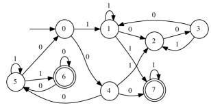
(a)	(c)

(b)

Figure 6: Automaton with 3 states and 2-letter-alphabet (a) with minimal complement size 8, its complement from the complementation (b) and its minimal complement automaton (c)

Having all these automata minimized one can now be sure that no automaton with two states and two letter alphabet needs more than 5 states for its complement. For three letter alphabet this limit is increased to 7 states. Only two (up to alphabet permutation) automata reach this limit.

Work is in progress to minimize all complements of automata with three states and two letter alphabet; an automaton with minimal complement of size 8 was found hereby; it is presented in Figure 6.

We also run our procedure on several instances of Michel’s automata $M_{n}$ over the alphabet $\Sigma=\{0,\dots,n\}$ and with $n+1$ states [Mic88] which were introduced to establish an $n!$ lower bound for complementation of NBA. Indeed, Michel has shown that no NBA with fewer than $n!$ states can recognize the complement of $L(M_{n})$.

The automata $M_{n}$ are given schematically on the left side in Figure 7 where $i$ represents a number in $\{1,\dots,n\}$, so $i\neq 0$.

Figure 7: Michel automaton schematically and minimal complement of $M_{1}$

We needed under a minute to compute the minimal complement of $M_{1}$; for $M_{2}$ we could prove that at least $7$ states are needed to represent it while the full minimization process timed out.

The minimality of $M_{n}$ for $1\leq n\leq 5$ could be proven as well.

Another calculated minimization example was taken from [EF10], a paper describing a minimization algorithm of NBA wherein a stronger form of equivalence, so-called bounded language equivalence, is used. It is presented in Figure 8. The automata shown are language equivalent, but not bounded language equivalent. As result a minimizer based on bounded language equivalence could not find (b) as minimal automaton for (a).

(a)	(b)	(minimized)

Figure 8: (a), (b): Automata shown in [EF10] page 15 Figure 5; alphabet was chosen with letter $0$ for $(\neg p,\neg r)$, $1$ for $(\neg p,r)$, $2$ for $(p,\neg r)$, $3$ for $(p,r)$; (minimized) is the result from our algorithm

Our complete minimizer could minimize the 6 state, 4 letter automaton (a) under a minute, leading to the result shown in Figure 8 (minimized). It did not find the automaton (b) from Figure 8, but instead another language equivalent but not bounded language equivalent automaton of the same size 5.

4 Conclusion

We have established the first global minimization algorithm for arbitrary nondeterministic Büchi automata. Previous algorithms were either restricted to special classes of Büchi automata or computed the automaton with the least number of states among those reachable from a given one by several optimization steps.

Despite the exponential worst-case running time of our algorithm we succeeded in applying it to several nontrivial automata with an acceptable runtime and in this way established previously unknown facts. Several people asked for a comparison with a naive brute force enumeration of all Büchi automata. We note here that already the number of automata with 5 states and alphabet size 2 exceeds $10^{16}$ and for every one of these a costly equivalence test would have to be performed which means that this procedure is infeasible for input automata with six or more states.

Of course, we did not establish a new upper bound of complexity with our algorithm but this was not to be expected as minimization of Büchi automata is PSPACE-complete. We also note that it has become common practice with good practical results to develop and use algorithms with exponential worst case runtime, e.g. SAT-solvers, or model checkers for LTL.

In particular we were able to assert that no Büchi automaton with two states and alphabet size two has a minimal complement automaton with more than five states and that the minimal complement automaton of Michel [Mic88] for alphabet size two achieves this bound. With the brute force enumeration such result would have been impossible to obtain even assuming some heuristic strategies to rule out candidates.

The implementation of the relatively straightforward optimizations described in Section 2.5 each produced considerable speedups; we thus hope that further relatively easy optimizations would allow us to push the limit of feasibility further out and make more applications accessible to our method. For all tested automata over a size of 4 for the minimal automaton over 50% of computational time went into the SAT-solver, most times over 99% of time is used here so further optimization focuses here.

We were asked to what extent our algorithm is able to produce certificates of the asserted minimality of its output. Since minimization is PSPACE complete we cannot in general expect polynomially sized certificates unless NP=PSPACE. However, we can remark here that the final sets of good ($G$) and bad words ($B$) together with the purported size $n$ of the minimal automaton can serve as a ceritificate of sorts in the following way. An opponent who is not convinced of the asserted result can first check that $G\subseteq L$ and $B\subseteq\overline{L}$ where $L$ is the language of the original automaton to be minimized. Thereafter, they could construct the SAT formula searching for an automaton of size $n-1$ whose language $L^{\prime}$ satisfies $G\subseteq L^{\prime}\subseteq\overline{B}$. Alternatively, we could provide a corresponding resolution proof. While potentially large and difficult to check, these certificates are considerably more concise and intuitively valid than the always-open fallback option of a complete trace of a run of the algorithm.

In particular, in automata-based software model checking [Hol03] one must check that all runs of a program are accepted by an often small policy automaton. Minimizing the latter might result in considerable gains if it is used repeatedly on many different programs. Consider e.g. that the automaton represents some publically advertised security policy or even a standard.

We also anticipate possible usages of our algorithm as a tool for research into Büchi automata and teaching thereof. It could for example be used to early refute hypotheses about the strength of minimization heuristics yet to be invented. Notice here that our algorithm was able to further minimize the automaton from [EF10].

Finally, it will also be interesting to apply our SAT-based search to other instances of “minimally adequate teachers” for $\omega$-regular languages, in particular the ones arising from compositional verification [CG11].

References

- [1]
- [Ang87] D. Angluin (1987): Learning Regular Sets from Queries and Counterexamples. Inf. Comput. 75(2), pp. 87–106. Available at http://dx.doi.org/10.1016/0890-5401(87)90052-6.
-
[CC]
M. C. Chu-Carroll: Algorithm of
Kosaraju.
http://scienceblogs.com/
goodmath/2007/10/computing_strongly_connected_c.php. Accessed 14 July 2011. - [CG11] S. Chaki & A. Gurfinkel (2011): Automated assume-guarantee reasoning for omega-regular systems and specifications. ISSE 7(2), pp. 131–139. Available at http://dx.doi.org/10.1007/s11334-011-0148-1.
- [EF10] Rüdiger Ehlers & Bernd Finkbeiner (2010): On the Virtue of Patience: Minimizing Büchi Automata. In Jaco van de Pol & Michael Weber, editors: SPIN, Lecture Notes in Computer Science 6349, Springer, pp. 129–145. Available at http://dx.doi.org/10.1007/978-3-642-16164-3_10.
- [EH00] Kousha Etessami & Gerard J. Holzmann (2000): Optimizing Büchi Automata. In Catuscia Palamidessi, editor: CONCUR, Lecture Notes in Computer Science 1877, Springer, pp. 153–167. Available at http://dx.doi.org/10.1007/3-540-44618-4_13.
- [Ehl10] Rüdiger Ehlers (2010): Minimising Deterministic Büchi Automata Precisely Using SAT Solving. In Ofer Strichman & Stefan Szeider, editors: SAT, Lecture Notes in Computer Science 6175, Springer, pp. 326–332. Available at http://dx.doi.org/10.1007/978-3-642-14186-7_28.
- [ES] N. Eén & N. Sörensson: Minisat. http://minisat.se/. Accessed 13 August 2011.
- [Gra07] Gregor Gramlich (2007): Über die algorithmische Komplexität regulärer Sprachen. Ph.D. thesis. Available at http://publikationen.ub.uni-frankfurt.de/volltexte/2007/4577/.
- [Hol03] Gerard Holzmann (2003): SPIN MODEL CHECKER, the: primer and reference manual, first edition. Addison-Wesley Professional.
- [Hop71] J Hopcroft (1971): An n log n algorithm for minimizing states in a finite automaton. Reproduction , pp. 189–196Available at http://oai.dtic.mil/oai/oai?verb=getRecord&metadataPrefix=html&identifier=AD0719398.
- [KM01] Nils Klarlund & Anders Møller (2001): MONA Version 1.4 User Manual. BRICS, Department of Computer Science, Aarhus University. Notes Series NS-01-1. Available from http://www.brics.dk/mona/. Revision of BRICS NS-98-3.
- [Löd01] C. Löding (2001): Efficient minimization of deterministic weak omega-automata. Inf. Process. Lett. 79(3), pp. 105–109. Available at http://dx.doi.org/10.1016/S0020-0190(00)00183-6.
- [Mic88] M. Michel (1988): Complementation is more difficult with automata on infinite words. CNET, Paris.
- [Pit07] Nir Piterman (2007): From Nondeterministic Büchi and Streett Automata to Deterministic Parity Automata. CoRR abs/0705.2205. Available at http://arxiv.org/abs/0705.2205.
- [Sch10] Sven Schewe (2010): Minimisation of Deterministic Parity and Buchi Automata and Relative Minimisation of Deterministic Finite Automata. CoRR abs/1007.1333. Available at http://arxiv.org/abs/1007.1333.
- [TFVT10] Ming-Hsien Tsai, Seth Fogarty, Moshe Y. Vardi & Yih-Kuen Tsay (2010): State of Büchi Complementation. In Michael Domaratzki & Kai Salomaa, editors: CIAA, Lecture Notes in Computer Science 6482, Springer, pp. 261–271. Available at http://dx.doi.org/10.1007/978-3-642-18098-9_28.