Divide knot presentation of sporadic knots of
Berge’s lens space surgery

Abstract

Divide knots and links, defined by A’Campo in the singularity theory of complex curves, is a method to present knots or links by real plane curves. The present paper is a continuation of the author’s previous result that every knot in the major subfamilies of Berge’s lens space surgery (i.e., knots yielding a lens space by Dehn surgery) is presented by an L-shaped curve as a divide knot. In the present paper, L-shaped curves are generalized and it is shown that every knot in the minor subfamilies, called sporadic examples, of Berge’s lens space surgery is presented by a generalized L-shaped curve as a divide knot. A formula on the surgery coefficients and the presentation is also generalized.

1 Introduction

If $r$ Dehn surgery on a knot $K$ in $S^{3}$ yields the lens space $L(p,q)$, we call the pair $(K,r)$ a lens space surgery, and we also say that $K$ admits a lens space surgery, and that $r$ is the coefficient of the lens space surgery. The task of classifying lens space surgeries, especially knots that admit lens space surgeries has been a focal point in low-dimensional topology. In 1990, Berge [Bg] pointed out a “mechanism” of known lens space surgery, that is, doubly-primitive knots in the Heegaard surface of genus $2$. Berge also gave a conjecturally complete list of such knots, described them by Osborne–Stevens’s “R-R diagrams” in [OS], and classified such knots into three families, and into 12 types in detail:

1. Knots in a solid torus (Berge–Gabai knots) : TypeI, II, … and VI (Berge [Bg2])

   Dehn surgery along a knot in a solid torus whose resulting manifold is also a solid torus. TypeI consists of torus knots. TypeII consists of $2$-cable of torus knots.

2. Knots in genus-one fiber surface : TypeVII and VIII (see Baker [Ba, Ba3] and also [Y1, Y5])

3. Sporadic examples (a), (b), (c) and (d) : TypeIX, X, XI and XII, respectively.

Their surgery coefficients are also decided. They are called Berge’s lens space surgeries. The numbering VII–XII (after VI) are used by Baker in [Ba2, Ba3]. It is conjectured by Gordon [G1, G2] that every knot of lens space surgery is a doubly-primitive knot.

In the present paper, we are concerned with the minor family (3). It is known that TypeIX and TypeXII (Berge’s (a) and (d)) are related, and that TypeX and TypeXI (Berge’s (b) and (c)) are related. Thus our targets are TypeIX and TypeX.

Notation 1.1

Throughout the paper, we let Type${\mathcal{X}}$ denote either TypeIX or TypeX, i.e., ${\mathcal{X}}=$ IX or X. Knots in Type $\mathcal{X}$ are parametrized by an integer $j$ with $j\not=0,-1$ ([Bg]), thus we call the knots $k_{IX}(j)$ for TypeIX, and $k_{X}(j)$ for TypeX, respectively. For the precise construction of the knots $k_{\mathcal{X}}(j)$, see Section 3.

Berge’s original classification (a)–(d) of sporadic examples in [Bg] was

(a)  $k_{IX}(j)$ with $j>0$,	(b)  $k_{X}(j)$ with $j>0$,
(c)  $k_{X}(j)!$ with $j<-1$,	(d)  $k_{IX}(j)!$ with $j<-1$,

respectively, see Deruelle–Miyaszaki–Motegi’s recent works [DMM, DMM2]. Table 1 is a list of some data of the knots $k_{\mathcal{X}}(j)$: the coefficients $p$ of their lens space surgeries of $k_{\mathcal{X}}(j)$, the second parameter $q$ of the resulting lens space $L(p,q)$ and the genus of $k_{\mathcal{X}}(j)$, which depends on the sign of $j$. Our convention about orientations of lens spaces is “$p/q$ Dehn surgery along an unknot is $-L(p,q)$”.

knot	$p$ ($=$ coefficient)	$q$ of $L(p,q)$	genus ($j>0$)	genus ($j<-1$)
$k_{IX}(j)$	$22j^{2}+9j+1$	$-(11j+2)^{2}$	$11j^{2}$	$11j^{2}+9j+2$
$k_{X}(j)$	$22j^{2}+13j+2$	$-(11j+3)^{2}$	$11j^{2}+2j$	$11j^{2}+11j+3$

Table 1: Data on Sporadic knots

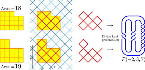
Figure 1: Divide knot presentation of $P(-2,3,7)$ (see [Y4, Y1])

The theory of A’Campo’s divide knots and links came from singularity theory of complex curves. A divide is originally a relative, generic immersion of a 1-manifold in the unit disk in $\mathbb{R}^{2}$, see Section 2. A’Campo [A1, A2, A3, A4] formulated the way to associate to each divide $P$ a link $L(P)$ in $S^{3}$. In the present paper, we regard a PL (piecewise linear) plane curve as a divide by smoothing the corners and controlling the size. Let $X$ be the $\pi/4$-lattice defined by $\{(x,y)|\cos\pi x=\cos\pi y\}$ in $xy$-plane. In this paper, we are interested in plane curves constructed as intersection of $X$ and a region. See Figure 1, which was the starting examples of the author’s project. Two L-shaped curves of the form $X\cap\mathcal{L}$ present a same knot, the pretzel knot of type $(-2,3,7)$, as divide knots. Its $18$-surgery and $19$-surgery are lens spaces (by Fintushel–Stern [FS]). Note that the areas of $\mathcal{L}$ are equal to the coefficients of the lens space surgeries. They have different mechanism of lens space surgeries: $18$-surgery is in TypeIII, $19$-surgery is in TypeVII.

Our question is

Question 1.2

Is every knot of (Berge’s) lens space surgeries a divide knot?

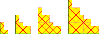
Case $j>0$ :  $P(1),P(2),P(3),P(4)$

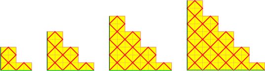
Case $j<-1$ :  $P(-2),P(-3),P(-4),P(-5)$

Figure 2: Plane curves $P(j)$, see Definition 3.1 for the precise definition

The purpose of the present paper is to give divide knot presentations of knots of sporadic examples. We show some plane curves to state the main results, see $P(j)$ in Figure 2. Each curve $P(j)$ is constructed as intersection of $X$ and a region that consists of some rectangles sharing the left bottom corner. We call such a curve a generalized L-shaped curve. The precise definition will be given in Section 2 and Section 3.

Next, we define plane curves $P_{\mathcal{X}}(j)$ from $P(j)$ by adding a square twice in the sense [Y4, Lemma 4.2].

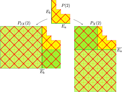
Figure 3: Add squares twice to get $P_{\mathcal{X}}(j)$  (ex. $P_{IX}(2)$ and $P_{X}(2)$)

Definition 1.3 (Plane curves $P_{\mathcal{X}}(j)$)

We let $E_{a}$ (and $E_{b}$, respectively) denote the bottom edge (and the left edge) of the region of $P(j)$, see Subsection 3.1 for the precise definition. For an integer $j$ with $j\not=0,-1$, depending on whether $\mathcal{X}=$ IX or X, we construct a region of $P_{\mathcal{X}}(j)$ as follows, see Figure 3.

1. [TypeIX]  We add a square along the bottom edge $E_{a}$ first, and add another square along the lengthened left edge $\overline{E_{b}}$.

2. [TypeX]  We add a square along the left edge $E_{b}$ first, and add another square along the lengthened bottom edge $\overline{E_{a}}$.

We remark that, by the first square addition along an edge $E_{a}$ (or $E_{b}$, respectively), the other edge $E_{b}$ (or $E_{a}$) is lengthened as $\overline{E_{b}}$ (or $\overline{E_{a}}$). The second square is added along the lengthened one. By $l(E)$ we denote the length of the edge $E$. Then,

$$l(E_{a})=|2j|,\ l(E_{b})=|2j+1|\text{ and }l(\overline{E_{b}})=l(\overline{E_{b}})=l(E_{a})+l(E_{b}).$$

Our main theorem is

Theorem 1.4

Up to mirror image, every knot in TypeIX and TypeX in Berge’s list of lens space surgery is a divide knot. More precisely, the plane curve $P_{\mathcal{X}}(j)$ presents the knot $k_{\mathcal{X}}(j)$ as a divide knot.

We will also show

Lemma 1.5

The plane curve $P(j)$ presents the torus knot $T(j,2j+1)$ as a divide knot.

Lemma 1.6

(see [DMM] on the knots)  We let $P_{m}(j)$ denote a plane curve obtained by a square addition along $E_{a}$ from $P(j)$, which appears in the process [TypeIX] to construct $P_{IX}(j)$ in Definition 1.3:

$$P(j)\ \rightarrow\ P_{m}(j)\ \rightarrow\ P_{IX}(j).$$

The plane curve $P_{m}(j)$ presents the cable knot $C(T(2,3);j,6j+1)$, regarded as $C(T(2,3);|j|,6|j|-1)$ if $j<-1$, of the trefoil as a divide knot:

$$T(j,2j+1)\ \rightarrow\ C(T(2,3);j,6j+1)\ \rightarrow\ k_{IX}(j).$$

The proof of Theorem 1.4 is divided into two parts: In the first half, starting with Baker’s Dehn surgery description in [Ba, Ba3], we study the knots by usual diagrams. In the second half, we will use divide presentations. We will introduce a convenient method, which we call Couture move, to deform generalized L-shaped curves. It was pointed out in the private communication of the author and Olivier Couture. With Couture moves, the proof get much geometric, intuitive and shorter. The author’s old proof of Theorem 1.4 was troublesome braid calculus. We will show Lemma 1.5 in the case $j<-1$ by Couture moves, as a demonstration, in Subsection 2.5.

On the relation between the surgery coefficient and the area of the region (of the curve), the formula in Theorem 1.4 in [Y4] is generalized to:

Lemma 1.7

On the divide presentation of $k_{\mathcal{X}}(j)$ by the generalized L-shaped curve $P_{\mathcal{X}}(j)$ in Theorem 1.4, the area, the number of concave points (of the region) of $P_{\mathcal{X}}(j)$ and the coefficient of the lens space surgery along $k_{\mathcal{X}}(j)$ satisfy

$$[\textrm{Area}-\sharp\{\textrm{Concave points}\}]-\textrm{Surgery coefficient}=0\textrm{ or }1.$$

see Definition 2.4 for the precise definition of concave points. Lemma 1.7 will be verified by Table 2 in Subsection 3.1.

Question 1.8

Study divide knots $L(P)$ presented by generalized L-shaped curves $P=X\cap\mathcal{L}$. By Lemma 1.7, $c(\mathcal{L})=\textrm{Area}(\mathcal{L})-\sharp\{\textrm{Concave points of }\mathcal{L}\}$ can be an expected coefficient for exceptional Dehn surgery of $L(P)$. Study $c(\mathcal{L})$ and $c(\mathcal{L})-1$ surgeries along $L(P)$.

This paper is organized as follows. In the next section, we review theory of A’Campo’s divide knots and links briefly and generalize L-shaped plane curve and decide the parametrizing notation. In Section 3, we review the construction of the knots $k_{\mathcal{X}}(j)$, give a precise definition of the plane curves $P(j)$ and prove Theorem 1.4 and the lemmas.

2 Divide knots and plane curves

We review theory of A’Campo’s divide knots and links briefly. We are interested in plane curves constructed as intersection of the $\pi/4$-lattice $X$ and a region. We define a generalized L-shaped plane curve and decide the parametrizing notation.

2.1 Torus knots

We start with a presentation of a (positive) torus knot as a divide knot. Let $(a,b)$ be a pair of positive integers and $B(a,b)$ a curve defined as an intersection of the $\pi/4$-lattice $X$ and an $a\times b$ rectangle $\mathcal{R}(a,b)$ whose every vertex is placed at a lattice point ($\in\mathbb{Z}^{2}$), see Figure 4. If $(a,b)$ is coprime, $B(a,b)$ is a billiard curve in $\mathcal{R}(a,b)$ with slope $\pm 1$.

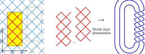
Figure 4: A billiard curve $B(a,b)$ presents a torus knot $T(a,b)$ (ex. $T(3,7)$)

Lemma 2.1

(Couture–Perron [CP], Goda–Hirasawa–Y [GHY], see also [AGV])
The curve $B(a,b)$ presents the torus link $T(a,b)$ as a divide knot.

Strictly, the curve $B(a,b)$ depends on the placement of the rectangle, whether the left-bottom corner of the region is a terminal of the curve or not, see Figure 4 again. Even if $(a,b)$ is not coprime (i.e., case of a torus link), the curve $B(a,b)$ in either choice presents $T(a,b)$ ([GHY]). If $(a,b)$ is coprime, the proof is easy: the reflection along $x$-axis maps one to the other.

2.2 Basic facts on divide knots

The theory of A’Campo’s divide knots and links comes from singularity theory of complex curves. A divide $P$ is (originally) a relative, generic immersion of a 1-manifold in the unit disk $D$ in $\mathbb{R}^{2}$. A’Campo [A1, A2, A3, A4] formulated the way to associate to each divide $P$ a link $L(P)$ in $S^{3}$. We regard $S^{3}$ as

$$S^{3}=\{(u,v)\in D\times T_{u}D\,|\,|u|^{2}+|v|^{2}=1\}$$

and the original construction is

$$L(P)=\{(u,v)\in D\times T_{u}D\,|\,u\in P,v\in T_{u}P,|u|^{2}+|v|^{2}=1\}\subset S^{3},$$

where $T_{u}P$ is the subset consisting of vectors tangent to $P$ in the tangent space $T_{u}D$ of $D$ at $u$. In the present paper, we regard a PL (piecewise linear) plane curve as a divide by smoothing corners and controlling the size.

Some characterizations of (general) divide knots and links are known, and some topological invariants of $L(P)$ can be gotten from the divide $P$ directly. Here, we list some of them.

Lemma 2.2

((1)–(7) by A’Campo [A2], (8) by Hirasawa [Hi], Rudolph [R])

1. $L(P)$ is a knot (i.e., connected) if and only if $P$ is an immersed arc.

2. If $L(P)$ is a knot, the unknotting number, the Seifert genus and the $4$-genus of $L(P)$ are all equal to the number $d(P)$ of the double points of $P$.

3. If $P=P_{1}\cup P_{2}$ is the image of an immersion of two arcs, then the linking number of the two component link $L(P)=L(P_{1})\cup L(P_{2})$ is equal to the number of the intersection points between $P_{1}$ and $P_{2}$.

4. If $P$ is connected, then $L(P)$ is fibered.

5. Any divide link $L(P)$ is strongly invertible.

6. A divide $P$ and its mirror image $P!$ present the same knot or link: $L(P!)=L(P)$.

7. If $P_{1}$ and $P_{2}$ are related by some $\Delta$-moves, then the links $L(P_{1})$ and $L(P_{2})$ are isotopic: If $P_{1}\sim_{\Delta}P_{2}$ then $L(P_{1})=L(P_{2})$, see Figure 5.

8. Any divide knot is a closure of a strongly quasi-positive braid, i.e., a product of some $\sigma_{ij}$ in Figure 5.

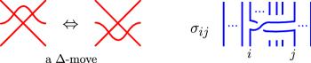
Figure 5: Basics on divide knots

For theory of divide knots, see also [C, HW] and “transverse $\mathbb{C}$-links” defined by Rudolph [R]. In [CP] Couture and Perron pointed out a method to get the braid presentation from the divide in a restricted cases, called “ordered Morse” divides. We can apply their method. It is a special case of Hirasawa’s method in [Hi].

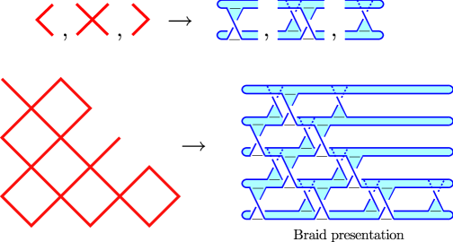
Figure 6: Couture–Perron’s method

Finally we recall an operation “adding a square” on divides $P$ and its contribution to the divide links $L(P)$.

Lemma 2.3 (Lemma 4.2 in [Y4])

Adding a square on an L-shaped curve $P$ along an edge $l$ (of the region) corresponds to a right handed full-twist on the divide knot $L(P)$ along the unknotted component defined by $l$.

Adding a square is related to “blow-down”. Here, blow-down along $y$-axis ($x=0$) is the coordinate transformation from $(x,y)$ to $(x^{\prime},y^{\prime})$ by $x^{\prime}=x,y^{\prime}=yx$ (ex. $y^{2}=x+\epsilon$ become ${y^{\prime}}^{2}={x^{\prime}}^{2}(x^{\prime}+\epsilon)$)

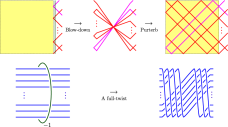
Figure 7: Adding a square

2.3 Curves defined by regions

In $xy$-plane, a lattice point or an integer vector $(k,l)\in\mathbb{Z}^{2}$ is called even or odd, if $k+l$ is even or odd, respectively. Double points of the $\pi/4$-lattice $X=\{(x,y)|\cos\pi x=\cos\pi y\}$ are at even points. In this paper, we are interested in curves constructed as intersection of $X$ and a region, as a generalization of Lemma 2.1.

The lattice $X$ has some symmetries: We let $r_{x}$ denote the reflection along $y$-axis, $r_{x}(x,y)=(-x,y)$, $R_{\pi/2}$ the $\pi/2$-rotation (along the origin), and $+\vec{v}_{\text{ev}}$ a parallel translation by an even vector. Symmetry of the lattice $X$ is generated by $r_{x},R_{\pi/2}$ and some $\vec{v}_{\text{ev}}$. A curve constructed as intersection of $X$ and a region $\mathcal{R}$ does not change by the action (on $\mathcal{R}$) of the symmetry of $X$. We also use a parallel translation $+\vec{v}_{\text{od}}$ by an odd vector to place a region $\mathcal{R}$ well.

Definition 2.4 (Condition of regions)

We are interested in curves constructed as intersection of $X$ and a region $\mathcal{R}$. We formulate the conditions on regions:

1. A region $\mathcal{R}$ is a union of a finite number of rectangles.

2. Each vertex of $\mathcal{R}$ is at a lattice point.

3. Each edge of the rectangles in $\mathcal{R}$ is horizontal or vertical.

4. Difference vectors of any pair of concave points of the region ${\mathcal{R}}$ are even.

Here, a concave point in (iv) is defined as follows: A boundary point $p$ of a region $\mathcal{R}$ is called a concave point (of the region) if a neighborhood of $\mathcal{R}$ at $p$ is locally homeomorphic to that of $\{x\leq 0\}\cup\{y\leq 0\}$ at $(0,0)$ by the symmetry of $xy$-plane, generated by $r_{x}$, $R_{\pi/2}$ and $+\vec{v}$ (by an even or an odd integer vector), see Figure 8.

If a concave point $p$ of $\mathcal{R}$ is at even point, then the curve $X\cap\mathcal{R}$ is not generic at $p$, i.e., a terminal point overlaps with an interior point of the curve. We are concerned only with a generic immersed curves. By the condition (iv), all concave points of either $X\cap\mathcal{R}$ or $X\cap(\mathcal{R}+\vec{v}_{\text{od}})$ are placed at even points, and it defines a generic immersed curve.

Definition 2.5

For a region $\mathcal{R}$ satisfying the condition (i),(ii),(iii) and (iv), either $X\cap\mathcal{R}$ or $X\cap(\mathcal{R}+\vec{v}_{\text{od}})$ is a generic immersed curve. We choose the generic one and define it as a curve defined by the region $\mathcal{R}$, see an example ($X\cap(\mathcal{R}+\vec{v}_{\text{od}})$ is chosen) in Figure 8.

We describe a curve $X\cap\mathcal{R}$ by describing (and parametrizing) the region $\mathcal{R}$ by using $xy$-coordinates.

2.4 Generalized L-shaped curves

We define generalized L-shaped curves. It is an extension of “L-shaped curves” in [Y4, Section 3.2], but the notation (parametrization) is changed.

Definition 2.6 (Generalized L-shaped region at the origin)

See Figure 8.
Let $n$ be a positive integer with $n>1$. We let

$$~{}[(a_{i},b_{i})]:=[(a_{1},b_{1}),(a_{2},b_{2}),\cdots,(a_{n},b_{n})]$$ (2.1)

denote a sequence of lattice points ($\in\mathbb{Z}^{2}$) in $xy$-plane satisfying

$0<a_{1}<a_{2}<\cdots<a_{n}$ and $b_{1}>b_{2}>\cdots>b_{n}>0$.

We define a region $R[(a_{i},b_{i})]$ in $xy$-plane by

$$~{}R[(a_{i},b_{i})]=\bigcup_{i=1}^{n}\{(x,y)|\,0\leq x\leq a_{i},0\leq y\leq b_{i}\}.$$ (2.2)

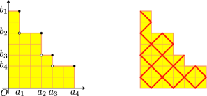
Figure 8: Type $R[(1,7),(3,5),(4,3),(6,2)]$ ($=P(3)$)

We will call this region a generalized L-shaped region of type $[(a_{i},b_{i})]$ of length $n$ (at the origin).

If such a region defines a generic immersed curve in the sense of Definition 2.5, we call the curve generalized L-shaped curve of type $[(a_{i},b_{i})]$.

A generalized L-shaped region of type $[(a_{i},b_{i})]$ of length $n$ has $n-1$ concave points at the coordinate $(a_{i},b_{i+1})$ with $1\leq i\leq n-1$. Note that the L-shaped region $L[a_{1},a_{2};b_{1},b_{2}]$ defined in [Y4, Definition 3.3] is redefined $R[(a_{1},b_{2}),(a_{2},b_{1})]$ of length $2$ here.

It is easy to see:

Lemma 2.7

The area of a generalized L-shaped region of type $[(a_{i},b_{i})]$ of length $n$ is

$$\text{Area }(R[(a_{i},b_{i})])=\sum_{i=1}^{n}a_{i}b_{i}-\sum_{i=1}^{n-1}a_{i}b_{i+1}.$$

Question 2.8

Find a formula on the numbers of circle and arc components of (generic) generalized L-shaped curves. When is a generalized L-shaped curve a generic immersed arc?

2.5 Couture move

We introduce a convenient method Couture move. It was pointed out in the private communication of the author and Olivier Couture in the opportunity of a conference “Singularities, knots, and mapping class groups in memory of Bernard Perron” held in Sept. 2010. The purpose was to present torus knots by generalized L-shaped curves (other than $B(a,b)$ in Lemma 2.1) as divide knots. Here we characterize the move as follows:

Definition 2.9

We say that a deformation of plane curves (divides) is a Couture move if

1. It is from a curve $X\cap\mathcal{R}$ defined by a region $\mathcal{R}$ in the sense of Definition 2.5,

2. The deformation consists of some $\Delta$-moves, and

3. The resulting curve is a curve $X\cap\mathcal{R}^{\prime}$ defined by another region $\mathcal{R}^{\prime}$.

As a demonstration, we prove Lemma 1.5 in the case $j<-1$.

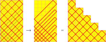
Figure 9: Couture move (ex. $T(6,11)$)

Lemma 2.10

Let $n$ be an integer with $n>1$. We define a sequence $[(a_{i},b_{i})^{(n)}]$ of lattice points of length $n-1$ by

$$(a_{i},b_{i})^{(n)}=(2i,2n+1-2i)\quad(i=1,2,...,n-1).$$

The generalized L-shaped curve of type $[(a_{i},b_{i})^{(n)}]$ presents the torus knot $T(n,2n-1)$ as a divide knot.

Proof. The method is shown in Figure 9, which is an example from $B(5,11)$ to the generalized L-shaped curve of type $[(2,11),(4,9),(6,7),(8,5),(10,3)]$. It consists of some $\Delta$-moves, see Figure 10.

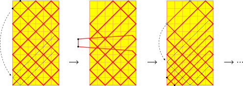
Figure 10: Couture move consists of some $\Delta$-moves

$\Box$

3 Details on sporadic knots and Proof

We give a precise definition of the plane curves $P(j)$, verify the formula in Lemma 1.7 and prove Theorem 1.4 and the lemmas. We start the proof with Baker’s description in [Ba, Ba3] of sporadic knots, and we use Couture moves on divides in the second half of the proof.

3.1 Precise definition of Curves

We define divides $P(j)$ by the method introduced in the last section.

Definition 3.1 (Precise definition of $P(j)$)

For an integer $j$ ($j\not=0,-1$), we define a sequence $[(a_{i},b_{i})^{(j)}]$ of lattice points $(a_{i},b_{i})^{(j)}$ as follows.

(Case $j>0$)  Starting with $[(a_{i},b_{i})^{(1)}]=[(1,3),(2,1)]$, we define $[(a_{i},b_{i})^{(j)}]$ inductively with respective to $j$, by

$$\begin{cases}(a_{1},b_{1})^{(j)}=(1,2j+1)&(i=1)\\ (a_{i},b_{i})^{(j)}=(b_{j+2-i},a_{j+2-i})^{(j-1)}+(1,1)&(1<i\leq j+1)\\ \end{cases}$$

(Case $j<-1$)  We define $[(a_{i},b_{i})^{(j)}]$ by

$$(a_{i},b_{i})^{(j)}=(2i,-2j+1-2i)\quad(1\leq i\leq-j)$$

We define a plane curve $P(j)$ as a generalized L-shaped curve of type $[(a_{i},b_{i})^{(j)}]$, whose length is $j+1$ (if $j>0$) or $-j$ (if $j<-1$). See and verify the examples in Figure 2.

By Lemma 2.7, it is easy to see

Lemma 3.2

$$Area(R[(a_{i},b_{i})^{(j)}])=\begin{cases}2j^{2}+2j&(j>0)\\ 2j^{2}&(j<-1)\\ \end{cases}.$$

The plane curve $P_{\mathcal{X}}(j)$ is constructed by adding a square twice as in Definition 1.3. Since a square addition along an edge $E$ of length $l(E)$ increases the area by $l(E)^{2}$, the area of the region of $P_{IX}(j)$ with $j>0$ is calculated as

$$Area(R[(a_{i},b_{i})^{(j)}])+l(E_{a})^{2}+l(\overline{E_{b}})^{2} = (2j^{2}+2j)+(2j)^{2}+(4j+1)^{2}$$

$$= 22j^{2}+10j+1$$

On the other hand, the area of the region of $P_{X}(j)$ with $j>0$ is calculated as

$$Area(R[(a_{i},b_{i})^{(j)}])+l(E_{b})^{2}+l(\overline{E_{a}})^{2} = (2j^{2}+2j)+(2j+1)^{2}+(4j+1)^{2}$$

$$= 22j^{2}+14j+2$$

We calculate them also in the cases $j<-1$ and list them in Table 2. Lemma 1.7 is proved by Table 2.

Curve	Coeff. $p$ of $k_{\mathcal{X}}(j)$	Area (Case $j>0$)	Area (Case $j<-1$)
$P_{IX}(j)$	$22j^{2}+9j+1$	$22j^{2}+10j+1$	$22j^{2}+8j+1$
$P_{X}(j)$	$22j^{2}+13j+2$	$22j^{2}+14j+2$	$22j^{2}+12j+2$

Table 2: Area of the plane curve $P_{\mathcal{X}}(j)$

Next, we calculate and verify that the numbers of double points of $P(j)$ and $P_{\mathcal{X}}(j)$. By Lemma 2.2(2), they are equal to the genus of the presented knots $L(P(j))$ and $L(P_{\mathcal{X}}(j))=k_{\mathcal{X}}(j)$, respectively. Since $L(P(j))$ is $T(j,2j+1)$ by Lemma 1.5, we have:

Lemma 3.3

The number $d(P(j))$ of double points of the plane curve $P(j)$ is equal to the genus of the torus knot $T(j,2j+1)$:

$$d(P(j))=\frac{(|j|-1)(|2j+1|-1)}{2}=\begin{cases}j(j-1)&(j>0)\\ (j+1)^{2}&(j<-1)\\ \end{cases}.$$

Since the number of double points increases by $l(l-1)/2$ by adding a square along an edge of length $l$, $d(P_{IX}(j))$ is calculated as

(Case $j>0$)

$$d(P_{IX}(j)) = d(P(j))+\frac{l(E_{a})\cdot(l(E_{a})-1)}{2}+\frac{l(\overline{E_{b}})\cdot(l(\overline{E_{b}})-1)}{2}$$

$$= j(j-1)+\frac{2j\cdot(2j-1)}{2}+\frac{(4j+1)\cdot 4j}{2}$$

$$= 11j^{2}$$

(Case $j<-1$)

$$d(P_{IX}(j)) = (j+1)^{2}+\frac{(-2j)\cdot(-2j-1)}{2}+\frac{(-4j-1)\cdot(-4j-2)}{2}$$

$$= 11j^{2}+9j+2$$

They are equal to the genus of the knots $k_{IX}(j)$, see Table 1. We leave the case of TypeX to the readers.

3.2 Proof of the main theorem

In the first half of the proof, we study the knots in the usual diagram and Dehn surgery description. In the second half, we will use divide presentation.

We start with Baker’s Dehn surgery description of the knots $k_{\mathcal{X}}(j)$ in Figure 11 from [Ba]. Throughout the paper, we fix

$$(\alpha,\beta)=\begin{cases}(-2,-3)&\text{ for TypeIX}\\ (-3,-2)&\text{ for TypeX}\end{cases}.$$

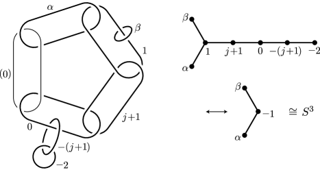
Figure 11: Baker’s description

It is easy to see that the framed sublink of thick seven components presents $S^{3}$, by usual weighted tree diagram in the right half of Figure 11. We call the sublink the non-trivial diagram of $S^{3}$. In the resulting $S^{3}$, the thin component is the sporadic knot $k_{\mathcal{X}}(j)$ as a knot.

[Case $j>0$]  First, we assume that $j>0$ until the final paragraph. To get a usual diagram of the knot $k_{\mathcal{X}}(j)$, we have to chase the thin component (with framing) during the deformation from the non-trivial diagram to the empty diagram of $S^{3}$. It is not easy but straight forward. In the middle of the process, we reach a diagram in Figure 12, where boxed $+1$ in the diagram means a right handed full-twist. The thin component $k(j)$ is a torus knot $T(j,j+1)$ with framing $j(j+1)$, which is a coefficient of reducible Dehn surgery. We name the four component link $L(j)=k(j)\cup u_{-1}\cup u_{\alpha}\cup u_{\beta}$, where $u_{x}$ the $x$-framed unknotted component for $x=-1,\alpha,\beta$.

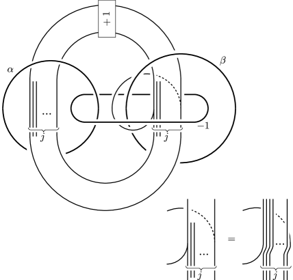
Figure 12: Construction of $k_{\mathcal{X}}(j)$ : Link $L(j)$

Second, we decompose the full-twist at the boxed $+1$ as two half-twists, denoted by $+\frac{1}{2}$ in triangles, and deform the diagram by isotopy as in Figure 13. Note that the half-twist in the right is of $j+1$ strings. We can see that $L(j)$ is strongly invertible with respect to the horizontal axis, see Lemma 2.2(5).

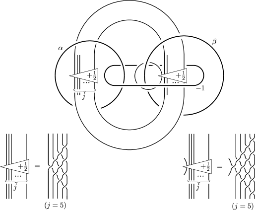
Figure 13: Link $L(j)$ with a strong involution

As a quotient of the involution, ignoring the crossing data (over or under), we have a plane curve properly immersed in the half plane. The curve can be modified as in Figure 14. This is a divide presentation of $L(j)$. It can be checked by Couture–Perron’s method in Figure 6. This process is related to the original construction of divide knots: For a link of singularity of a complex plane curve, the divide is a real part of a “good” perturbation (called real Morsification) of the equation of the singularity.

In the divide presentation of $L(j)$ in Figure 14, a line segment $\ell$ is placed slightly different whether $j$ is even or odd. We name the plane curve $C(j)=c(j)\cup\ell\cup a\cup b$, where $c(j)$ presents $k(j)=T(j,j+1)$ by Lemma 2.1, since $c(j)$ is a generalized L-shaped curve of type $[(j,j+1),(j+1,1)]$ and is isotopic to $B(j,j+1)$. The line segments $\ell,a,b$ presents $u_{-1},u_{\alpha},u_{\beta}$, respectively, as a divide presentation.

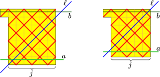
Figure 14: Divide presentation $C(j)$ of $L(j)$  (ex. $j=6$ and $j=5$)

The linking matrix of $L(j)$ with a suitable orientation of the link

$$\begin{pmatrix}j(j+1)&j&j&j+1\\ j&-1&1&1\\ j&1&\alpha&1\\ j+1&1&1&\beta\\ \end{pmatrix},$$

is equal to the matrix of the number of intersection points of the components of the divide by Lemma 2.2(3).

From now on, we go into the second half of the proof, and study the knots and links by divide presentation. We use $\Delta$-moves on divides freely, see Lemma 2.2(7). We have two (or three) steps: (i) Blow-down along $\ell$ (take a full-twist along $u_{-1}$, (ii) (Only if $j$ is odd) Modify the curve by some $\Delta$-moves, and (iii) Deform the curve by Couture moves. Our goal is the divide $P(j)$ with edges $\overline{a},\overline{b}$, where $\overline{a}$ (and $\overline{b}$) is a small parallel push-off of the bottom edge $E_{a}$ (the left edge $E_{b}$) of the region of $P(j)$ into the interior.

(Step (i))  We take a right handed full-twist of $k(j)\cup u_{\alpha}\cup u_{\beta}$ along the unknot $u_{-1}$. We name the resulting link

$$\overline{L(j)}=\overline{k(j)}\cup\overline{u_{\alpha}}\cup\overline{u_{\beta}}.$$

This full-twist is done as a blow-down along the line $\ell$, i.e., by adding a square by Lemma 2.3. In the case where $j$ is even, we slide $\ell$ and $b$ by $\Delta$-moves as the first picture in Figure 15 and add a square. Otherwise, we add a square along the bottom edge as in Figure 16.

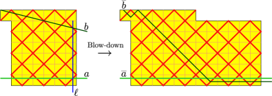
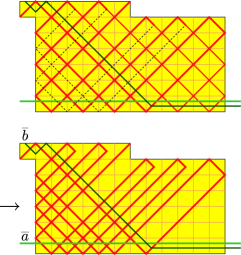
Figure 15: Deformation: Case $j$ is even  (ex. $j=6$)

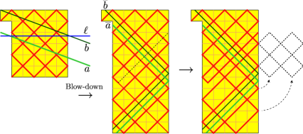
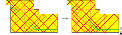
Figure 16: Deformation: Case $j$ is odd  (ex. $j=5$)

(Step (ii)) If $j$ is odd, the curve has a terminal point at the right bottom corner. We move the terminal point (and its segment) up along the right edge, as the second deformation of in Figure 16. We also slide the other added part at the bottom to the right by some $\Delta$-moves.

(Step (iii)) The resulting curve is near L-shaped, but the lines are not in the required position. Here we use Couture move, see the second halves of Figure 15 in the case $j$ is even, and Figure 16 in the case $j$ is odd. By some obvious $\Delta$-moves, we have the required curve $P(j)\cup\overline{a}\cup\overline{b}$, which presents $\overline{L(j)}$ as a divide link.

The sublink $\overline{u_{\alpha}}\cup\overline{u_{\beta}}$ is a Hopf link and the framings are $(\alpha+1,\beta+1)$ $=(-1,-2)$ for TypeIX, or $=(-2,-1)$ for TypeX. By the construction of $P_{\mathcal{X}}(j)$ in Definition 1.3, and by the correspondence between adding a square to a divide and a full-twist of the divide link in Lemma 2.3, we have the required divide presentation of $k_{\mathcal{X}}(j)$ with $j>0$.

[Case $j<-1$]  Finally, we study the case $j<-1$. The method is similar. We define an integer $j^{\prime}$ by $j=-(j^{\prime}+1)$ for figures. Starting with Baker’s description in Figure 11, we have a link $L(j)$ in Figure 17.

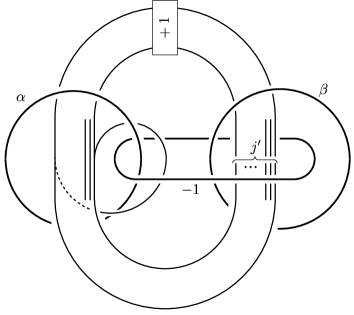
Figure 17: Link $L(j)$ in the case $j<-1$  ($j=-(j^{\prime}+1)$)

Divide description of $L(j)$ is in Figure 18, contrast to Figure 14. Especially, the non-trivial component $c(j)$ and $c(j^{\prime})$ (ex. $c(-6)$ and $c(5)$) are the same curves presenting $T(j,j+1)=T(j^{\prime}+1,j^{\prime})$ but the other segment components are placed differently.

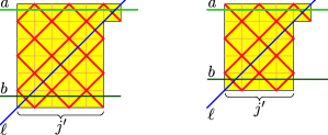
Figure 18: Divide presentation of $L(j)$ with $j<-1$  (ex. $j=-6$ and $j=-5$)

In Figure 19 and 20, we show some deformations. Figures 17, 18, 19, 20 (Case $j<-1$) are contrast to Figures 12, 14, 15, 16 (Case $j>0$), respectively.

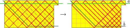
Figure 19: Deformation: Case $j$ is even  (ex. $j=-6$)

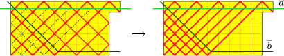
Figure 20: Deformation: Case $j$ is odd  (ex. $j=-5$)

$\Box$

Proof (of Lemma 1.5).  We study a sublink $k(j)\cup u_{-1}$ of $L(j)$ in Figure 12 (or Figure 17, respectively), presented by $c(j)\cup\ell$ in $C(j)$ in Figure 14 (or Figure 18) as a divide link. The component $k(j)$ is a torus knot $T(j,j+1)$ (or $T(j^{\prime}+1,j^{\prime})$). By the diagrams of $L(j)$ in Figure 14 and Figure 18, we can see that $\overline{k(j)}$ is a torus knot $T(j,2j+1)$ (or $T(j^{\prime}+1,2j^{\prime}+1)$), presented by $P(j)$ as a divide knot. The case $j<-1$ is a little harder, see Lemma 2.10. We have the lemma. $\Box$

Proof (of Lemma 1.6).  In [Y3], a divide knot presentation of cable knots (under some conditions) is studied. Here we use $\Delta$-moves on divides freely.

First, assume $j>0$. The plane curve $P_{m}(j)$ is obtained by adding a square twice from $c(j)$ isotopic to $B(j,j+1)$: we add a square along $\ell$ to $c(j)$ first (then we have $P(j)$), and add another square along $E_{a}$ or $\overline{a}$ second. We see the plane curve obtained by the first square addition (blow-down) in Figure 15 or Figure 16. Since the line $\overline{a}$ can be moved to an edge of the L-shaped region by $\Delta$-moves, we can add the second square. The curve becomes an L-shaped curve of type $[(3j,2j),(3j+1,j)]$. By [Y3], it presents the required cable knot $C(T(2,3);j,6j+1)$.

The proof in the case $j<-1$ is similar. From the first curves in Figure 19 or Figure 20, we have an L-shaped curve of type $[(|j|+1,3|j|),(2|j|,3|j|-1)]$. By [Y3], we have the lemma. $\Box$

Acknowledgement. The authors would like to thank to Professor Olivier Couture for his valuable advice in the opportunity of a conference “Singularities, knots, and mapping class groups in memory of Bernard Perron” held in Sept. 2010. Without Couture’s method, the proof would be troublesome and longer. The author would like to thank to Professor Mikami Hirasawa, and Professor Norbert A’Campo for informing him of divide knot theory. The author also would like to thank to Professor Kimihiko Motegi, Professor Toshio Saito, Professor Kenneth L Baker for helpful suggestions on lens space surgery.

This work was supported by JSPS KAKENHI (Grant-in-Aid for Scientific Research) (C) Grant Number 24540070.

YAMADA Yuichi

Dept. of Mathematics, The University of Electro-Communications

1-5-1,Chofugaoka, Chofu, Tokyo, 182-8585, JAPAN

yyyamada=AT=sugaku.e-one.uec.ac.jp

References

- [A1] N A’Campo, Le groupe de monodromie du déploiement des singularité isolées de coubes planes I, Math. Ann. 213 (1975), 1–32.
- [A2] N A’Campo, Generic immersion of curves, knots, monodromy and gordian number, Inst. Hautes Etudes Sci. Publ. Math. 88 (1998), 151–169.
- [A3] N A’Campo, Planar trees, slalom curves and hyperbolic knots, Inst. Hautes Etudes Sci. Publ. Math. 88 (1998), 171–180.
- [A4] N A’Campo, Real deformations and complex topology of plane curve singularities, Ann. de la Faculte des Sciences de Toulouse 8 (1999), 5–23.
- [AGV] V I Arnold, S M Gusein-Zade and A N Varchenko, Singularities of Differentiable Maps, Volume II. Monographs in Mathematics, 83 Birkhauser Boston, Inc., Boston, MA. (1988).
- [Ba] K L Baker, Knots on Once-punctured torus fibers, Ph. D. dissertation, The University of Texas at Austin (2004).
- [Ba2] K L Baker, Surgery descriptions and volumes of Berge knots I: Large volume Berge knots, J. Knot Theory Ramifications 17 (2008), no. 9, 1077–1197.
- [Ba3] K L Baker, Surgery descriptions and volumes of Berge knots II: Description on the minimally twisted five chain link, J. Knot Theory Ramifications 17 (2008), no. 9, 1099–1120.
- [Bg] J Berge, Some knots with surgeries yielding lens spaces, (Unpublished manuscript, 1990).
- [Bg2] J Berge, The knots in which have nontrivial Dehn surgeries that yield , Topology Appl. 38 (1991), no. 1, 1–19.
- [C] S Chmutov, Diagrams of divide links, Proc. Amer. Math. Soc. 131(5) (electronic) (2003), 1623–1627.
- [CP] O Couture and B Perron, Representative braids for links associated to plane immersed curves, J. Knot Theory Ramifications 9 (2000), 1–30.
- [DMM] A Deruelle, K Miyazaki and K Motegi, Networking Seifert surgeries on knots. II. The Berge’s lens surgeries, Topology Appl. 156 (2009), no. 6, 1083–1113.
- [DMM2] A Deruelle, K Miyazaki and K Motegi, Networking Seifert surgeries on knots, Memoirs of the Amer. Math. Soc., 1021 (2012).
- [FS] R Fintushel and R Stern, Constructing Lens spaces by surgery on knots, Math. Z. 175 (1980), 33–51.
- [GHY] H Goda, M Hirasawa and Y Yamada, Lissajous curves as A’Campo divides, torus knots and their fiber surfaces, Tokyo J. Math. 25 (2002), No.2, 485–491.
- [G1] C McA Gordon, Dehn surgery on knots, In Proceedings of the International Congress of Mathematicians (Math. Soc. Japan, 1991), 631–642.
- [G2] C McA Gordon, Dehn filling: a survey, In Knot theory (Banach Center Publ., 1998), 129–144.
- [Hi] M Hirasawa, Visualization of A’Campo’s fibered links and unknotting operations, Topology and its Appl. 121 (2002), 287–304.
- [HW] C V Q Hongler and C Weber, The link of an extrovert divide, Ann. Fac. Sci. Toulouse Math. (6) 9 (2000), no. 1, 133–145
- [OS] R P Osborne and R S Stevens, Group presentations corresponding to spines of -manifolds III, Trans. Amer. Math. 234 (1977), 245–251.
- [R] L Rudolph, Knot theory of complex plane curves, Handbook of Knot Theory, W W. Menasco and M B. Thistlethwaite Eds, Amsterdam: Elsevier. 349-427 (2005).
- [Y1] Y Yamada, Berge’s knots in the fiber surfaces of genus one, lens spaces and framed links, J. Knot Theory Ramifications 14 (2005), no.2, 177–188.
- [Y2] Y Yamada, A family of knots yielding graph manifolds by Dehn surgery, Michigan Math. J. 53(3) (2005), 683–690.
- [Y3] Y Yamada, Finite Dehn surgery along A’Campo’s divide knots, Advanced Studies in Pure Mathematics 43, Singularity Theory and its Applications, (2006), 573-583.
- [Y4] Y Yamada, Lens space surgeries as A’Campo’s divide knots, Algebr. Geom. Topol. 9 (2009), no.1 , 397–428.
- [Y5] Y Yamada, Canonical forms of the knots in the genus one fiber surfaces, Bulletin of the University of Electro-Communications, 22-1 (2010), 25-31.