Blind decomposition of Herschel-HIFI spectral maps of the NGC 7023 nebula

Abstract

Large spatial-spectral surveys are more and more common in astronomy. This calls for the need of new methods to analyze such mega- to giga-pixel data-cubes. In this paper we present a method to decompose such observations into a limited and comprehensive set of components. The original data can then be interpreted in terms of linear combinations of these components. The method uses non-negative matrix factorization (NMF) to extract latent spectral end-members in the data. The number of needed end-members is estimated based on the level of noise in the data. A Monte-Carlo scheme is adopted to estimate the optimal end-members, and their standard deviations. Finally, the maps of linear coefficients are reconstructed using non-negative least squares. We apply this method to a set of hyperspectral data of the NGC 7023 nebula, obtained recently with the HIFI instrument onboard the Herschel space observatory, and provide a first interpretation of the results in terms of 3-dimensional dynamical structure of the region.

Telescopes keep growing in diameter, and detectors are more and more sensitive and made up of an increasing number of pixels. Hence, the number of photons that can be captured by an astronomical instrument, in a given amount of time and at a given wavelength, has raised significantly thus allowing astronomy to go hyperspectral. More and more, astronomers do not deal with 2D images, or 1D spectra, but with a combination of both of these media giving 3D data-cubes (2 spatial dimensions, 1 spectral dimension). The PACS, SPIRE and HIFI instruments, onboard Herschel all have a mode allowing spectral mapping (e.g. van Kempen et al. 2010; Habart et al. 2010; Joblin et al. 2010) in atomic and molecular lines. Owing to its high spectral resolution, HIFI allows to resolve the profiles of these lines, enabling to study the kinematics of e.g. the immediate surrounding of protostars (van Dishoeck et al. 2011), or of star-forming regions (Pilleri et al. 2012) using radiative transfer models.

Although such 3D datasets have become common, there is a lack of methods to analyze the outstanding amount of information they contain. Classical analysis methods tend to decompose the spectra by fitting them with simple functions (typically mixture of gaussians) but this has several disadvantages: 1) the assumption made by the use of a given function usually not based on physical arguments 2) if the number of parameters is high, the result of the fit may be degenerate 3) for large datasets and fitting with nonlinear functions, the fitting may be very time consuming 4) initial guesses must be provided 5) the spectral fitting is usually performed on a (spatial) pixel by pixel basis, so that the extracted components are spatially independent whereas physical components are often present at large scales on the image. Alternatively, it is possible to decompose data-cubes using Principal Component Analysis (e.g. Ungerechts et al. 1997; Brunt & Heyer 2002; Brunt et al. 2009). However this, has the disadvantage to decompose data onto an orthogonal basis, which produces components which are difficult to interpret directly in physical terms (e.g. spectra with negative values). An alternative analysis was proposed by Juvela et al. (1996), which consists in decomposing spectral cubes, in this case spectral maps of the pure rotational lines of carbon monoxide (CO), into the product of a small number of spectral components or “end members” and spatial “abundance” maps, with an enforcement of positivity for all the points in the decomposition. There is no assumption on spectral properties of the components, and hence this can provide deeper insights into the physical structure represented in the data, as demonstrated in this pioneering paper. This method uses the positivity constraint of the maps and spectra (all their points must be positive) combined with the minimization of a statistical criterion to derive the maps and spectral components. This method is referred to as positive matrix factorization (PMF, Paatero 1994). Although it contained the original idea of using positivity as a constraint to estimate a matrix product, this work used a classical optimization algorithm. Several years later, Lee & Seung (1999) introduced a novel algorithm to perform PMF using simple multiplicative iterative rules, making the PMF algorithm extremely fast. This algorithm is usually referred to as Lee and Seung’s Non Negative Matrix Factorization (NMF hereafter) and has been widely used in a vast number of applications outside astronomy. Although some theoretical aspects of this method are still questioned (Donoho & Stodden 2003), this algorithm has proven its efficiency including in astrophysical applications (Berné et al. 2007). However, NMF has several disadvantages: 1) the number of spectra to be extracted must be given by the user and is usually hard to guess 2) the error-bars related to the procedure are not given automatically.

In this paper, we present an alternative way of performing a kinematical study of spectral maps, using a method which combines NMF to a classification algorithm and a Monte-Carlo analysis. This approach tends to discard the standard drawbacks of NMF described above, thus providing a quasi-optimal decomposition. Here we apply this method to Herschel-HIFI spectral maps of the [CII] and ¹³CO(8-7) lines at 1900 and 881 GHz respectively. We describe the algorithms we use in Sect. 1 and the method itself in Sect. 2, and then apply it to the real data.

1 Definitions and algorithms employed by the method

1.1 Mathematical description of the data and aims

In hyperspectral astronomy, the observed data consist of a 3 D $m\times n\times l$ matrix $C(p_{x},p_{y},v)$ where $(p_{x},p_{y})$ define the spatial coordinates and $v$ the spectral index. We assume that all the points in $C(p_{x},p_{y},v)$ are positive. We call spectrum each vector $x(p_{x},p_{y},v)$ recorded at a position $(p_{x},p_{y})$ over the $l$ wavelength points. The goal of the method that we will describe here is to decompose $C$ into the product of a few (typically $<10$) spectra and weight maps using the measured noise in the data as the only input to the method and to provide an error estimation at each point in the extracted spectra. The main algorithms we use here are Lee & Seung’s NMF and K-means which we describe hereafter.

1.2 Lee & Seung’s NMF in our context

We define a new positive 2D matrix of observations $X$, the rows of which contain the $m\times n$, spectra of $C$ arranged in any order. We now assume that each spectrum, $x$, is a linear combination of a limited number $r$ (with $r\ll m\times n$,) of unknown source spectra, i.e.

$$x(p_{x},p_{y},v)=\sum_{i=1}^{r}a^{i}(p_{x},p_{y}){s^{i}(v)}+n(p_{x},p_{y},v),$$ (1)

where $s^{i}(v)$ are source spectra, $i$ is the source index, $a^{i}(p_{x},p_{y})$ are the unknown “weight" coefficients and $n(p_{x},p_{y},v)$ is additive noise. This can be re-written in the following matrix form:

$$X=AS+N,$$ (2)

where $A$ is the $m\times n\times r$ matrix of unknown coefficients of the linear combinations and $S$ is an $r\times l$ matrix, the rows of which are the source spectra and $N$ is the noise matrix. This is a typical blind source separation (BSS) problem (Cardoso 1998), and can be solved using multiple methods (e.g. Lee & Seung 1999, Hyvärinen et al. 2001, Gribonval & Lesage 2006). Here, we use Non-Negative matrix factorization Lee & Seung (1999) that is applicable because $A$ and $S$ are positive. The objective is to find estimates of $A$ and $S$, respectively $W$ and $H$ so that

$$X\approx WH.$$ (3)

This is done by adapting the non-negative matrices $W$ and $H$ so as to minimise the divergence $\delta(X|WH)$, defined as

$$\delta(X|WH) = \sum_{ij}(X^{ij}\log\frac{X^{ij}}{(WH)^{ij}}$$ (5)

$$-X^{ij}+(WH)^{ij}),$$

where the exponents $i$ and $j$ respectively refer to the row and column indexes of the matrices. The algorithm used to achieve the minimization of the divergence is based on the iterative update rule

$$H_{a\mu}\leftarrow H_{a\mu}\frac{\sum_{i}W_{ia}X_{i\mu}/(WH)_{i\mu}}{\sum_{k}W_{ka}},$$

$$W_{ia}\leftarrow W_{ia}\frac{\sum_{\mu}H_{a\mu}X_{i\mu}/(WH)_{i\mu}}{\sum_{\nu}H_{a\nu}}.$$ (6)

Divergence is non increasing under their respective update rules, so that starting from random $W$ and $H$ matrices, the algorithm will converge towards a minimum for $\delta$. This provides the matrix $H$ containing the $r$ estimated source spectra $h_{i}$ (in the following we refer to these as simply “source spectra”). The convergence criterion that we have used here measures the evolution of the divergence as a function of the iteration step. We have assumed that convergence is reached when

$$1-\frac{\delta^{i+1}}{\delta^{i}}<\kappa,$$ (7)

where $\kappa$ is small, typically 0.0001.

1.3 K-means

K-means is a standard unsupervised classification method wich aims to partition a set of vectors into $k$ sets $\sigma=\{\sigma_{1},\sigma_{2},\sigma_{3}\ldots\sigma_{k}\}$ so that within each set, a distance is minimized. In our case, this distance is 1 minus the correlation coefficient. Formally this reads:

$$argmin\sum_{i=1,k}\sum_{h_{j}\in\sigma_{i}}1-corr(h_{j},\mu_{i}),$$ (8)

where $corr$ stands for correlation coefficient and $\mu_{i}$ is the mean spectrum in cluster $\sigma_{i}$. Said in a simple way, K-means as defined here forms clusters that maximize the correlation between vectors within each cluster. The algorithm used to perform K-means is the one provided in Matlab.

2 Architecture of the method

This section describes how we use NMF and K-means as well as a Monte-Carlo (MC) analysis to build our method. The three distinct steps of this method are:

• identification of the number of source spectra based on the difference between the estimated power of noise and reconstruction residuals

• estimation of the source spectra using NMF and errors using MC analysis,

• reconstruction of the weight maps using non-negative least squares.

These steps are described in the following sections.

2.1 Identification of the number of source spectra

The identification of the number of sources in our method relies on the estimation of the norm of the noise matrix $N$ in the data. In real observations $N$ is unknown. However, it is often possible to get an accurate estimation of the power of the noise in the data (this will be described in a subsequent paper, Berné et al. in prep.). Let us consider $\nu_{rms}$, which is an estimation of the Frobenius norm of $N$:

$$\nu_{rms}\sim\|N\|_{F}.$$ (9)

In order to identify the number of source spectra, NMF as described above is applied on $C$ starting with the minimum number of source spectra $r=2$. Once NMF has converged, the matrix of approximated observations $\hat{X}$ is obtained by:

$$\hat{X}=WH.$$ (10)

The norm of residuals (i.e. the difference between original and reconstructed observations) is calculated by:

$$\Psi=\|\hat{X}-X\|_{F}.$$ (11)

If

$$\Psi-\hat{\nu}_{rms}\leq 0,$$ (12)

then the number of sources is $r=2$. If the above inequality is not verified then the algorithm retries for $r=r+1$ and such until Eq. (12) is verified. Note that we do not bring the theoretical proof that $\Psi$ is decreasing when $r$ increases, however, empirical tests on several data-sets (including the one presented in this paper in Sect. 3) show that this is the case.

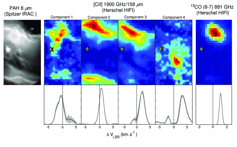
Figure 1: Illustration of the results of our method on the Herschel-HIFI data of the NGC 7023 nebula. On the left, the Spitzer-IRAC images shows the structure of the nebula at mid-infrared wavelengths (polycyclic aromatic hydrocarbon emission). The right part of the figure shows the weight maps (upper panel) and spectral components (lower panel) extracted using the NMF-based method described in this paper. Color-scale and intensities in the spectra are in arbitrary units (due to the scale uncertainty inherent to blind signal separation methods such as NMF). The error intervals ($\epsilon(v)$) as estimated by the method for each source spectrum is shown with the gray envelope (which is very small in the case of the ¹³CO line). The dashed line indicates $\Delta~{}V_{LSR}=0$.

2.2 Monte-Carlo estimation of the source spectra and empirical standard deviation

Once the number of sources $r$ has been identified we can run NMF with this value of $r$ fixed, for $p$ trials, with different initial random matrices for each trial. $p$ is typically 100. For each value trail a set of $r$ source spectra are identified. The total number of obtained spectra at the end of this process is hence $p\times r$. The algorithm uses $K-means$ to form $r$ sets $\{\sigma_{1},\sigma_{2},\ldots\sigma_{r}\}$ each set containing $k_{1},k_{2},\ldots,k_{r}$ spectra. Each final $source$ spectrum is obtained by averaging the $k_{n}$ spectra in each set $\sigma_{n}$. The rows of a new matrix called $H_{*}$ contain these $r$ averaged vectors. The standard deviation at each wavelength $v$ for a given source spectrum is obtained by

$$\epsilon_{n}(v)=\sqrt{\frac{1}{k_{n}-1}\sum_{i=1}^{k_{n}}(h_{i}(v)-\bar{h}(v))^{2}},$$ (13)

where $h_{i}(v)$ is the value of the source spectrum in a set at a given wavelength. $\bar{h}$ denotes the average of $h_{i}(v)$ in the cluster. $\epsilon$ is therefore the empirical sample standard deviation of the value of a point in a $source$ spectrum within its cluster.

2.3 Reconstruction of the weight maps

The matrix of weights $W_{*}$ is reconstructed by minimizing

$$\|X-W_{*}H_{*}\|.$$ (14)

This is done by using the classical non-negative least square algorithm. In the present case we have used the version of this algorithm provided in Matlab.

3 Application to Herschel observations

3.1 Data

The Herschel space telescope is an infrared observatory combining a 3.5 meter telescope and 3 instruments. Here we have used data from the Heterodyne Instrument for Far Infrared (HIFI) which allows spectral mapping at high spectral resolution ($v/\Delta v\sim 10^{6}$) and high angular resolution ($\sim 10-40^{\prime\prime}$) between 480-1250 GHz, and 1410-1910 GHz, as part of the open time program “Physics of gas evaporation at PDR edges” (PI C. Joblin). We have observed the NGC 7023 nebula (Fuente et al. 1996), where a massive star has blown a cavity inside the cloud where it formed. It is illuminated by the young Be star HD200775. With HIFI we have observed the fine structure line emitted by the atomic carbon ion (C⁺) at 1900 GHz as well as the pure rotational line of carbon monoxide isotope ¹³CO(8-7) at 881 GHz in spectral mapping. The resulting data consisting in a 3D matrix of 30$\times$52 spatial positions and 201 spectral points for C⁺ and 18$\times$30 spatial positions and 143 spectral points for the ¹³CO(8-7) spectral map.

3.2 Applying the method to our data

The spectra in this dataset are positive and we assume that non-linear radiative transfer (e.g. re-absorption) effects are not predominant which for the C⁺ and ¹³CO(8-7) line in such physical environment is acceptable. Therefore, the proposed method is applicable. We have applied the method described in Sections 1 and 2 to the dataset presented above. The whole method, implemented under Matlab runs typically in a few minutes when applied to these data. The resulting spectra and weight maps are shown in Fig. 1.

3.3 Preliminary results for C⁺

Four spectra (and weight maps) are identified by the method. Each spatial and spectral component shows distinct features. For clarity, the components can be ordered from 1 to 4 based on their kinematic properties in the following way (Fig. 1):

• Component 1: lowest peak velocity (about -0.8 km s^-1 relative to LSR)

• Component 2: mid peak velocity (about +0.8 km s^-1 relative to LSR)

• Component 3: high peak velocity (about + 2 km s^-1 relative to LSR)

• Component 4: double peaked, very high (+3 km s^-1) and very low (-2 km s^-1) velocity relative to LSR

3.4 Preliminary results for ¹³CO(8-7)

For the ¹³CO(8-7) line we are only able to find two components, one being a complete noise map, so in reality it appears as a unique ¹³CO(8-7) component. This component is shown in Fig. 1.

3.5 Discussion and conclusions

A preliminary interpretation of these results can be formulated. It seems that we are observing the expansion of a roughly symmetric cavity, roughly centered at the peak position in the map of component 4. At this position, we are therefore seeing gas coming towards us and moving away from us at high velocities. The expansion velocity can be derived from this component by taking half of the velocity difference between the two peaks in the spectrum of component 4, that is about 2.5 km s^-1. The other 3 components seem to correspond to the other concentric shells which are expanding at the same velocity, but because of the projection effects their resulting absolute velocities as observed with Herschel are smaller than the expansion velocity of 2.5 km s^-1. The radius of the shell can be estimated using the map of component 2 and taking the distance between the emission peak in the North and the emission peak in the South. This represents an angular size of 60”, that is $R=3.5~{}10^{15}$m in physical scale using a measured distance of 430 parsec. Using this radius and the expansion velocity we can derive the age of the nebula to be $4.5\times 10^{5}$ years. We also note that the center of the expanding shell does not correspond to the position of the star. This is expected since this star is known to have a large proper motion, meaning that it must have moved significantly over the expansion timescale.The exact origin of this expanding shell needs to be investigated in detail, but it is clear that its expansion is driven by the massive star that has formed within the molecular cloud (Fuente et al. 1996). Several scenarios are envisaged: winds and outflow from the star, thermal expansion under irradiation, rocket acceleration of the surrounding cloud due to photo-evaporation etc. Finally, the fact that the CO component, which traces denser regions, appear as a unique component, is compatible with the idea that the warmer gas, traced by the C⁺, is subject to much more dynamical structure because of evaporation. It could also be that there is only one CO component because it traces the edge-on shell which has a higher density than the rest of the expanding shell, that can be seen in C⁺. Further interpretation and modeling is required to take the best advantage of the results obtained here, however, astronomical observations in the far infrared at both high angular and high spectral resolutions, can be interpreted in terms of a linear combination of few components extracted using an NMF based method.

References

- Berné et al. (2007) Berné, O., Joblin, C., Deville, Y., et al. 2007, A&A, 469, 575
- Brunt & Heyer (2002) Brunt, C. M. & Heyer, M. H. 2002, ApJ, 566, 276
- Brunt et al. (2009) Brunt, C. M., Heyer, M. H., & Mac Low, M.-M. 2009, A&A, 504, 883
- Cardoso (1998) Cardoso, J.-F. 1998, Proceedings of the IEEE, 86, 2009
- Donoho & Stodden (2003) Donoho, D. & Stodden, V. 2003, in (MIT Press), 2004
- Fuente et al. (1996) Fuente, A., Martin-Pintado, J., Neri, R., Rogers, C., & Moriarty-Schieven, G. 1996, A&A, 310, 286
- Gribonval & Lesage (2006) Gribonval, R. & Lesage, S. 2006, in ESANN’06 proceedings - 14th European Symposium on Artificial Neural Networks (Bruges, Belgique: d-side publi.), 323–330
- Habart et al. (2010) Habart, E., Dartois, E., Abergel, A., et al. 2010, A&A, 518, L116+
- Hyvärinen et al. (2001) Hyvärinen, A., Karhunen, J., & Oja, E. 2001, Independent component analysis, Vol. 26 (Wiley-interscience)
- Joblin et al. (2010) Joblin, C., Pilleri, P., Montillaud, J., et al. 2010, A&A, 521, L25+
- Juvela et al. (1996) Juvela, M., Lehtinen, K., & Paatero, P. 1996, MNRAS, 280, 616
- Lee & Seung (1999) Lee, D. D. & Seung, H. S. 1999, Nature, 401, 788
- Paatero (1994) Paatero, P. 1994, Environmetrics, 5, 11
- Pilleri et al. (2012) Pilleri, P., Fuente, A., Cernicharo, J., et al. 2012, A&A, 544, A110
- Ungerechts et al. (1997) Ungerechts, H., Bergin, E. A., Goldsmith, P. F., et al. 1997, ApJ, 482, 245
- van Dishoeck et al. (2011) van Dishoeck, E. F., Kristensen, L. E., Benz, A. O., et al. 2011, PASP, 123, 138
- van Kempen et al. (2010) van Kempen, T. A., Kristensen, L. E., Herczeg, G. J., et al. 2010, A&A, 518, L121+