Percolation in the canonical ensemble

Abstract

We study the bond percolation problem under the constraint that the total number of occupied bonds is fixed, so that the canonical ensemble applies. We show via an analytical approach that at criticality, the constraint can induce new finite-size corrections with exponent $y_{\rm can}=2y_{t}-d$ both in energy-like and magnetic quantities, where $y_{t}=1/\nu$ is the thermal renormalization exponent and $d$ is the spatial dimension. Furthermore, we find that while most of universal parameters remain unchanged, some universal amplitudes, like the excess cluster number, can be modified and become non-universal. We confirm these predictions by extensive Monte Carlo simulations of the two-dimensional percolation problem which has $y_{\rm can}=-1/2$.

I Introduction

The bond-percolation model SA can be considered as the $q\rightarrow 1$ limit of the $q$-state Potts model RBP ; FW . Consider a lattice $G\equiv(V,E)$ with $V$ ($E$) the vertex (edge) set, the reduced (divided by $kT$) Hamiltonian of the Potts model reads

$${\mathcal{H}}(K,q)=-K\sum_{ij\in E}\delta_{\sigma_{i}\sigma_{j}}\hskip 28.45274pt(\sigma=1,\cdots,q)\;,$$ (1)

where $K$ is the coupling strength. By introducing bond variables on the edges and integrating out the spin degrees of freedom, one can map the Potts model onto the random-cluster (RC) model. This is the celebrated Kasteleyn-Fortuin transformation KF . The partition sum of the RC model thus assumes the form

$${\mathcal{Z}}_{\rm rc}(u,q)=\sum_{{\mathcal{A}}\subseteq G}\,u^{|{\mathcal{A}}|}q^{k({\mathcal{A}})}\hskip 28.45274pt(u=e^{K}-1)\;,$$ (2)

where the sum is over all the spanning subgraphs ${\mathcal{A}}$ of $G$, $|{\mathcal{A}}|$ is the number of occupied bonds in ${\mathcal{A}}$, and $k({\mathcal{A}})$ is the number of connected components (clusters). The Kasteleyn-Fortuin mapping provides a generalization of the Potts model to non-integer values $q>0$. In the $q\to 1$ limit, the RC model reduces to the bond percolation problem KF ; FW . In this limit, the partition sum assumes the non-singular form $(u+1)^{|E|}$, where $|E|$ is the number of the lattice edges. Nevertheless, rich physics still exists, e.g. in the derivatives of the partition sum involving $q$.

Percolation in two dimensions has been extensively studied. Percolation thresholds on many two-dimensional lattices are exactly known or have been determined to very high precision (see e.g. Ref. Ziff11 and references therein). Most of the critical exponents are also exactly known. For instance, the leading and subleading thermal renormalization exponents are $y_{t}=1/\nu=3/4$ and $y_{i}=-2$, respectively; the leading two critical exponents in the magnetic sector are $y_{h}=d-\beta/\nu=91/48$ and $y_{h2}=71/96$ BNDL ; JCDL . There still exist some critical exponents whose exact values are unknown, including the backbone exponent and the shortest-path fractal dimension GB ; ZYDZ . Much progress has recently been made in the context of the stochastic-Löwner evolution WKBN ; JC .

The present work provides a study of another aspect of percolation. We introduce an “energy-like” constraint that the total number of occupied bonds is fixed and study the effects of such a constraint on the critical finite-size scaling (FSS). Since occupied bonds can formally be considered as particles, we shall refer to percolation under this constraint as percolation in the canonical ensemble, and to the case without the constraint as percolation in the grand-canonical ensemble. Two of us have, for several years, been studying the effects of such constraints DB ; DHB ; DB1 . The leading FSS in systems under energy-like constraints is derived on the basis of the so-called Fisher renormalization MF procedure, which was originally formulated for systems in the thermodynamic limit. Consider an energy-density-like observable $\varepsilon$ in the critical RC model that scales as $\langle\varepsilon(L)\rangle=\varepsilon_{a}+\varepsilon_{s}L^{y_{t}-d}$ in the grand-canonical ensemble, where $L$ is the linear system size and $d$ is the spatial dimensionality. The constraint in the canonical ensemble implies:
(i), $\varepsilon(L)$ for a given size $L$ is fixed at the expectation value $\varepsilon_{a}$ in the thermodynamic limit. This expectation value is normally different from the grand-canonical finite-size average $\langle\varepsilon(L)\rangle$.
(ii), fluctuations of $\varepsilon$ are forbidden—i.e., $\langle\varepsilon^{2}\rangle=\langle\varepsilon\rangle^{2}$.
The effect of (i) is accounted for by the Fisher renormalization. The bond density $|{\mathcal{A}}|/|E|$ is such an observable. For bond percolation, however, since the bond variables on different edges are independent of each other, $\rho_{b}=\langle|{\mathcal{A}}|\rangle/|E|$ does not depend on the system size $L$—i.e., if we write $\rho_{b}=\rho_{b,a}+\rho_{b,s}L^{y_{t}-d}$, then the amplitude $\rho_{b,s}=0$. Thus, percolation provides an ideal system to study the effects of energy-like constraints due to the suppression of fluctuations.

The remainder of this work is organized as follows. Section II describes the sampled quantities and the FSS of physical observables for percolation in the grand-canonical ensemble. Section III derives the effects of the “energy-like” constraint in the critical FSS. The numerical results are presented in Sec. IV. A brief discussion is given in Sec. V.

II Sampled quantities and finite-size scaling

II.1 Simulation and sampled quantities

We consider the bond-percolation problem on an $L\times L$ square lattice with periodic boundary conditions. The grand-canonical simulations follow the standard procedure: each edge is occupied by a bond with probability $p$, after which the percolation clusters are constructed. For simulations in the canonical ensemble, a Kawasaki-like scheme Kawasaki is used. Given an initial configuration with a total number of occupied bonds $|{\mathcal{A}}|=p|E|$, where $|E|=2L^{2}$, an update is defined as the random selection of two edges and the exchange of their occupation states. Each sweep consists of $2L^{2}$ updates. Quantities are sampled after every sweep. Note that although the bond number $|{\mathcal{A}}|=p|E|$ happens to be an integer for the critical square-lattice bond percolation, $p|E|$ is generally a real number. In this case, one can simulate at the ceiling and the floor integer of $p|E|$ and apply an interpolation.

Given a configuration ${\mathcal{A}}$ as it occurs in the simulation, we denote the sizes of clusters as ${\mathcal{C}}_{i}$ ($i=1,\ldots,k({\mathcal{A}})$); ${\mathcal{C}}_{1}$ is reserved for the largest cluster. The following observables were sampled.

1. Energy-like quantities:

   • The bond-occupation density $\rho_{b}=\langle|{\mathcal{A}}|\rangle/|E|$.

   • The cluster-number density $\rho_{k}=\langle k({\mathcal{A}})\rangle/|V|$.

2. Specific-heat-like quantities:

   • $C_{b}=L^{-d}\left(\langle|{\mathcal{A}}|^{2}\rangle-\langle|{\mathcal{A}}|\rangle^{2}\right)$.

   • $C_{k}=L^{-d}\left(\langle k({\mathcal{A}})^{2}\rangle-\langle k({\mathcal{A}})\rangle^{2}\right)$.

   • $C_{kb}=L^{-d}\left(\langle k({\mathcal{A}})\cdot|{\mathcal{A}}|\rangle-\langle k({\mathcal{A}})\rangle\langle|{\mathcal{A}}|\rangle\right)$.

   • $C_{2}=L^{-d}\left(\langle\left[|{\mathcal{A}}|/2+k({\mathcal{A}})\right]^{2}\rangle-\langle|{\mathcal{A}}|/2+k({\mathcal{A}})\rangle^{2}\right)=C_{k}+C_{kb}+C_{b}/4$.

   Here, the factor $1/2$ in the definition of $C_{2}$ arises from the fact that the critical line $u_{c}(q)$ of the RC model (2) on the square lattice is described by $u_{c}(q)=q^{1/2}$, which leads to a weight $q^{|{\mathcal{A}}|/2+k({\mathcal{A}})}$ for a subgraph ${\mathcal{A}}$ along the critical line. In the canonical ensemble, the bond number $|{\mathcal{A}}|$ is fixed, and $C_{b}$ and $C_{kb}$ reduce to $0$.

3. Magnetic quantities:

   • The largest-cluster size $S_{1}=\langle{\mathcal{C}}_{1}\rangle$.

   • The cluster-size moments $S_{\ell}$ ($\ell>1$). Defining ${\mathcal{S}}_{\ell}=\sum_{i}^{k}{\mathcal{C}}_{i}^{\ell}\;,$ we sampled $S_{2}=\langle{\mathcal{S}}_{2}\rangle$ and $\langle 3{\mathcal{S}}_{2}^{2}-2{\mathcal{S}}_{4}\rangle$.

4. Dimensionless quantities:

   • Wrapping probabilities $R_{1},R_{b},R_{x}$, and $R_{e}$. The probability $R_{1}$ counts the events that configuration ${\mathcal{A}}$ connects to itself along the $x$ direction, but not along the $y$ direction; $R_{b}$ is for simultaneous wrapping in both directions; $R_{x}$ is for the $x$ direction, irrespective of the $y$ direction; $R_{e}$ is for wrapping in at least one direction. They are related as $R_{e}=2R_{1}+R_{b}$ and $R_{x}=R_{1}+R_{b}$, thus only two of them are independent NZ ; NZ1 .

   • Universal ratio $Q_{S}=\langle{\mathcal{C}}_{1}^{2}\rangle/S_{1}^{2}$.

   • Universal ratio $Q_{m}=\langle{\mathcal{S}}_{2}\rangle^{2}/\langle 3{\mathcal{S}}_{2}^{2}-2{\mathcal{S}}_{4}\rangle$.

II.2 Finite-size scaling in the grand-canonical ensemble

The critical FSS of the sampled quantities can be obtained from derivatives of the free-energy density $f=-L^{-d}\ln{\mathcal{Z}}_{\rm rc}$ (${\mathcal{Z}}_{\rm rc}$ is given by Eq. (2)) with respect to the thermal scaling field $t$, the magnetic scaling field $h$, or the parameter $q$. In the grand-canonical ensemble, the FSS of $f(q,\,t,\,h,\,L)$ is expected to behave as

$$f(q,\,t,\,h,\,L)=f_{r}(q,\,t,\,h)+L^{-d}f_{s}(q,\,tL^{y_{t}},\,hL^{y_{h}},\,1)\;,$$ (3)

where higher-order scaling fields have been neglected, and $f_{r}$ and $f_{s}$ denote the regular and the singular part of the free-energy density, respectively. The thermal scaling field $t$ is approximately proportional to $u-u_{c}$ in Eq. (2), where $u_{c}(q)=\sqrt{q}$ is the critical line of the $q$-state RC model on the square lattice.

FSS for energy-like quantities. From the partition sum in Eq. (2) and Eq. (3), it can be derived that at criticality

$$(-q)({\rm d}f_{c}/{\rm d}q) = L^{-d}\langle|{\mathcal{A}}|/2+k({\mathcal{A}})\rangle\equiv\rho_{b}(L)+\rho_{k}(L)=\rho_{b,0}+\rho_{k,0}+bL^{-d}\;,$$ (4)

$$(-u/2)(\partial f/\partial u) = 2^{-1}L^{-d}\langle|{\mathcal{A}}|\rangle\equiv\rho_{b}(L)=\rho_{b,0}+aL^{y_{t}-d}\;,$$ (5)

$$(-q)(\partial f/\partial q) = L^{-d}\langle k({\mathcal{A}})\rangle\equiv\rho_{k}(L)=\rho_{k,0}-aL^{y_{t}-d}+bL^{-d}\;,$$ (6)

where $f_{c}=f(u=u_{c})$ is the free-energy density along the critical line $u_{c}(q)=\sqrt{q}$. The last equality in Eq. (4) reflects the analyticity of $f_{c}$ (including the amplitude of its finite-size dependence) along the critical line KZ . Moreover, the correction amplitude $b$ is universal ZFA ; KZ , which is also referred to as the excess cluster number for percolation. The term $\rho_{k,0}$ follows from the exact results for the critical Potts free energy on the square lattice Temperley-71 . An exact result is also available for the triangular lattice BTA . The last equality in Eq. (5) arises from Eq. (3), and $\rho_{b,0}$ accounts for the background contribution; the self-duality of the square-lattice model yields $\rho_{b,0}(q)=1/2$. In the $q\to 1$ limit, the amplitude $a$ vanishes as $a\sim q-1$. Therefore, one has for critical percolation

$$\rho_{b}(L)=\rho_{b,0}\;,\hskip 56.9055pt\rho_{k}(L)=\rho_{k,0}+bL^{-d}\;.$$ (7)

FSS for specific-heat-like quantities. Similarly, one has the second derivatives (at $q=1$) as

$$-\left(q\frac{\rm d}{{\rm d}q}\right)^{2}f_{c} \equiv C_{2}=C_{2,0}+cL^{-d}\;,$$ (8)

$$-\left(u\frac{\partial}{\partial u}\right)^{2}f \equiv C_{b}=C_{b,0}\;,$$ (9)

$$-\left(u\frac{\partial}{\partial u}\right)\left(q\frac{\partial}{\partial q}\right)f \equiv C_{kb}=C_{kb,0}+2a^{\prime}L^{y_{t}-d}+c^{\prime}L^{-d}\;,$$ (10)

$$-\left(q\frac{\partial}{\partial q}\right)^{2}f \equiv C_{k}=C_{k,0}-2a^{\prime}L^{y_{t}-d}+c^{\prime\prime}L^{-d}\;,$$ (11)

where the last equalities in Eq. (10) and (11) arise from the fact that the parameter $a$ in Eqs. (5) and (6) behaves as $a\approx a^{\prime}(q-1)$. The analyticity of $f_{c}$ along the critical line KZ is also reflected in Eq. (8). It is also derived that the amplitude $c$ is a universal quantity KZ , called the excess fluctuation of the number $|{\mathcal{A}}|/2+k({\mathcal{A}})$ for critical bond percolation.

FSS for magnetic quantities. The critical FSS of magnetic quantities can be obtained by differentiating the free-energy density with respect to the magnetic scaling field $h$. It can be shown that at criticality,

$$S_{1}(L)\sim L^{y_{h}}\,,\,\,\,\,S_{2}(L)\sim L^{2y_{h}}\,.$$ (12)

Corrections to FSS. At criticality, the asymptotic behavior of a quantity $O(L)$ is supposed to follow the form

$$O(L)=L^{\psi}(O_{0}+{\rm corrections}),$$ (13)

where $\psi$ is the leading critical exponent and $O_{0}$ is the amplitude. For our observables in bond percolation, values of $\psi$ are given by the previous analysis ($\psi=0$ for dimensionless quantities). The FSS theory predicts several types of “corrections” in Eq. (13) (see e.g. Refs.GOPS and FDB for a review and references therein). These terms include corrections from the irrelevant scaling fields; the leading one has exponent $y_{i}=-2$ for percolation. A regular background term, which appears e.g. as $L^{-y_{h}}$ for $S_{1}$ and $L^{d-2y_{h}}$ for $S_{2}$, contributes to the “corrections”. These regular background terms are also present in the associated dimensionless ratios. For the energy-like quantities ($\rho_{k}$ and $\rho_{b}$) and the specific-heat-like quantities, $\psi$ is negative, thus the regular background (which is $L^{-\psi}$ here) included in the “corrections” in Eq. (13) is actually not a correction, instead it describes the leading behavior, which is the thermodynamic limit of the sampled quantity.

III Finite-size scaling in the canonical ensemble

As mentioned in the Introduction, the critical FSS for bond percolation in the canonical ensemble is due to the suppression of the fluctuation of occupied-bond density $\rho_{b}$. In this section, we demonstrate how the critical FSS is affected by such a suppression.

Without the constraint, any configuration ${\mathcal{A}}$ with bond number $|{\mathcal{A}}|=N_{b}$ occurs with probability $p^{N_{b}}(1-p)^{(N_{e}-N_{b})}$ ($N_{e}=|E|$). Thus, the value $O_{g}$ of an observable $O$ in the grand-canonical ensemble can be written as

$$O_{g}(p,L) = \sum_{N_{b}=0}^{N_{e}}p^{N_{b}}(1-p)^{N_{e}-N_{b}}\sum_{{\mathcal{A}}:|{\mathcal{A}}|=N_{b}}O({\mathcal{A}})\;$$ (14)

$$= \sum_{N_{b}=0}^{N_{e}}p^{N_{b}}(1-p)^{N_{e}-N_{b}}\frac{N_{e}!}{N_{b}!(N_{e}-N_{b})!}O_{c}(\rho,L)\;,$$

where $\rho=N_{b}/N_{e}$ is the occupied-bond density and $O_{c}$ is obtained by averaging over all the configurations ${\mathcal{A}}$ with $|{\mathcal{A}}|=N_{b}$, of which the total number is $N_{e}!/N_{b}!(N_{e}-N_{b})!$. Namely, $O_{c}$ is the canonical-ensemble value of observable $O$. For a sufficiently large system, the binomial distribution in Eq. (14) is well approximated by a Gaussian distribution

$$f(p,\rho,L)=\frac{1}{\sqrt{2\pi}\sigma}e^{-(\rho-{\overline{\rho}})^{2}/{2\sigma^{2}}}\;,\,\,\,\,\sigma=\sqrt{{p(1-p)}/{N_{e}}}\;,$$ (15)

where ${\overline{\rho}}=p$ is the average bond density for occupation probability $p$, and the variance $\sigma$ decreases as $\propto 1/\sqrt{N_{e}}\propto L^{-d/2}$. Thus, Eq. (14) can be re-written as

$$O_{g}(p,L) = \int{\rm d}\rho\;f(p,\rho,L)O_{c}(\rho,L)\;.$$ (16)

In principle, based on the known scaling behavior of $O_{g}$ in the grand-canonical ensemble, the critical FSS of $O_{c}$ can be obtained by the inverse orthogonal transformation of Eq. (16). Here, we take an approximation approach by Taylor expanding $O_{c}(\rho,L)$ in Eq. (16) in powers of $\delta\rho=\rho-{\overline{\rho}}$ about $\rho={\overline{\rho}}=p$, and term-by-term evaluation of the integrals:

$$\int{\rm d}\rho\;f(p,\rho,L)O_{c}(\rho,L) = O_{c}({\overline{\rho}},L)+O_{c}^{\prime}\langle\delta\rho\rangle_{f}+O_{c}^{\prime\prime}\langle(\delta\rho)^{2}/2\rangle_{f}+\ldots$$ (17)

where the derivatives $O_{c}^{\prime}$ and $O_{c}^{\prime\prime}$ are taken at ${\overline{\rho}}$, and the average $\langle\;\;\rangle_{f}$ is over the Gaussian distribution in Eq. (15). It is easily derived that $\langle\delta\rho\rangle_{f}=0$ and $\langle(\delta\rho)^{2}/2\rangle_{f}=p(1-p)/2N_{e}$. Combination of Eqs. (16) and (17) yields

$$O_{g}(p,L)\simeq O_{c}({\overline{\rho}},L)+BO_{c}^{\prime\prime}L^{-d}\;,$$ (18)

with $B=p(1-p)/4$ a non-universal constant.

Near criticality $p_{c}$, we denote $\Delta p=p-p_{c}$. Since ${\overline{\rho}}=p$, we can equivalently denote the distance to the percolation threshold as $\Delta{\overline{\rho}}={\overline{\rho}}-{\overline{\rho}}_{c}$ with ${\overline{\rho}}_{c}=p_{c}$ and $\Delta{\overline{\rho}}=\Delta p$. Thus

$$O_{g}(\Delta p,L) = O_{g,r}(\Delta p)+L^{\psi}[O_{g,s}(L^{y_{t}}\Delta p)+O_{g,i}L^{y_{i}}],$$ (19)

$$O_{c}(\Delta{\overline{\rho}},L) = O_{c,r}(\Delta p)+L^{\psi^{\prime}}[O_{c,s}(L^{y_{\rho}}\Delta p)+B_{\rm can}L^{y_{\rm can}}+O_{c,i}L^{y_{i}}]\;,$$ (20)

where new finite-size corrections with exponent $y_{\rm can}$ are allowed in Eq. (20). It is known from Eq. (20) that $O_{c}^{\prime\prime}({\overline{\rho}}_{c},L)=O_{c,r}^{\prime\prime}+L^{\psi^{\prime}+2y_{\rho}}O_{c,s}^{\prime\prime}$. Taylor-expanding the r.h.s of Eqs. (19-20) and substituting them in Eq. (18) give

$$O_{g,r}(0) + L^{\psi}[O_{g,s}(0)+O_{g,s}^{\prime}L^{y_{t}}\Delta p+O_{g,i}L^{y_{i}}+\ldots]=$$ (21)

$$O_{c,r}(0) + L^{\psi^{\prime}}[O_{c,s}(0)+O_{c,s}^{\prime}L^{y_{\rho}}\Delta p+O_{c,i}L^{y_{i}}+BO_{c,s}^{\prime\prime}L^{2y_{\rho}-d}+B_{\rm can}L^{y_{\rm can}}+BO_{c,r}^{\prime\prime}L^{-d-\psi^{\prime}}+\ldots]$$

Assuming that $2y_{\rho}-d<0$, the term with $O_{c,s}^{\prime\prime}$ acts as a finite-size correction. By comparing the scaling behavior of the l.h.s and the r.h.s. of Eq. (21), we obtain

1. $\psi^{\prime}=\psi$ and $y_{\rho}=y_{t}$,

2. $O_{c,r}(0)=O_{g,r}(0)$, $O_{c,s}(0)=O_{g,s}(0)$ (for $\psi\neq-d$), and $O_{g,s}^{\prime}=O_{c,s}^{\prime}$ etc. In other words, the scaling functions in Eqs. (19) and (20) are identical up to some correction terms.

3. new correction terms appear in the canonical ensemble, and they have exponents $2y_{t}-d$ and $-d-\psi$ (if $-d-\psi<0$). This is because the leading finite-size correction in the l.h.s of Eq. (21) is described by an exponent $y_{i}=-2$, and thus the terms with $L^{2y_{\rho}-d}=L^{2y_{t}-d}$ and $L^{-d-\psi^{\prime}}=L^{-d-\psi}$ have to be cancelled by the newly included correction terms with $L^{y_{\rm can}}$. It can be shown that corrections with exponent $n(2y_{t}-d)$ with $n=2,3,\ldots$ can also occur if higher-order terms are kept in the above Taylor expansions.

4. for the case of $\psi=-d$, $O_{c,s}(0)=O_{g,s}(0)$ does not hold. Instead, one has $O_{g,s}(0)=O_{c,s}(0)+BO_{c,r}^{\prime\prime}$. This predicts that the excess cluster number $b$ in Eq. (7) is changed by the constraint; further, since $B$ and $\rho^{\prime\prime}_{c,r}$ are non-universal, the canonical-ensemble value of $b$ is no longer universal.

Note that the assumption $2y_{\rho}-d<0$ holds since $2y_{t}-d<0$ for percolation in two and higher dimensions.

Finally, we mention that although the constraint is “energy-like”, the derivation applies to both the energy-like and the magnetic observables.

IV Numerical results

To examine the above theoretical derivations, we carry out Monte Carlo simulations for the critical bond percolation on the square lattice, with a fixed bond number $N_{b}=p_{c}|E|=L^{2}$, and for $21$ sizes in range $4\leq L\leq 4000$. The number of samples was about $10^{8}$ for $L\leq 480$, $5\times 10^{7}$ for $L=800$, $2.5\times 10^{7}$ for $L=1600$, and $10^{6}$ for $L=4000$. For the purpose of comparison, additional simulations were also carried out in the grand-canonical ensemble.

IV.1 Evidence for the correction exponent $y_{\rm can}=2y_{t}-d$

We first examine the critical FSS of the wrapping probabilities. In the grand-canonical ensemble, the finite-size corrections arise only from the irrelevant scaling fields for which the leading exponent $y_{i}=-2$. This is illustrated in the inset of Fig. 1. In the canonical ensemble, the existence of the newly induced correction exponent $y_{\rm can}=2y_{t}-d=-1/2$ is clearly demonstrated by the approximately linear behavior for large $L$ in Fig. 1, where $R_{1}$ is plotted versus $L^{-1/2}$.

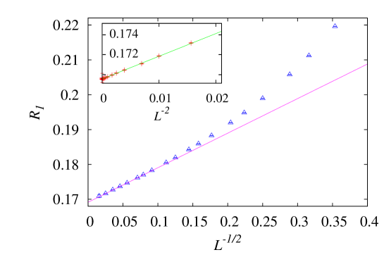
Figure 1: (Color online). Plot of the wrapping probability $R_{1}$ versus $L^{-1/2}$ in the canonical ensemble (main plot). The inset shows $R_{1}$ versus $L^{-2}$ in the grand-canonical ensemble. The straight lines represent the leading finite-size dependence as obtained from the fit. The error bars of the data are smaller than the size of the data points.

According to the least-squares criterion, we fitted the data for these wrapping probabilities by

$$O=O_{0}+B_{1}L^{y_{\rm can}}+B_{2}L^{2y_{\rm can}}+B_{i}L^{y_{i}},$$ (22)

where $O_{0}$ represents the universal value for $L\rightarrow\infty$, and the correction exponent $y_{i}$ is fixed at $-2$. As a precaution against higher-order correction terms not included in the fit formula, the data points for small $L<L_{\rm min}$ were gradually excluded to see how the residual $\chi^{2}$ changes with respect to $L_{\rm min}$. In general, we use results of the fit corresponding to a $L_{\min}$ for which the quality of fit is reasonable, and for which subsequent increases of $L_{\rm min}$ do not cause the $\chi^{2}$ value to drop by vastly more than one unit per degree of freedom. In practice, the word “reasonable” means here that $\chi^{2}$ is less than or close to the number of degrees of freedom, and that the fitted parameters become stable.

Table 1: Fit results for wrapping probabilities. The exact values of $O_{0}$ Pinson ; ZLK , and $y_{i}=-2$ are used here. The abbreviations “GE” and “CE” stand for grand- and canonical ensemble, respectively. Entries “-” indicate the absence of a result, and the numbers without error bars are fixed in the fits. Error margins are quoted as two times of the statistical errors in the fits.

Fit using $O=O_{0}+B_{1}L^{y_{\rm can}}+B_{2}L^{2y_{\rm can}}+B_{i}L^{y_{i}}$
		$O_{0}$	$B_{1}$	$y_{\rm can}$	$B_{2}$	$B_{i}$	$y_{i}$	$L_{\rm min}$
	GE	$0.169\,415\,435$	$-$	$-$	$-$	$0.23(1)$	$-2$	$16$
		$0.169\,415\,435$	$-$	$-$	$-$	$0.24(3)$	$-2.02(4)$	$8$
$R_{1}$		$0.169\,5(4)$	$0.11(2)$	$-0.53(5)$	$-$	$-$	$-$	$160$
	CE	$0.169\,415\,435$	$0.091\,(8)$	$-0.502\,(13)$	$0.08(2)$	$0.56(7)$	$-2$	$12$
		$0.169\,415\,435$	$0.089\,2(5)$	$-1/2$	$0.082\,(4)$	$0.55(3)$	$-2$	$12$
	GE	$0.351\,642\,855$	$-$	$-$	$-$	$-0.254\,(11)$	$-2$	$12$
		$0.351\,642\,855$	$-$	$-$	$-$	$-0.30(5)$	$-2.06(8)$	$8$
$R_{b}$		$0.351\,5(6)$	$-0.10(3)$	$-0.55(7)$	$-$	$-$	$-$	$120$
	CE	$0.351\,642\,855$	$-0.075\,(11)$	$-0.50(2)$	$-0.07(2)$	$-0.53(5)$	$-2$	$8$
		$0.351\,642\,855$	$-0.075\,8(8)$	$-1/2$	$-0.066\,(5)$	$-0.53(3)$	$-2$	$8$
	GE	$0.521\,058\,290$	$-$	$-$	$-$	$-0.021\,(16)$	$-2$	$16$
		$0.521\,058\,290$	$-$	$-$	$-$	$-0.1(1)$	$-2.4(6)$	$8$
$R_{x}$		$0.521\,1(2)$	$0.020\,(4)$	$-0.56(8)$	$-$	$-$	$-$	$32$
		$0.521\,058\,290$	$0.018\,(7)$	$-0.54(8)$	$-$	$-$	$-$	$120$
	CE	$0.521\,058\,290$	$0.014\,(9)$	$-0.51(9)$	$0.016(13)$	$-$	$-$	$16$
		$0.521\,058\,290$	$0.016\,(12)$	$-0.52(11)$	$0.01(3)$	$0.03(8)$	$-2$	$10$
		$0.521\,058\,290$	$0.013\,4(8)$	$-1/2$	$0.016\,(6)$	$0.02(4)$	$-2$	$10$
	GE	$0.690\,473\,725$	$-$	$-$	$-$	$0.22(2)$	$-2$	$16$
		$0.690\,473\,725$	$-$	$-$	$-$	$0.18\,(4)$	$-2.0(1)$	$8$
$R_{e}$		$0.690\,5(6)$	$0.13(3)$	$-0.53(6)$	$-$	$-$	$-$	$120$
		$0.690\,473\,725$	$0.13(3)$	$-0.53(3)$	$-$	$0(7)$	$-2$	$120$
	CE	$0.690\,473\,725$	$0.10(3)$	$-0.50(3)$	$0.13(4)$	$-$	$-$	$40$
		$0.690\,473\,725$	$0.12(3)$	$-0.52(3)$	$0.05(9)$	$0.9(5)$	$-2$	$20$
		$0.690\,473\,725$	$0.102(2)$	$-1/2$	$0.10(2)$	$0.5(3)$	$-2$	$24$

The results are shown in Table 1. The error margins are quoted as two times of the statistical errors in the fits, which also applies to other tables, in order to account for possible systematic errors. The universal values $O_{0}$ can be exactly obtained Pinson ; ZLK . In the grand-canonical ensemble, these exact values of $O_{0}$ were used and the amplitudes $B_{1}$ and $B_{2}$ were set at $0$, so that the fit formula in Eq. (22) has only a single free parameter. Indeed, such a simple formula can well describe the data with $L\geq 16$ for all the wrapping probabilities ($R_{1}$, $R_{b}$, $R_{x}$, and $R_{e}$); further, for $R_{x}$ the amplitude of $B_{i}$ is very small. As expected, including terms with $B_{1}$ and/or $B_{2}$ only yields messy information and does not improve the quality of the fits. In the canonical ensemble, we also fitted the data by Eq. (22) with a single correction term $B_{1}L^{y_{\rm can}}$ ($B_{2}=B_{i}=0$). As shown in Tab. 1, the data up to sufficiently large $L_{\rm min}$ (except $R_{x}$) have to be discarded for a reasonable residual $\chi^{2}$. Nevertheless, we find that (i), the correction term has an exponent close to $-1/2$, and (ii), the estimates of $O_{0}$ agree well with the exact values. A better description of the $R$ data can be obtained by including correction terms with $B_{i}$ and/or $B_{2}$; for simplicity the exact values of $O_{0}$ are used. As a result, the estimates of $y_{\rm can}$ become more accurate, and are in good agreement with the prediction $y_{\rm can}=-1/2$. We note that the correction coefficient $B_{i}$ takes different values in the grand-canonical and the canonical ensemble. This is also in agreement with the theoretical expectation. As predicted in Sec. III, in addition to those with exponent $n(2y_{t}-d)$ $(n=1,2,\ldots)$, correction terms with exponent $-d-\psi$ can also exist in the canonical ensemble. For the wrapping probabilities, one has $\psi=0$ and thus such a correction term has the same exponent as $B_{i}L^{y_{i}}$. Finally, in order to illustrate the term with $L^{2y_{\rm can}}(=L^{-1})$, we plot $\Delta R_{x}=R_{x}-O_{0}-B_{1}L^{y_{\rm can}}$ versus $L^{2y_{\rm can}}$ as in Fig. 2.

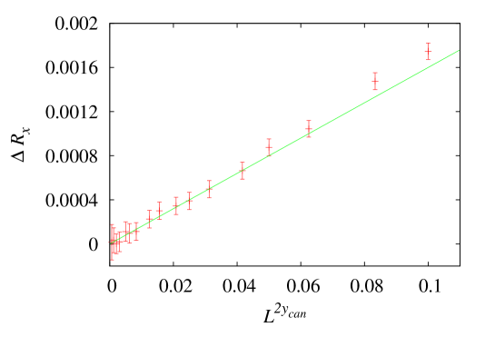
Figure 2: (Color online). Plot of $\Delta R_{x}=R_{x}-O_{0}-B_{1}L^{y_{\rm can}}$ versus $L^{2y_{\rm can}}$ for the canonical wrapping probability $R_{x}$. The straight line represents the leading finite-size dependence of $\Delta R_{x}$, i.e. $B_{2}L^{2y_{\rm can}}$. Parameter $O_{0}$ and $y_{\rm can}$ are fixed at the exact value and $-1/2$ respectively, and the amplitudes $B_{1}$, $B_{2}$ are obtained from the fit.

In order to demonstrate that the correction exponent for the grand-canonical wrapping probabilities is indeed $y_{i}=-2$, we also fitted the data by Eq. (22) with $y_{i}$ being free, $O_{0}$ being fixed at the exact values and $B_{1}=B_{2}=0$. The fit results are also included in Table 1. The result is $-2.02(4)$, $-2.06(8)$, $-2.4(6)$ and $-2.0(1)$, for $R_{1}$, $R_{b}$, $R_{x}$ and $R_{e}$, respectively. These results are in compatible with the existing numerical result $y_{i}=-2.003\,(5)$ NZ1 for $R_{1}$, and agree well with the exact value $y_{i}=-2$. It is interesting to mention that although correction of form $L^{-2}(1+A\log L)$ ($A$ is a constant) has been observed for other observables in the square-lattice bond percolation FDB , there is no evidence for such a logarithmic factor in the finite-size corrections for the wrapping probabilities.

Table 2: Fit results for $S_{1}$, $S_{2}$, and the universal ratios $Q_{S}$ and $Q_{m}$.

Fit using $O=L^{\psi}(O_{0}+B_{1}L^{y_{\rm can}}+B_{r}L^{y_{r}}+B_{i}L^{y_{i}})$
		$O_{0}$	$B_{1}$	$y_{\rm can}$	$B_{r}$	$B_{i}$	$L_{\rm min}$
$S_{1}$	GE	$0.984\,48(3)$	$-$	$-$	$1.7(13)$	$-2(2)$	$32$
	CE	$0.984\,3(4)$	$0.066\,(14)$	$-0.50(5)$	$6(5)$	$-7(6)$	$24$
$S_{2}$	GE	$1.035\,97(4)$	$-$	$-$	$1.7(7)$	$-3.0(14)$	$32$
	CE	$1.035\,8(5)$	$0.05(3)$	$-0.51(12)$	$5(3)$	$-7(5)$	$24$
$Q_{S}$	GE	$0.960\,17(1)$	$-$	$-$	$1.4(8)$	$-1.8(12)$	$40$
	CE	$0.960\,0(3)$	$0.072\,(8)$	$-0.48(4)$	$-$	$-$	$200$
		$0.960\,03(13)$	$0.075\,(5)$	$-0.49(2)$	$-0.3(16)$	$0(2)$	$24$
$Q_{m}$	GE	$0.870\,56(2)$	$-$	$-$	$-1.1(3)$	$1.92(6)$	$32$
	CE	$0.870\,4(2)$	$0.138\,(7)$	$-0.491\,(13)$	$-1.1(6)$	$1.3(9)$	$16$

For magnetic quantities, we consider the largest-cluster size $S_{1}$ and the second cluster-size moment $S_{2}$, as well as the dimensionless ratios. We fitted the data by

$$O=L^{\psi}(O_{0}+B_{1}L^{y_{\rm can}}+B_{r}L^{y_{r}}+B_{i}L^{y_{i}}),$$ (23)

with $y_{i}=-2$ and $\psi$ being fixed at the exactly known value for the two-dimensional percolation. The term with $L^{y_{r}}$ is the correction from the regular background, with $y_{r}=-y_{h}=-91/48$ for $S_{1}$ and $Q_{S}$, and $y_{r}=d-2y_{h}=-43/24$ for $S_{2}$ and $Q_{m}$. The results are shown in Table 2. Again, we find that (i), the values of $O_{0}$ remain unchanged in the canonical ensemble, irrespective of whether they are universal (for $Q_{S}$ and $Q_{m}$) or non-universal (for $S_{1}$ and $S_{2}$), and (ii), new correction terms with an exponent $y_{\rm can}=-1/2$ are introduced. The estimate $Q_{m,0}=0.870\,56(2)$ in the grand-canonical ensemble agrees with the existing result $0.870\,53(2)$ DB1 .

Table 3: Fit results for the cluster-number density $\rho_{k}$ as determined for the bond (BP) and site (SP) percolation problem. Some fits make use of the exact results $\rho^{\rm bond}_{k,0}=0.098\,076\,211$ Temperley-71 and $b_{g}=0.883\,576\,308$ KZ .

Fit using $\rho_{k}=\rho_{k,0}+L^{-2}(b+B_{1}L^{y_{\rm can}}+B_{i}L^{y_{i}})$
		$\rho_{k,0}$	$b$	$B_{1}$	$y_{\rm can}$	$B_{i}$	$L_{\rm min}$
	GE	$0.098\,076\,22(7)$	$0.883\,6(6)$	$-$	$-$	$0.18(3)$	$6$
BP		$0.098\,076\,211$	$0.883\,576\,308$			$0.178\,(14)$	$6$
		$0.098\,076\,21(4)$	$0.23(2)$	$0.57(5)$	$-0.47(6)$	$0.0(4)$	$8$
	CE	$0.098\,076\,211$	$0.226\,(8)$	$0.564\,(12)$	$-0.47(3)$	$-$	$10$
		$0.098\,076\,211$	$0.233\,(4)$	$0.60(2)$	$-1/2$	$-$	$24$
	GE	$0.027\,598\,03(2)$	$0.883\,5(2)$	$-$	$-$	$-0.17(4)$	$16$
SP		$0.027\,598\,02(2)$	$0.883\,576\,308$	$-$	$-$	$-0.22(3)$	$20$
	CE	$0.027\,598\,00(4)$	$0.41(2)$	$0.64(7)$	$-0.46(7)$	$-$	$24$
		$0.027\,597\,99(4)$	$0.417\,(2)$	$0.687\,(11)$	$-1/2$	$-$	$24$

IV.2 Change of the universal excess cluster number

For energy-like quantities, we consider the cluster-number density $\rho_{k}$, and analyze the data by

$$\rho_{k}=\rho_{k,0}+L^{-2}(b+B_{1}L^{y_{\rm can}}+B_{i}L^{y_{i}}),$$ (24)

with $y_{i}=-2$ being fixed. The background term can be exactly obtained as $\rho^{\rm bond}_{k,0}=(3\sqrt{3}-5)/2$ for the critical square-lattice bond percolation Temperley-71 . In the grand-canonical ensemble, the excess cluster number $b$ is known to be universal and the value has been obtained as $b_{g}=0.883\,576\,308$ KZ , with subscript $g$ for the grand-canonical ensemble.

The fit results are given in Table 3. As in the above subsection, the correction term with $y_{\rm can}=-1/2$ is observed in the canonical ensemble, and the background contribution $\rho_{k,0}$ remains unchanged. However, the excess cluster number is now $b_{c}=0.233(4)$, clearly different from the universal value $b_{g}=0.883\,576\,308$ KZ in the grand-canonical ensemble. This indeed confirms the theoretical prediction for the case of $\psi=-2$ in Sec. III. In other words, one expects that $b_{g}=b_{c}+B\rho^{\prime\prime}_{k,r}$, where $B=p(1-p)/4$ is a constant and $\rho^{\prime\prime}_{k,r}$ is the second derivative $\rho^{\prime\prime}_{k,r}$ of the regular part of $\rho_{k}$ with respect to the bond density. Since both $B$ and $\rho^{\prime\prime}_{k,r}$ are non-universal, the canonical-ensemble value $b_{c}$ is no longer universal. As an illustration, we plot $\rho_{k}$ versus $L^{-2}$ in Fig. 3, where the difference of $b_{g}$ and $b_{c}$ is reflected by the different slopes of the data lines.

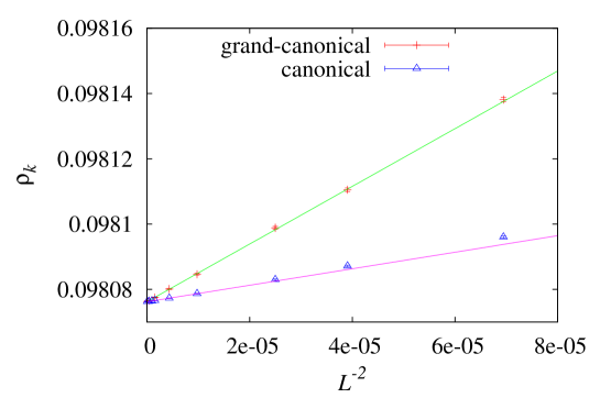
Figure 3: (Color online). Plot of the cluster-number density $\rho_{k}$ versus $L^{-2}$ for the bond percolation model. The straight lines represent the leading finite-size dependence of $\rho_{k}$ as obtained from the fit.

In order to examine the “non-universal” nature of the excess cluster number $b_{c}$ in the canonical ensemble, we also performed simulations of square-lattice site-percolation problem at the percolation threshold $p^{\rm site}_{c}=0.592\,746\,02$ Lee ; FDB ; Ziff11 . In the grand-canonical ensemble, the simulations used 15 system sizes in range $4\leq L\leq 512$, and the results of the fits by Eq. (24) are given in Tab. 3. The estimate of $b_{g}=0.883\,5(2)$ agrees well with the universal value $0.883\,576\,308$ KZ .

In the canonical ensemble, the total number of occupied sites $N_{s}(L)=p^{\rm site}_{c}L^{2}$ is fixed. However, $N_{s}(L)$ is not an integer, and thus the actual simulations were carried out for the total occupied-site number $[N_{s}(L)]$ and $[N_{s}(L)]+1$, with $[\;]$ for the floor integer. The Monte Carlo results at $N_{s}(L)$ were then obtained by linear interpolation. The simulations used $16$ system sizes $L$ in range $4\leq L\leq 1024$. The results of fits using Eq. (24) are also given in Tab. 3. As expected, one has a correction term with exponent $-1/2$ and $b_{c}^{\rm(site)}[=0.417(2)]\neq b_{g}$. The “non-universal” property of $b_{c}$ is demonstrated by the fact $b_{c}^{\rm(site)}\neq b_{c}^{\rm(bond)}$.

In addition, from our fits, one gets $\rho^{\rm site}_{k,0}=0.027\,598\,00(5)$, which is in good agreement with the existing result $0.027\,598\,1(3)$ ZFA , and reduces the error margin significantly.

We also study the FSS of the specific-heat-like quantity $C_{2}$ for the bond percolation model and find that due to the limited precision, the data for $L\geq 8$ are well described by $C_{2}(L)=C_{2,0}+cL^{-2}$. As already mentioned in Section II, the excess fluctuation $c$ is universal. In the grand-canonical ensemble, the fit yields $C_{2,0}=0.039\,446\,(4)$ and $c_{g}=0.105\,5(7)$; the former is consistent with the existing result $C_{2,0}=0.039\,44(4)$ DY , the latter agrees well with the exactly known value $c=0.105\,436\,634$ KZ . In the canonical ensemble, the result is $C_{2,0}=0.039\,446\,(6)$ and $c_{c}=-0.33(5)$. It is interesting to observe that not only the magnitude of the excess fluctuation $c$ is modified, but that also its sign has changed.

IV.3 Universality of scaling functions

In Sec. III, we state that the scaling functions in Eqs. (19) and (20) are identical up to some correction terms, which reflects the universality of the functions. In order to demonstrate this, we carried out simulations near the critical point. We plot the grand-canonical $R_{x}$ versus $L^{y_{t}}(p-p_{c})$ and the canonical $R_{x}$ versus $L^{y_{t}}({\overline{\rho}}-{\overline{\rho}}_{c})$ as in Fig. 4. As expected, data points in both the ensembles nicely collapse to the same curve.

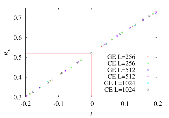
Figure 4: (Color online). Plot of $R_{x}$ versus $t$ for bond percolation. Parameter $t$ represents $L^{y_{t}}(p-p_{c})$ in the grand-canonical ensemble (GE), and $L^{y_{t}}({\overline{\rho}}-{\overline{\rho}}_{c})$ in the canonical ensemble (CE). The excellent collapse demonstrates the universality of scaling functions near the critical point.

V Discussion

We derive the critical finite-size scaling behavior of percolation under the constraint that the total number of occupied bonds/sites is fixed, and confirm theoretical predictions for the two-dimensional percolation by means of Monte Carlo simulation in two dimensions. In particular, it is found that with the constraint, new finite-size corrections with exponent $n(2y_{t}-d)$ $(n=1,2,\ldots)$ are induced and the excess cluster number becomes non-universal. We note that our theory in Sec. III can be used to explain the observed correction exponent $\approx-0.5$ for the canonical wrapping probabilities in simulating the two-dimensional percolation by the Newman-Ziff algorithm NZ ; NZ1 . The predictions should be valid in any dimension with $d\geq 2$. We believe that this work provides an additional useful reference for percolation—a pedagogical system in the field of statistical mechanics. Furthermore, our work can help to understand the critical finite-size-scaling properties of other statistical systems in the canonical ensemble with a fixed total number of particles, which is the usual situation during experiments.

References

• (1) Stauffer D and Aharony A 1994 Introduction to Percolation Theory revised 2nd edn (London: Taylor & Francis)
• (2) Potts R B 1952 Proc. Cambridge Philos. Soc. 48 106
• (3) Wu F Y 1978 J. Stat. Phys 18 115
• (4) Kasteleyn P W and Fortuin C M 1969 J. Phys. Soc. Japan 26 (Suppl.) 11
Fortuin C M and Kasteleyn P W 1972 Physica (Amsterdam) 57 536
• (5) Ziff R M 2011 Phys. Procedia 15 106
• (6) Nienhuis B 1987 Phase Transitions and Critical Phenomena vol 11 ed Domb C and Lebowitz J L (London: Academic) p 1
• (7) Cardy J L 1987 Phase Transitions and Critical Phenomena vol 11 ed Domb C and Lebowitz J L (London: Academic) p 55
• (8) Grassberger P 1992 J. Phys. A 25 5475
Grassberger P 1992 J. Phys. A 25 5867
Grassberger P 1999 Physica A 262 251
• (9) Zhou Z, Yang J, Deng Y and Ziff R M 2012 arXiv:1112.3428 and references therein
• (10) Kager W and Nienhuis B 2004 J. Stat. Phys. 115 1149
• (11) Cardy J L 2005 Ann. Phys. 318 81
• (12) Deng Y and Blöte H W J 2004 Phys. Rev. E 70 046111
• (13) Deng Y, Heringa J R and Blöte H W J 2005 Phys. Rev. E 71 036115
• (14) Deng Y and Blöte H W J 2005 arXiv:cond-mat/0508348
• (15) Fisher M E 1968 Phys. Rev. 176 257
• (16) Kawasaki K 1972 Phase Transitions and Critical Phenomena vol 2 ed Domb C and Green M (London: Academic) p 443
• (17) Newman M E J and Ziff R M 2000 Phys. Rev. Lett. 85 4104
• (18) Newman M E J and Ziff R M 2001 Phys. Rev. E 64 016706
• (19) Kleban P and Ziff R M 1998 Phys. Rev. B 57 R8075
• (20) Ziff R M, Finch S R and Adamchik V S 1997 Phys. Rev. Lett. 79 3447
• (21) Temperley H N V and Lieb E H 1971 Proc. R. Soc. Lond. A. 322 251
• (22) Baxter R J, Temperley H N V and Ashley S E 1978 Proc. R. Soc. Lond. A. 358 535
• (23) Garoni T M, Ossola G, Polin M and Sokal A D 2011 J. Stat. Phys. 144 459
• (24) Feng X, Deng Y and Blöte 2008 Phys. Rev. E 78 031136
• (25) Pinson H T 1994 J. Stat. Phys. 75 1167
• (26) Ziff R M, Lorenz C D and Kleban P 1999 Physica A 266 17-26
• (27) Lee M J 2008 Phys. Rev. E 78 031131
• (28) Deng Y and Yang X 2006 Phys. Rev. E 73 066116