The Ising Spin Glass in dimension five : link overlaps

Abstract

Extensive simulations are made of the link overlap in five dimensional Ising Spin Glasses (ISGs) through and below the ordering transition. Moments of the mean link overlap distributions (the kurtosis and the skewness) show clear critical maxima at the ISG ordering temperature. These criteria can be used as efficient tools to identify a freezing transition quite generally and in any dimension. In the ISG ordered phase the mean link overlap distribution develops a strong two peak structure, with the link overlap spectra of individual samples becoming very heterogeneous. There is no tendency towards a ”trivial” universal single peak distribution in the range of size and temperature covered by the data.

We have studied the spin and link overlaps (defined below, Eqs. 1 and 2) in some detail for cubic Ising Spin Glasses (ISGs) with near neighbor interactions in dimension five. The apparently perverse choice of dimension five, just below the ISG upper critical dimension $d_{\mathrm{ucd}}=6$, has a number of motivations. ISGs in this dimension have almost never been studied through simulations, but there are precise and reliable estimates for the inverse critical temperatures from High Temperature Series Expansion (HTSE) calculations daboul:04 . In terms of numbers of spins $N$ the sizes $L=4,6$ and $8$ used here are equivalent to three dimensional samples of size $L=10,20$ and $32$, so from the point of view of $N$ the present samples are ”large”. However, for the same $N$ equilibration to criticality and beyond is much faster than in lower dimensions.

We first show that at the ordering temperature the moments of the mean link overlap distributions show characteristic peaks, reflecting the onset of correlated spin clusters. This phenomenon can provide both fundamental information on the ordering process and an efficient tool for the accurate evaluation of critical temperatures, in any dimension and for any interaction distribution.

Then in the ordered state, rather than measuring large numbers of samples and averaging over the observables recorded, we take an alternative approach. We study a limited number of samples ($32$ for each size) and record explicitly the equilibrium spin overlap $P(q)$ and link overlap $Q(q_{\ell})$ spectra for each individual sample over a succession of inverse temperatures. Examples of individual $P(q)$ distributions for ISGs have been exhibited in the literature, whereas for the link overlaps only mean $[Q(q_{\ell})(L,\beta)]$ distributions ciria:93 ; katzgraber:01 ; hed:07 ; contucci:07 ; leuzzi:08 ; janus:10 but no individual sample $Q(q_{\ell})$ spectra have been published as far as we are aware. It turns out that individual ISG samples in fact show strongly idiosyncratic link overlap spectra which provide insight into the controversial question of the structure of the SG ordered phase.

The link overlap parameter caracciolo:90 in ISG numerical simulations is the bond analogue of the intensively studied spin overlap. In both cases two replicas (copies) $A$ and $B$ of the same physical system are first generated and equilibrated; updating is then continued and the ”overlaps” between the two replicas are recorded over long time intervals. The spin overlap at any instant $t$ corresponds to the fraction $q(t)$ of spins in $A$ and $B$ having the same orientation (both up or both down), and the normalized overall distribution over time is written $P(q)$. The link overlap corresponds to the fraction $q_{\ell}(t)$ of links (or bonds or edges) between spins which are either both satisfied or both dissatisfied in the two replicas; the normalized overall distribution over time is written $Q(q_{\ell})$. The explicit definitions are

$$q(t)=\frac{1}{N}\,\sum_{i=1}^{N}S_{i}^{A}(t)S_{i}^{B}(t)$$ (1)

and

$$q_{\ell}(t)=\frac{1}{N_{\ell}}\sum_{ij}S_{i}^{A}(t)S_{j}^{A}(t)S_{i}^{B}(t)S_{j}^{B}(t)$$ (2)

where $N$ is the number of spins per sample and $N_{l}$ the number of links; spins $i$ and $j$ are linked, denoted by $ij$. We will indicate means taken over time for a given sample by $\langle\cdots\rangle$ and means over sets of samples by $[\cdots]$. The physical distinction between the information obtained from $P(q)$ and $Q(q_{\ell})$ is frequently illustrated in terms of a low temperature domain picture bokil:00 .

The Hamiltonian is as usual

$$\mathcal{H}=-\sum_{ij}J_{ij}S_{i}S_{j}$$ (3)

with the interactions the symmetric bimodal ($\pm J$) or Gaussian distributions normalized to $\langle J_{ij}^{2}\rangle=1$. We will quote inverse temperatures $\beta=1/T$. $\beta_{c}=0.3925(35)$ for the bimodal case and $\beta_{c}=0.420(3)$ for the Gaussian from HTSE calculations daboul:04 . Equilibration and measurement runs were performed by standard heat bath updating (without parallel tempering) on randomly selected sites. Each sample started at infinite temperature and was gradually cooled until it reached its final temperature. For temperatures near $T_{c}$ each sample saw at least $10^{7}$ sweeps before reaching its final temperature. Then another $10^{7}$ sweeps were run before any measurements took place. Normally there were about 10 sweeps between measurements, though less for higher temperatures and more for lower temperatures. At each temperature and sample we collected $4\cdot 10^{5}$, $6\cdot 10^{5}$ and $5\cdot 10^{6}$ measurements for $L=8$, $6$ and $4$ respectively.

For the Gaussian ISG it has been shown katzgraber:01 that in equilibrium

$$[\langle q_{\ell}\rangle(L,\beta)]=1-[\langle|U|\rangle(L,\beta)]/\beta$$ (4)

where $[\langle|U|\rangle(L,\beta)]$ is the mean energy per bond. The Gaussian data presented here satisfy this equilibrium condition over the full temperature range used; the bimodal samples equilibrated faster than the Gaussian ones and were equilibrated for as long times so we will consider that for present purposes effective equilibration has been reached. However we will note elsewhere that the condition Eq. (4) is necessary but not stringent enough for true equilibration.

For the symmetric bimodal ISG there are simple rules on $\langle q_{\ell}\rangle$. If $p_{s}(\beta)$ is the probability that a bond is satisfied,

$$|U(\beta)|\equiv 1-2p_{s}(\beta)$$ (5)

and a strict lower limit on $\langle q_{\ell}\rangle$ (uncorrelated satisfied bond positions) is given by

$$[\langle q_{\ell}\rangle(L,\beta)]\geq p_{s}^{2}+(1-p_{s})^{2}-2p_{s}(1-p_{s})\equiv[U(L,\beta)^{2}].$$ (6)

In the high temperature limit $|U|(\beta)\to\tanh(\beta)$ so

$$[\langle q_{\ell}\rangle(L,\beta)]/[(1-|U(L,\beta)|/\beta)]\to 3.$$ (7)

For a pure near neighbor ferromagnet (so with translational invariance) $[\langle q_{\ell}\rangle(L,\beta)]\equiv[U(L,\beta)^{2}]$ at all temperatures.

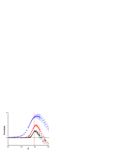
Figure 1: (Color online) The mean Q-kurtosis Eqn. (8) for the sets of bimodal samples with $L=4$ (blue triangles), $L=6$ (red circles) and $L=8$ (black squares).

In addition to the mean $[\langle q_{\ell}\rangle(\beta)]$, important complementary information can be obtained from the moments of the $Q(q_{\ell})$ distributions. The mean Q-kurtosis can be defined by

$$Q_{k}=\left[\left\langle\left(q_{\ell}-\langle q_{\ell}\rangle\right)^{4}\right\rangle\Big{/}\left\langle\left(q_{\ell}-\langle q_{\ell}\rangle\right)^{2}\right\rangle^{2}\right]$$ (8)

and the mean Q-skewness by

$$Q_{s}=\left[\left\langle\left(q_{\ell}-\langle q_{\ell}\rangle\right)^{3}\right\rangle\Big{/}\left\langle\left(q_{\ell}-\langle q_{\ell}\rangle\right)^{2}\right\rangle^{3/2}\right]$$ (9)

For the bimodal ISG the distributions are Gaussian at high temperatures ($Q_{k}=3,Q_{s}=0$), with peaks in the mean $Q_{k}(L,\beta)$ and $Q_{s}(L,\beta)$ at criticality, Figure 1. The amplitudes of the peaks decrease with increasing $L$; this could be called an ”evanescent” critical phenomenon as it will disappear in the thermodynamic limit. Allowing for a weak finite size correction term, the positions of the maxima $\beta_{max}$ for each set of peaks tend accurately towards the HTSE $\beta_{c}$ with increasing $L$. For the Gaussian ISG an analogous peak behavior is observed.

Physically, the excess Q-kurtosis (”fat tailed” distributions) and Q-skewness near $\beta_{c}$ in ISGs must be related to the build up of inhomogeneous temporary correlated spin clusters around criticality. The data show that they appear when the thermodynamic limit correlation length ratio $\xi(\beta)/L$ is greater than some value; then the Q-kurtosis and the Q-skewness each tend to a peak for fixed $L$ as $\xi(\beta)$ diverges, so at $\beta_{c}$. This simple argument explains why in ISGs the peaks should be situated exactly at $\beta_{c}$ in the large $L$ limit. Indeed we will show elsewhere that excess Q-kurtosis and Q-skewness peaks are not unique to ISGs; analogous behavior with peaks tending to precisely $\beta_{c}$ with increasing size is observed in a pure Ising ferromagnet, where the data are not subject to sample averaging noise lundow:12a . Potentially Q-kurtosis and Q-skewness measurements could be used as a standard procedure for estimating critical temperatures. This method would not have the intrinsic disadvantages of the usual crossing point techniques.

Turning to the ordered phase $\beta>\beta_{c}$, a longstanding controversy concerns the correct physical description of ISGs for finite dimensions parisi:83 ; fisher:86 . Generally the arguments are focussed on the behavior to be expected at very large sizes and very low temperatures. Unfortunately in practice the combination of these limits renders direct observations inaccessible to numerical simulations, so the conclusions must rely on extrapolations. Here our aim is to reach a phenomenological description of an ensemble of individual samples of limited size at temperatures somewhat below the critical temperature, so in a region which can be studied directly by simulations.

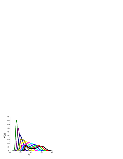
Figure 2: (Color online) The mean $L=6$ link overlap distributions $[Q(q_{\ell})(L,\beta)]$ for inverse temperatures $\beta=0.40,0.42,0.44,0.46,0.48,0.50,0.52,0.54,0.56,0.58,0.60$ (from left to right; olive,purple,navy, brown, yellow, pink, cyan, blue, green, red, black).

In Figure 2 we show mean bimodal link overlap spectra $[Q(q_{\ell})]$ averaged over the $32$ sample set at $L=6$ and $\beta$ up to $0.60$. Broadly similar double peak spectra have been observed in other ISG measurements in dimensions $3$ and $4$ ciria:93 ; katzgraber:01 ; hed:07 but the present mean spectra resemble even more closely mean field regime spectra in dimension $1$ with algebraically decaying interactions (Leuzzi et al Figure 2 leuzzi:08 ). The presence of secondary peaks in mean $[Q(q_{\ell})]$ spectra was explained by Bokil et al bokil:00 as being due to the coexistence of a monodomain configuration and a domain wall configuration, with the secondary peak corresponding to one of the two replicas residing in one of these configuration and the other replica in the other. By analogy with results they had obtained on a Migdal-Kadanoff model, Bokil et al predicted that the secondary peak would melt rapidly into the main peak with increasing $L$. This is not what we observe. As in the mean field case the secondary peak becomes more and more cleanly separated as the size is increased and as the temperature is lowered. There appears to be no tendency towards ”trivial” single peak $[Q(q_{\ell})]$ structure in the range of $L$ and $\beta$ covered by the present data.

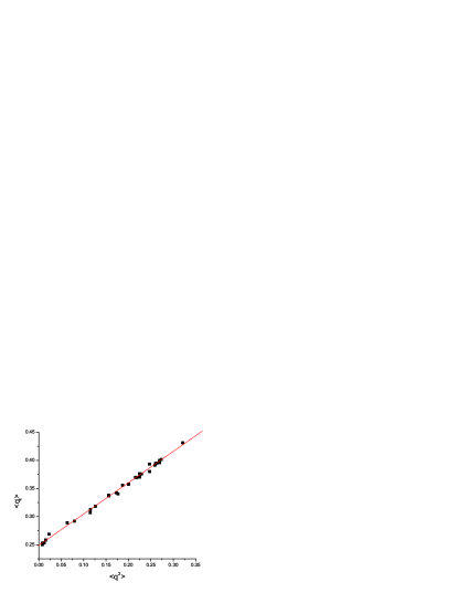
Figure 3: (Color online) A scatter plot of the link overlap $\langle q_{\ell}\rangle$ against the square of the spin overlap $\langle q^{2}\rangle$ for the set of $32$ bimodal samples with $L=6$ at $\beta=0.60$.

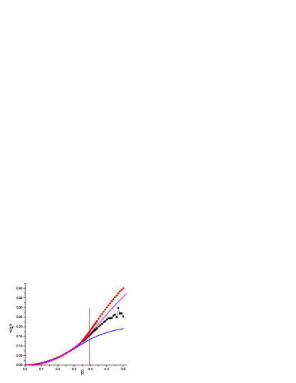
Figure 4: (Color online) The temperature dependence of the link overlap $\langle q_{\ell}\rangle(\beta)$ for two extreme $L=6$ bimodal samples : sample $\#22$ (red circles) and sample $\#02$ (black squares) together with the mean $[\langle q_{\ell}\rangle(\beta)]$ for the $L=6$ set (upper pink curve) and the square of the energy per link $[U(\beta)^{2}]$ (lower blue curve). The vertical line indicates the HTSE critical $\beta{c}=0.3925$.

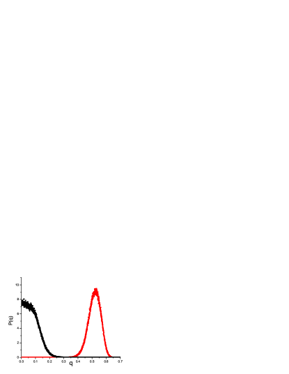
Figure 5: (Color online) The spin overlap distribution spectra $P(q)(\beta)$ for the $L=6$ samples $\#22$ (red, right hand curve)and $\#02$ (black, left hand curve) at $\beta=0.60$. (The spectra are symmetric about $q=0$).

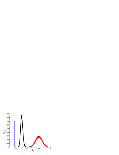
Figure 6: (Color online) The link overlap distribution spectra $Q(q_{\ell})(\beta)$ for the $L=6$ samples $\#22$ (red, right hand curve) and $\#02$ (black, left hand curve) at $\beta=0.60$. The vertical blue line is the strict random link limit $\langle q_{\ell}(\beta)\rangle=[U(\beta)^{2}]$.

It is of interest to go into more detail and to examine the behavior of the distributions $P(q)$ and $Q(q_{\ell})$ for individual samples (see for instance yucesoy:12 for $P(q)$). Each of the $32$ realization sets can be taken as an unbiased sampling of the entire population of possible realizations for a given size and temperature. Only a couple of these spectra can be exhibited here. In Figure 3 we show a scatter pattern of $\langle q_{\ell}\rangle$ against $\langle q^{2}\rangle$ for the $32$ sample set of $L=6$ individual bimodal samples at the lowest temperature studied $\beta=0.60\sim 1.5\beta_{c}$. It can be seen that $\langle q^{2}\rangle$ and $\langle q_{\ell}\rangle$ are correlated linearly as would be expected on the grounds of overlap equivalence contucci:06 . We select two extreme samples from this set, $\#22$ with the highest and $\#02$ with the lowest average $\langle q_{\ell}\rangle$. The temperature dependence of $\langle q_{\ell}\rangle(\beta)$ for these samples together with the mean $[\langle q_{\ell}\rangle(\beta)]$ and $[U(\beta)^{2}]$ are shown in Figure 4. The degree of localization of the satisfied links can be considered to be represented by the difference between $\langle q_{\ell}\rangle(\beta)$ and the random link position limit $[U(\beta)^{2}]$. It can be seen that both samples begin to localize their links somewhat before $\beta_{c}$; when the temperature is lowered further, the localization in sample $\#22$ is always about twice as strong as that of sample $\#02$. When the same procedure is followed for $L=4$ and $L=8$ or for the Gaussian interaction samples, very similar results are obtained.

Finally we show, Figures 5 and 6, individual $P(q)$ and $Q(q_{\ell})$ spectra for these extreme samples at $\beta=0.60$. Both on the Replica Symmetry Breaking (RSB) parisi:83 and the droplet fisher:86 approaches one expects for individual spectra principal Edwards-Anderson (EA) self-overlap peaks at $q=\pm q(EA)$) and $q_{\ell}=q_{\ell}(EA)$, together with [RSB] or without [droplet] secondary peaks. The high extreme sample $\#22$ spectra follow the simple droplet pattern and are ”trivial”, but remarkably for the low extreme sample $\#02$, where the $P(q)$ spectrum is concentrated around $q=0$, the $Q(q_{\ell})$ spectrum shows essentially no weight at an EA peak position anywhere near that of the other spectrum. The entire $Q(q_{\ell})$ spectrum for this sample (and others like it) is concentrated around the mean spectrum secondary peak position in Figure 2, so in the sense of Bokil et al it is ”all wall”. It is samples of this type which are contributing the most strongly to the secondary peak in the mean $[Q(q_{\ell})]$ spectra. The only plausible interpretation which suggests itself for these spectra lacking EA self-overlap peaks would appear to be in terms of a complex configuration space, with many coexisting orthogonal configurations, in which $A$ and $B$ replicas will almost never find themselves in the same configuration.

In conclusion, the characteristic critical link overlap moment behavior shown here in the particular case of dimension 5 should be observable, mutatis mutandis, at criticality in any dimension and for any interaction distribution. Link overlaps can thus provide a novel and powerful tool for studying the critical behavior of ISGs and for making precise estimates of their critical temperatures.

Within the ISG ordered phase, the rich sample to sample heterogeneity as seen through the individual link overlap spectra as well as through spin overlap distributions can furnish a critical test of theoretical models. Mean distributions give only an incomplete view in the ordered phase. The present data in dimension five, close to but below the ISG ucd, show for some realizations of the interactions spin and link overlap spectra which correspond to a simple mono-domain description. For other realizations no self-overlap peaks are seen in the spectra, indicating that the configuration space is much more complex.

References

- (1) D. Daboul, I. Chang and A. Aharony, Eur. Phys. J. B 41, 231 (2004).
- (2) J.C. Ciria, G. Parisi, and F. Ritort, J. Phys. A: Math. Gen. 26, 6731 (1993).
- (3) H. G. Katzgraber, M. Palassini, and A. P. Young, Phys. Rev. B, 63, 184422 (2001).
- (4) G. Hed and E. Domany, Phys. Rev. B 76, 132408 (2007).
- (5) P. Contucci, C. Giardina, C. Giberti, G. Parisi, and C. Vernia, Phys. Rev. Lett. 99, 057206 (2007).
- (6) L. Leuzzi, G. Parisi, F. Ricci-Tersenghi and J. J. Ruiz-Lorenzo, Phys. Rev. Lett. 101, 107203 (2008).
- (7) R. Alvarez Banos et al. (Janus Collaboration), J. Stat. Mech. 2010, P06026.
- (8) S. Caracciolo, G. Parisi, S. Patarnello, and N. Sourlas, J. Phys. (Paris) 51, 1877 (1990).
- (9) H. Bokil, B. Drossel, and M. A. Moore, Phys. Rev. B 62, 946 (2000).
- (10) P.H. Lundow and I.A. Campbell, unpublished.
- (11) G. Parisi, Phys. Rev. Lett. 50, 1946 (1983).
- (12) D. S. Fisher and D. A. Huse, Phys. Rev. Lett. 56, 1601 (1986).
- (13) B. Yucesoy, H. G. Katzgraber and J. Machta, arXiv:1206.0783.
- (14) P. Contucci, C. Giardina, C. Giberti, and C. Vernia, Phys.Rev.Lett. 96, 217204 (2006).