Gravity Darkening in Binary Stars

Abstract

Context. Interpretation of light curves of many types of binary stars requires the inclusion of the (cor)relation between surface brightness and local effective gravity. Until recently, this correlation has always been modeled by a power law relating the flux or the effective temperature and the effective gravity, namely $T_{\mathrm{eff}}\propto g_{\mathrm{eff}}^{\beta}$.

Aims. We look for a simple model that can describe the variations of the flux at the surface of stars belonging to a binary system.

Methods. This model assumes that the energy flux is a divergence-free vector anti-parallel to the effective gravity. The effective gravity is computed from the Roche model.

Results. After explaining in a simple manner the old result of Lucy (1967, Zeit. für Astrophys. 65,89), which says that $\beta\sim 0.08$ for solar type stars, we first argue that one-dimensional models should no longer be used to evaluate gravity darkening laws. We compute the correlation between $\log T_{\mathrm{eff}}$ and $\log g_{\mathrm{eff}}$ using a new approach that is valid for synchronous, weakly magnetized, weakly irradiated binaries. We show that this correlation is approximately linear, validating the use of a power law relation between effective temperature and effective gravity as a first approximation. We further show that the exponent $\beta$ of this power law is a slowly varying function, which we tabulate, of the mass ratio of the binary star and the Roche lobe filling factor of the stars of the system. The exponent $\beta$ remains mostly in the interval $[0.20,0.25]$ if extreme mass ratios are eliminated.

Conclusions. For binary stars that are synchronous, weakly magnetized and weakly irradiated, the gravity darkening exponent is well constrained and may be removed from the free parameters of the models.

1 Introduction

Gravity darkening refers to the variations of the energy flux at the surface of a star that result from the variations of the local effective gravity. This effect is especially visible on rapidly rotating stars leading to a dark equator and bright poles. It is now a key effect to interpret the brightness distribution of rapidly rotating stars when observed by interferometry and to derive the right positioning of the rotation axis with respect to the line of sight (e.g. Domiciano de Souza et al., 2005; Monnier et al., 2007).

However, gravity darkening also affects the tidally distorted stars in multiple systems. It has long been known that the interpretation of the light curves of eclipsing binaries, in particular semi-detached or contact ones, requires the inclusion of gravity darkening (e.g. Djurašević et al., 2003, 2006). The so-called ellipsoidal variables are understood as binary stars whose light variations come from the rotation of their tidally distorted figure Wilson et al. (2009).

The theoretical modelling of gravity darkening started long ago with the work of von Zeipel (1924) who discovered that in barotropic stars the energy flux is proportional to the local effective gravity leading to the now celebrated von Zeipel law which relates effective temperature and effective gravity by $T_{\mathrm{eff}}\propto g_{\mathrm{eff}}^{1/4}$. However, this law also assumes a radiative envelope for the star. Thus, motivated by the importance of gravity darkening in contact binaries that harbour low mass stars, Lucy (1967) studied how to generalize this law to stars with a convective envelope. Still considering a power-law relation, $T_{\mathrm{eff}}\propto g_{\mathrm{eff}}^{\beta}$ and calibrating it on one-dimensional models, Lucy inferred that $\beta\simeq 0.08$ for solar-type stars.

However, the importance of gravity darkening in stellar physics motivated further investigations of the theoretical problem to give better predictions of the exponent $\beta$ (e.g. Claret, 1998, 2003, 2012). But these works, as Lucy’s one, are based on 1D -models of stellar structure and lead to gravity darkening laws that depend on the details of the atmosphere (e.g. Claret, 2012). Moreover, as noted in Espinosa Lara & Rieutord (2011), these laws are valid for small deviations from spherical symmetry. It is therefore not surprising that some observations do not fit because observed gravity darkening is generally detected on objects that show a strong effect and are far from spherical.

In Espinosa Lara & Rieutord (2011), hereafter referred to as paper I, we derived a model of gravity darkening for rotating stars that is not restricted to small deviations from sphericity. Moreover, it has no free parameter and perfectly matches recent observational results on rapidly rotating stars like $\alpha$ Leo or $\alpha$ Aql. This model rests on very few assumptions, essentially that the flux is anti-parallel to effective gravity, and should be very useful for studies of tidally distorted stars.

In this paper we generalize the work of paper I to tidally distorted stars in order to provide a robust estimate of the correlation between flux and local surface gravity. This is achieved in sections 3 and 4. Before that, we feel that we ought to discuss the general problem of gravity darkening in spheroidal stars and the previous attempts to solve it (sect. 2).

2 The problem of gravity darkening laws in spheroidal stars

2.1 Introduction

Before getting into the details of modelling gravity darkening in tidally distorted stars, we reconsider the general problem of deriving a gravity darkening law, namely a law that would relate the local energy flux and the local effective gravity.

At the surface of a star the energy flux and effective gravity are two vectors that depend on the colatitude $\theta$ and longitude $\varphi$:

$$\@vec{F}\equiv\@vec{F}(\theta,\varphi)\qquad{\rm and}\qquad\@vec{g}_{\mathrm{eff}}\equiv\@vec{g}_{\mathrm{eff}}(\theta,\varphi)$$

The existence of a universal relation between these two quantities is not obvious because they are not locally related by any physical process (they are not local thermodynamical state variables!). However, if we consider the star to be barotropic, that is that the stellar fluid obeys an equation of state where pressure solely depends on density, namely $P\equiv P(\rho)$, then all thermodynamical variables only depend on the total potential (gravitational plus centrifugal) $\Phi$. This implies that the radiative flux $\@vec{F}=-\chi_{r}\nabla T$ is proportional to $\@vec{g}_{\mathrm{eff}}=-\nabla\Phi$ because:

$$\@vec{F}=-\chi_{r}(\Phi)\nabla T(\Phi)=-\chi_{r}(\Phi)T^{\prime}(\Phi)\nabla\Phi=\chi_{r}(\Phi)T^{\prime}(\Phi)\@vec{g}_{\mathrm{eff}}$$ (1)

While the surface of a star is generally defined by some value of the opacity, the surface of a baroropic star can be equivalently defined by an equipotential ($\Phi=\Phi_{s}$). The foregoing relation shows that the surface variations of the flux $\@vec{F}$ just follow those of the effective gravity, which is the famous von Zeipel law.

The assumption of a barotropic fluid is strong because it is enforced locally. However, the actual thermodynamic structure of a star never deviates strongly from barotropicity: in convective region matter is strongly mixed, which homogenizes entropy, while in radiative regions the recent two-dimensional models of rapidly rotating stars of Espinosa Lara & Rieutord (2011) show that the relative inclinations of isotherms, isobars or equipotential is less than half a degree.

In this perspective, the result of Lucy (1967), who predicts $\beta\simeq 0.08$, which is a weak dependence of the flux with local gravity, is quite strange. Moreover, it should apply to stars with a convective envelope, which is an envelope close to isentropy.

2.2 Flux-gravity law from spherically symmetric envelopes

In order to clarify this situation, it is worth trying to understand the origin of Lucy’s result.

Let us first assume that in the range of temperature and density of the envelope, the opacity of the matter can be approximated by a power law of the form:

$$\kappa=\kappa_{0}\rho^{\mu}T^{-s}$$ (2)

It was noticed by Chandrasekhar (1939) that a spherically symmetric radiative envelope where both self-gravity and nuclear heat generation can be neglected behaves like a polytropic gas of index

$$n=\frac{s+3}{\mu+1}$$ (3)

At the surface of the star, one dimensional models usually assume that the star radiates like a black body while it is in hydrostatic equilibrium. These hypothesis are condensed into the boundary condition

$$P=\frac{2}{3}\frac{g}{\bar{\kappa}}$$ (4)

which is largely used in stellar evolution codes (e.g. Kippenhahn & Weigert, 1998; Hansen & Kawaler, 1994). In this expression $g$ is the surface gravity, $P$ the surface pressure and $\bar{\kappa}$ an averaged opacity. We note that this condition is used for both types of envelopes, convective or radiative. This may be surprising in the case of a convective envelope but we recall that in the uppermost layers of a convective zone, convection is very inefficient and flux is almost only radiative.

Since the atmosphere is polytropic

$$P\propto T^{n+1}\qquad{\rm and}\qquad\rho\propto T^{n}\;.$$

Thus we find:

$$g\propto T^{n(\mu+1)+1-s}$$

leading to the gravity darkening exponent:

$$\beta=\frac{1}{n(\mu+1)+1-s}$$ (5)

We immediately observe that the expression of the polytropic index (3) implies that for a radiative envelope

$$\beta=\frac{1}{4}$$

showing that this exponent is actually independent of the exponents of the opacity and gives back the von Zeipel law, as expected.

Figure 1: Schematic representation of the generation of a baroclinic flow: the two columns represent two columns of fluid staying at two different latitudes; the difference in the temperature profile and the assumption of hydrostatic equilibrium in the column leads to two different pressure at their base: the fluid flows then from the high pressure region to the low-pressure one. This circulation transports heat in the latitudinal direction. In the rotating background of a star, the Coriolis acceleration transforms this flow into a differential rotation (the so-called thermal wind in the Earth atmosphere).

We now turn to the convective envelope. In this case the fluid is assumed almost isentropic and therefore the relation between thermodynamic variables $P,\rho,T$ is enforced by the $n=3/2$ polytropic index, which therefore no longer depends on the opacity. However, the condition (4) is still enforced and the opacity may still be described (locally) by power laws. Thus expression (5) can be used with a polytropic exponent $n=3/2$ and the local exponent of the opacity laws. At the surface of the Sun, the fitting formula proposed by J. Christensen-Dalsgaard for simple solar models (e.g. Christensen-Dalsgaard & Reiter, 1995), suggests $\mu=0.407895$ and $s=-9.28289$ thus leading to

$$\beta\simeq 0.0807$$

which is just the value found by Lucy (1967) for solar type stars.

This result therefore explains the low values that have been derived from one-dimensional spherical models of solar type stars and shows why the exponent is sensitive to the details of the opacity in the envelope.

2.3 The case of non-spherical stars

Until recently, the lack of multi-dimensionnal models able to describe stars distorted by rotation or tidal forces, lead to gravity darkening laws derived from one-dimensional models Claret (1998, 2012). This expedient is built on the assumption that (4) is still true in these spheroidal stars, which is dubious since (4) rests on the hydrostatic equilibrium, namely

$$\frac{dP}{d\tau}=\frac{g}{\kappa}\;.$$

In rotating or tidally distorted stars, the mechanical balance near the surface is rather

$$\@vec{v}\cdot\@vec{\nabla}\@vec{v}=-\frac{1}{\rho}\@vec{\nabla}P-\@vec{\nabla}\Phi$$

where $\@vec{v}$ is the fluid velocity in some inertial frame. The new velocity terms disappear at the pole of the star but are important in the equatorial region. Thus, the mechanical balance now includes the velocity fields that are generated by the baroclinic torque (e.g. Rieutord, 2006; Espinosa Lara & Rieutord, 2007). The juxtaposition of 1D-solutions is not mechanically possible because it generates a latitudinal pressure desequilibrium (Fig. 1 sketches out the mechanism leading to baroclinic flows). The derivation of a gravity darkening law should therefore take into account the bi- or tri-dimensionality of the models.

3 The model

3.1 Introduction

In order to circumvent the use of one-dimensional models, we propose to consider the constraints met by the flux in rotating or tidally distorted stars. First, we know that in the envelope of a star in a steady state

$$\@vec{\nabla}\cdot\@vec{F}=0$$ (6)

i.e. the energy flux $\@vec{F}$ is conserved. Second, we may assume that the flux is almost anti-parallel to the local gravity. We have checked on 2D models that this assumption is likely very close to reality in isolated rotating stars, even in the most extreme case. In paper I, we have shown that the angle between the two vectors does not exceed half a degree, which is negligible.

In tidally distorted stars, synchronously corotating with the orbital motion, this may well be the case because rotation is usually weaker than in a star rotating near criticality. However, irradiance by the companion may break this assumption. Obviously, the additional flux from the outside may have a dramatic influence if strong enough. Thus, the following theory applies to binary stars when the companion is weak enough not to perturb the thermal balance of the primary; other constraints possibly affecting low-mass stars are discussed in the conclusion section. To further simplify the problem we will also assume that the mass distribution of the primary is like a point mass. This is the usual Roche model, which is not a strong approximation since we are focussing on the gravity field in the envelopes.

Provided these hypothesis, we can derive the dependence of the flux and the effective gravity with latitude and longitude. As we shall see these quantities are correlated (but not related) as expected from the previous considerations. To make this correlation easily usable, we will approximate it by a power law, namely $T_{\mathrm{eff}}\propto g_{\mathrm{eff}}^{\beta}$, but this has no physical significance except of showing the importance of the discrepancy with von Zeipel law.

3.2 Equations

The main hypothesis is the same described in paper I. We consider that the energy is transported predominantly in the vertical direction indicated by the local effective gravity $\@vec{g}_{\mathrm{eff}}$, that is, the flux vector $\@vec{F}$ is always anti-parallel to the effective gravity

$$\@vec{F}=-f(r,\theta,\varphi)\@vec{g}_{\mathrm{eff}}\;,$$ (7)

where $f$ is an unknown positive function of the position to be determined and $r$, $\theta$ and $\varphi$ are the spherical coordinates. Combining this relation with flux conservation (6), we get

$$\@vec{g}_{\mathrm{eff}}\cdot\nabla f+f\nabla\cdot\@vec{g}_{\mathrm{eff}}=0\;.$$ (8)

As in paper I, we will consider for simplicity that the star is centrally condensed and adopt the Roche model for the effective gravity. Then, all the energy is generated at the centre of the star, which implies that

$$\lim_{r\rightarrow 0}f=f_{0}=\frac{L}{4\pi GM}\;.$$ (9)

If we denote by $\@vec{n}$ the unit vector in the vertical direction, such that $\@vec{g}_{\mathrm{eff}}=-g_{\mathrm{eff}}\@vec{n}$, then we can write

$$\@vec{n}\cdot\nabla\log f=\frac{\nabla\cdot\@vec{g}_{\mathrm{eff}}}{g_{\mathrm{eff}}}\;,$$ (10)

Eq. (10) gives the variation of $f$ in the local vertical direction. Let us build a trajectory $\mathcal{C}(\theta_{0},\varphi_{0})$ that starts at the centre of the star with an initial direction indicated by $(\theta_{0},\varphi_{0})$ and is tangent to $\@vec{n}$ at every point. $\mathcal{C}(\theta_{0},\varphi_{0})$ is therefore a field line of the effective gravity field. The value of $f$ at a point $\@vec{r}$ along the curve can be calculated as a line integral

$$f(\@vec{r})=f_{0}\exp\left(\int_{\mathcal{C}(\theta_{0},\varphi_{0})}\!\!\!\!\!\frac{\nabla\cdot\@vec{g}_{\mathrm{eff}}}{g_{\mathrm{eff}}}\,\mathrm{d}l\right)\qquad\mbox{for }\@vec{r}\in\mathcal{C}(\theta_{0},\varphi_{0})\;.$$ (11)

According to the Roche model, the effective potential of a synchronized binary system with circular orbits is given by

$$\begin{array}[]{rl}\phi=&\displaystyle-\frac{GM_{1}}{r}-\frac{GM_{2}}{\sqrt{a^{2}+r^{2}-2ar\cos\theta}}\\ &\displaystyle-\frac{1}{2}\Omega^{2}r^{2}(\sin^{2}\theta\sin^{2}\varphi+\cos^{2}\theta)+a\frac{M_{2}}{M_{1}+M_{2}}\Omega^{2}r\cos\theta\;,\end{array}$$ (12)

where $a$ is the distance between the centres of the two stars and $M_{1}$ and $M_{2}$ are the respective masses. The coordinate system whose origin is at the centre of the primary star, is oriented so that the $z$-axis corresponds to the axis connecting the stars centres. The plane $Oyz$ is the orbital plane and the $x$-axis is normal to this plane. This implies that the spherical angles are not the usual colatitude and longitude of the star. The orbital angular velocity is

$$\Omega=\sqrt{\frac{G(M_{1}+M_{2})}{a^{3}}}\;.$$ (13)

We normalise the expression of the potential $\phi$ by $GM_{1}/a$, so that

$$\begin{array}[]{rl}\tilde{\phi}=&\displaystyle-\frac{1}{\tilde{r}}-\frac{q}{\sqrt{1+\tilde{r}^{2}-2\tilde{r}\cos\theta}}\\ &\displaystyle-\frac{1}{2}(1+q)\tilde{r}^{2}(\sin^{2}\theta\sin^{2}\varphi+\cos^{2}\theta)+q\tilde{r}\cos\theta\;,\end{array}$$ (14)

where $\tilde{\phi}=\frac{a}{GM_{1}}\phi$ is the normalised potential and $\tilde{r}=r/a$, the normalised radius. We have also introduced the mass ratio

$$q=\frac{M_{2}}{M_{1}}.$$ (15)

Note that the normalised angular velocity is $\omega=\sqrt{1+q}$. The effective gravity is $\tilde{\@vec{g}}_{\mathrm{eff}}=-\nabla\tilde{\phi}$ and satisfies

$$\nabla\cdot\tilde{\@vec{g}}_{\mathrm{eff}}=2(1+q)$$ (16)

3.3 Solution of the model

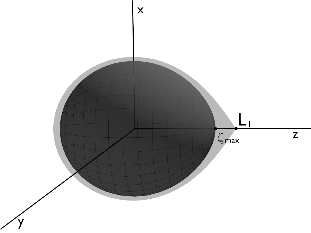
Figure 2: Schematic representation of the primary star with filling factor 0.8. The position of the Lagrange point $L_{1}$is indicated.

We limit ourselves to the case of detached or semi-detached binaries, focusing on one of the stars that we call the primary. Unfortunately, eq. (11) has resisted all our efforts of finding a solution in a closed form forcing us to solve it by numerical integration in the following way.

Let $\zeta$ be the $z$-coordinate of the point at which an equipotential surface $\tilde{\phi}=$const. intersects the axis connecting the two stars, normalised by $a$ the position of the secondary. Its maximum value $\zeta_{\mathrm{max}}$ corresponds to the surface of the primary. If $\zeta_{1}$ is the distance from the centre of the primary to the Lagrange point $L_{1}$ we define the filling factor as $\rho=\zeta_{\mathrm{max}}/\zeta_{1}$ (see Fig. 2). A star with $\rho=1$ fills its Roche lobe. This definition is useful because, apart from normalising constants, the solution depends only on the mass ratio $q$ and the filling factor $\rho$.

As $\zeta$ marks a single equipotential, the potential can be expressed as a function of $\zeta$ only, $\phi=\phi(\zeta)$ and

$$\mathrm{d}\phi=g_{0}(\zeta)\mathrm{d}\zeta=-\@vec{g}_{\mathrm{eff}}\cdot\mathrm{d}\@vec{r}\;,$$ (17)

where $g_{0}(\zeta)=||\@vec{g}_{\mathrm{eff}}(x=0,y=0,z=\zeta)||$.

We can use $\zeta$ as the parameter describing the field line $\mathcal{C}(\theta_{0},\varphi_{0})$ that appears in (11). The differential equation of the field line is given by

$$\@vec{g}_{\mathrm{eff}}\times\mathrm{d}\@vec{r}=\@vec{0}\;.$$ (18)

which expresses that the differential vector is parallel to the effective gravity. Then, using (17) and (18), we can write

$$\frac{\mathrm{d}\@vec{r}}{\mathrm{d}\zeta}=\frac{-g_{0}}{g_{\mathrm{eff}}^{2}}\@vec{g}_{\mathrm{eff}}\;,$$ (19)

from which we can calculate the field line points $\@vec{r}(\zeta,\theta_{0},\varphi_{0})$, for a given starting direction $(\theta_{0},\varphi_{0})$. The line element is

$$\mathrm{d}l=||\mathrm{d}\@vec{r}||=\frac{g_{0}}{g_{\mathrm{eff}}}\mathrm{d}\zeta\;.$$ (20)

Combining (11), (16) and (20), we get the function $f$ which relates the energy flux and the effective gravity. We find

$$f(\theta_{s},\varphi_{s})=f_{0}\exp\left(\int_{0}^{\zeta_{\mathrm{max}}}\frac{2(1+q)}{\left[g_{\mathrm{eff}}(\@vec{r}(\zeta,\theta_{0},\varphi_{0}))\right]^{2}}g_{0}(\zeta)\mathrm{d}\zeta\right)\;.$$ (21)

where $\theta_{s}$ and $\varphi_{s}$ are the coordinates of the point where the field line $\mathcal{C}$ intersects the surface of the primary.

Equations (10) and (19) form a system of four differential equations for solving $f$ that is well-suited for numerical integration. Given an initial direction $(\theta_{0},\varphi_{0})$ and using initial condition (9), the system can be integrated from the centre to the surface. We thus get the value of $f$ at the surface for each $(\theta_{0},\varphi_{0})$ and thus for each $(\theta_{s},\varphi_{s})$. There is a one-to-one correspondance between these coordinates because these field lines do not cross and effective gravity is defined everywhere.

The integration has been performed using the Runge-Kutta-Fehlberg method, often referred to as RKF45, which combines two RK methods of fourth and fifth order Press et al. (2002). It provides an estimate of the truncation error that can be used to adapt the step size.

4 Results

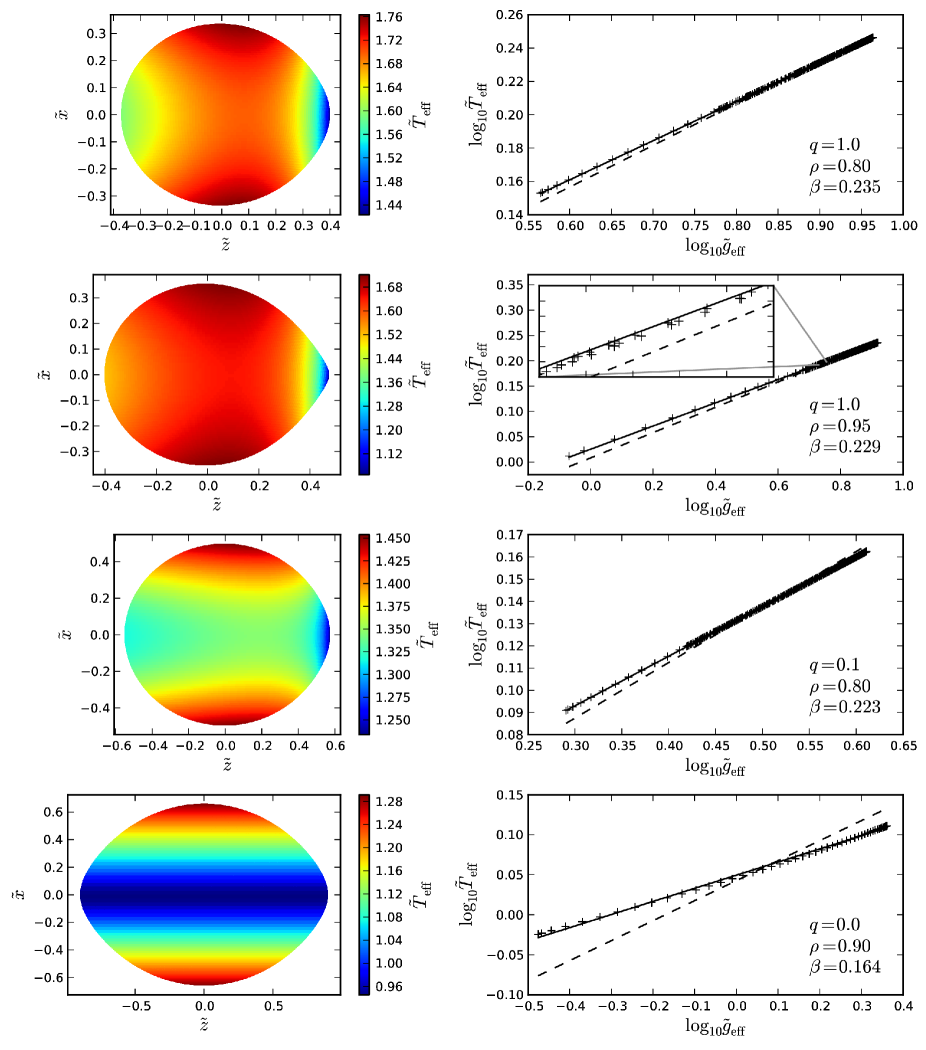
Figure 3: Left: Distribution of $T_{\mathrm{eff}}$ at the surface in one hemisphere of the primary, projected in the plane XZ for several combinations of the mass ratio $q=M_{2}/M_{1}$ and the filling factor $\rho$. Right: Logarithmic plot of $T_{\mathrm{eff}}$ versus $g_{\mathrm{eff}}$ for the same cases. Solid lines are linear fits to the data and the corresponding value of the gravity darkening exponent $\beta$ is indicated in the plots. For comparison, von Zeipel’s law ($\beta=0.25$) is shown by a dashed line. In the second row an inset shows the small dispersion of the points around the fitting power law. The last case ($q=0$) corresponds to an isolated star rotating with angular velocity $\Omega=0.854\Omega_{k}$. Normalised values of effective temperature and gravity are defined in Eq. 22.

Figure 3 shows the results for several combinations of the mass ratio $q$ and filling factor $\rho$. The normalised values of effective temperature and gravity that appear in the figure are defined as

$$\tilde{T}_{\mathrm{eff}}=\left(\frac{4\pi\sigma a^{2}}{L}\right)^{1/4}T_{\mathrm{eff}}\qquad\mbox{and}\qquad\tilde{g}_{\mathrm{eff}}=\frac{a^{2}}{GM_{1}}g_{\mathrm{eff}}\;.$$ (22)

In the left, we can see the distribution of $T_{\mathrm{eff}}$ at the surface in one hemisphere of the star, projected in the plane XZ (remember the definition of the coordinate system shown in Fig. 2). A logarithmic plot of $T_{\mathrm{eff}}$ versus $g_{\mathrm{eff}}$ for each case can be seen on the right. Since the problem has no azimuthal symmetry, the same value of $g_{\mathrm{eff}}$ appears at various places on the surface, but associated with different values of $T_{\mathrm{eff}}$, thus illustrating the absence of a one-to-one relation between $T_{\mathrm{eff}}$ and $g_{\mathrm{eff}}$. However, as shown by the plots, the dispersion is very small (see the inset in Fig. 3). It emphasises a good correlation between the two foregoing quantities. Moreover, the log-log plot shows that this correlation is well approximated by a power law. The actual value of the exponent $\beta$ is always slightly less than 1/4. The worst case is the last one where $q=0$. In fact, this case corresponds to the limit of an isolated star ($M_{2}=0$) rotating at angular velocity

$$\Omega=\rho^{3/2}\Omega_{k}\;,$$ (23)

where $\Omega_{k}$ is the Keplerian angular velocity at the equator $\Omega_{k}=\sqrt{\frac{GM_{1}}{R_{e}^{3}}}$, for which we recover the results obtained in paper I.

Table 1: Fitted values of the gravity darkening exponent $\beta$ in the correlation between $T_{\mathrm{eff}}$ and $g_{\mathrm{eff}}$ as a function of the mass ratio $q=M_{2}/M_{1}$ and the filling factor $\rho$. As the relation does not follow exactly a power law, the maximum relative error in $T_{\mathrm{eff}}$ calculated using the fit compared with the exact value is included in parentheses.

Mass ratio ($q$)	Filling factor ($\rho$)
	$\rho$=0.3	$\rho$=0.5	$\rho$=0.7	$\rho$=0.8	$\rho$=0.9	$\rho$=0.95	$\rho$=0.99
$q$=0.0	0.2456 (0.00004%)	0.2308 (0.0038%)	0.2034 (0.078%)	0.1854 (0.27%)	0.1641 (0.96%)	0.1509 (2.08%)	0.1365 (6.08%)
$q$=0.001	0.2464 (0.00002%)	0.2342 (0.0021%)	0.2110 (0.043%)	0.1958 (0.15%)	0.1789 (0.48%)	0.1708 (0.92%)	0.1666 (1.55%)
$q$=0.01	0.2472 (0.00002%)	0.2374 (0.0013%)	0.2188 (0.025%)	0.2068 (0.090%)	0.1948 (0.31%)	0.1901 (0.56%)	0.1880 (1.31%)
$q$=0.1	0.2482 (0.00004%)	0.2420 (0.0012%)	0.2303 (0.014%)	0.2232 (0.049%)	0.2168 (0.18%)	0.2143 (0.36%)	0.2131 (0.66%)
$q$=1.0	0.2489 (0.00004%)	0.2452 (0.0013%)	0.2385 (0.011%)	0.2346 (0.050%)	0.2308 (0.23%)	0.2291 (0.52%)	0.2280 (1.44%)
$q$=3.0	0.2490 (0.00004%)	0.2455 (0.0015%)	0.2394 (0.020%)	0.2359 (0.092%)	0.2324 (0.37%)	0.2308 (0.80%)	0.2297 (2.18%)
$q$=10.0	0.2489 (0.00005%)	0.2453 (0.0019%)	0.2391 (0.036%)	0.2355 (0.15%)	0.2320 (0.55%)	0.2304 (1.16%)	0.2292 (3.09%)
$q$=100.0	0.2487 (0.00005%)	0.2447 (0.0029%)	0.2377 (0.061%)	0.2337 (0.23%)	0.2298 (0.82%)	0.2279 (1.75%)	0.2267 (4.57%)

In Table 1 we summarize the fitted values of the gravity darkening exponent as a function of $q$ and $\rho$. As pointed out above, the relation between $T_{\mathrm{eff}}$ an $g_{\mathrm{eff}}$ is not exactly a power law so, in order to measure the quality of the fit, we also included, in parentheses, the maximum relative error in $T_{\mathrm{eff}}$ calculated using the fit compared to the exact value. Again, for intermediate $q$, the departures from von Zeipel’s value are moderate, with a value of $\beta$ above $\sim 0.21$ and a correlation between $\log T_{\mathrm{eff}}$ and $\log g_{\mathrm{eff}}$ that remains more or less linear.

The largest deviation is observed for small $q$, for which the effects of nonlinearity are also the strongest. The same behavior can be observed in Fig. 4, where we plot the fitted values of $\beta$ versus the filling factor $\rho$ for different values of $q$. As expected, the asymptotic limit of $\rho=0$, i.e. spherical stars, corresponds to von Zeipel’s value $\beta=1/4$. For a given $\rho$, the maximum value of $\beta$ is attained for $q\sim 3$.

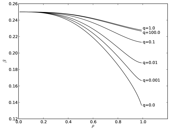
Figure 4: Fitted values of the gravity darkening exponent as a function of the filling factor $\rho$ for different values of the mass ratio $q=M_{2}/M_{1}$. Von Zeipel’s value $\beta=0.25$ is only attained in the limit $\rho=0$ (spherical stars).

5 Conclusions

We have explained in a simple way the old result of Lucy (1967), who derived a gravity darkening law with an exponent $\beta\sim 0.08$ from 1D models of solar-type stars. We trace this value of $\beta$ as a consequence of the boundary conditions used by these stellar models, namely that surface pressure varies like $g/\bar{\kappa}$ and that convective envelopes are close to a $n=3/2$ polytrope.

Noting that 2D or 3D models of rotating or tidally distorted stars cannot be in hydrostatic equilibrium, we argue that the use of gravity darkening exponents derived from 1D models should be avoided. Following paper I, we propose a simple model of the gravity darkening effect that rests on hypothesis generally valid in the envelope of stars:

1. flux is conserved (no heat sources);

2. flux is antiparallel to local effective gravity;

3. gravity is close to that of the Roche model.

These three hypothesis lead to a correlation between effective temperature and effective surface gravity which can be described by a power law with a gravity darkening exponent $\beta$ that weakly depends on mass ratio and Roche lobe filling factor. If we discard extreme mass ratios, $\beta$ remains in the interval $[0.2,0.25]$. It is also independent of the nature (convective or radiative) of the envelope.

This result is interesting to estimate gravity darkening in bright (hot) components of binary stars. It shows that the assumption of the von Zeipel value $\beta=1/4$ is certainly too restrictive.

However, a blind use of this model in binary stars is not recommended either. Indeed, this model does not include:

1. irradiation from the secondary,

2. Coriolis effects on convection,

3. magnetic fields,

4. possible non-synchronism.

The first two effects may indeed invalidate the assumption of the antiparallelism between flux and gravity. Magnetic field may generate spotted regions thus destroying the correlation between effective gravity and flux. Finally, non-synchronism, which may come from differential rotation, alters the assumed shape of the star.

The first three effects may especially affect low-mass companions of binary stars. For these stars, it is likely that the correlation between surface effective gravity and effective temperature is perturbed. The results of Djurašević et al. (2003, 2006) on semi-detached binaries, which give small gravity darkening exponents (namely $\beta\sim 0.1$) for late-type companions, may be viewed as the signature of a weak correlation between $T_{\mathrm{eff}}$ and $g_{\mathrm{eff}}$ for these stars.

In conclusion, the gravity darkening exponent should be interpreted as the parametrization of a correlation between $T_{\mathrm{eff}}$ and $g_{\mathrm{eff}}$. For binary star components, where conditions (a-b-c-d) do not apply, this exponent should be fixed to a value derived from Table 1 according to the mass-ratio of the system and the filling factors of the stars. If one ore more effect of the list exists, clearly a more elaborated model is needed.