The Atacama Cosmology Telescope: Physical Properties of Sunyaev-Zel’dovich Effect clusters on the Celestial Equator

Abstract

We present the optical and X-ray properties of 68 galaxy clusters selected via the Sunyaev-Zel’dovich Effect at 148 GHz by the Atacama Cosmology Telescope (ACT). Our sample, from an area of 504 square degrees centered on the celestial equator, is divided into two regions. The main region uses 270 square degrees of the ACT survey that overlaps with the co-added $ugriz$ imaging from the Sloan Digital Sky Survey (SDSS) over Stripe 82 plus additional near-infrared pointed observations with the Apache Point Observatory 3.5-meter telescope. We confirm a total of 49 clusters to $z\approx 1.3$, of which 22 (all at $z>0.55$) are new discoveries. For the second region the regular-depth SDSS imaging allows us to confirm 19 more clusters up to $z\approx 0.7$, of which 10 systems are new. We present the optical richness, photometric redshifts, and separation between the SZ position and the brightest cluster galaxy (BCG). We find no significant offset between the cluster SZ centroid and BCG location and a weak correlation between optical richness and SZ-derived mass. We also present X-ray fluxes and luminosities from the ROSAT All Sky Survey which confirm that this is a massive sample. One of the newly discovered clusters, ACT-CL J0044.4$+$0113 at $z=1.1$ (photometric), has an integrated XMM-Newton X-ray temperature of $kT_{X}=7.9\pm 1.0$ keV and combined mass of $M_{200a}=8.2_{-2.5}^{+3.3}\times 10^{14}\,h_{70}^{-1}M_{\odot}$ placing it among the most massive and X-ray-hot clusters known at redshifts beyond $z=1$. We also highlight the optically-rich cluster ACT-CL J2327.4$-$0204 (RCS2 2327) at $z=0.705$ (spectroscopic) as the most significant detection of the whole equatorial sample with a Chandra-derived mass of $M_{200a}=1.9_{-0.4}^{+0.6}\times 10^{15}\,h_{70}^{-1}M_{\odot}$, in the ranks of the most massive known clusters like El Gordo and the Bullet Cluster.

1. Introduction

Clusters of galaxies are the cosmic signposts for the largest gravitationally bound objects in the Universe. Their formation and evolution as a function of look-back time provides a measurement of cosmological parameters that complements those obtained from observations of the cosmic microwave background (CMB, e.g., Komatsu et al., 2011; Dunkley et al., 2011; Reichardt et al., 2012), Type Ia Supernovae (e.g., Hicken et al., 2009; Sullivan et al., 2011; Suzuki et al., 2012) and baryon acoustic oscillations (e.g., Percival et al., 2010). The number of clusters as a function of redshift, as demonstrated by X-ray and optically-selected samples (e.g., Vikhlinin et al., 2009; Rozo et al., 2010) provides a strong constraint on both the expansion history of the Universe and the gravitational growth of structure within it (for a recent review see Allen, Evrard, & Mantz, 2011).

The hot gas in galaxy clusters leaves an imprint on the CMB radiation through the Sunyaev-Zel’dovich effect (SZ; Sunyaev & Zeldovich, 1972). The SZ effect has a frequency dependence that produces temperature shifts of the CMB radiation corresponding to a decrement below and an increment above the “null” frequency near 220 GHz (see Birkinshaw, 1999; Carlstrom, Holder, & Reese, 2002, for recent reviews).

Several experiments are now able to carry out large-area cosmological surveys using the SZ effect. The Atacama Cosmology Telescope (ACT) and South Pole Telescope (SPT) are providing samples of galaxy clusters over hundreds of square degrees at all redshifts (Staniszewski et al., 2009; Hincks et al., 2010; Menanteau et al., 2010a; Marriage et al., 2011a; Vanderlinde et al., 2010; Williamson et al., 2011; Reichardt et al., 2012), while the Planck Satellite probes the full sky for clusters up to redshifts of $z\approx 0.55$ (Planck Collaboration et al., 2011a).

Although modest in size, the new SZ cluster samples have proven useful for constraining cosmological parameters (Vanderlinde et al., 2010; Sehgal et al., 2011; Reichardt et al., 2012; Hasselfield et al., 2013) and have opened a new window into the extreme systems, the most massive clusters at high redshift (e.g., Foley et al., 2011; Menanteau et al., 2012), prompting studies that match their observed numbers with the abundance predictions of the standard $\Lambda$CDM cosmology (e.g., Hoyle, Jimenez, & Verde, 2011; Mortonson, Hu, & Huterer, 2011; Waizmann, Ettori, & Moscardini, 2012).

ACT is a millimeter-wave, arcminute-resolution telescope (Fowler et al., 2007; Swetz et al., 2011) designed to observe the CMB on arcminute angular scales (Dünner et al., 2012). The initial set of ACT observations during the 2008 season focused on surveying a 455 deg² region of the southern sky centered near declination -55^∘ (hereafter “the southern strip”). Our previous work studied 23 high-significance clusters from the southern strip (Marriage et al., 2011a) with optical confirmations (Menanteau et al., 2010a). One of the highlights of this previous work was the discovery of the spectacular El Gordo (ACT-CL J0102$-$4915) cluster merger system at $z=0.87$ (Menanteau et al., 2012).

During the 2009 and 2010 seasons, ACT mainly surveyed a long, narrow region of the celestial equator that nearly completely overlaps with the publicly-available optical co-added images from the Sloan Digital Sky Survey (SDSS) of Stripe 82 (hereafter S82; Annis et al., 2011). SDSS provides an immediate optical follow-up of clusters that is of high quality, uniform and at a depth sufficient to detect massive clusters to $z\approx 1$. This is currently unique for high resolution SZ experiments. Furthermore, the uniform SDSS coverage of S82 has allowed combined CMB-optical studies such as the detection of the SZ decrement from low mass (few $10^{14}$ $M_{\odot}$) haloes by stacking Luminous Red Galaxies (LRGs, Hand et al., 2011), the first detection of the kinematic SZ effect (Hand et al., 2012), and the cross-correlation of the ACT CMB lensing convergence maps (Das et al., 2011b) and quasars (Sherwin et al., 2012).

While the number density of SZ-selected clusters is a potentially strong cosmological probe, the confirmation of candidates as true clusters and the determination of their masses is the first and most fundamental step. In this paper we provide the optical and near-infrared (NIR) confirmation of SZ cluster candidates from 504 square degrees of the 148 GHz ACT 2009-2010 maps of the celestial equator. Over the ACT survey area that overlaps S82 (270 deg²) we use the $ugriz$ optical images, supplemented with targeted NIR observations, to identify 49 clusters up to $z\approx 1.3$. For targets outside S82 we use the regular-depth SDSS data from Data Release 8 (DR8; Aihara et al., 2011) to confirm 19 clusters. The contiguous coverage provided by SDSS allows us to investigate potential offsets between the clusters optical and SZ centroid position as well as the relation between optical richness and SZ signal. In a companion paper (Hasselfield et al., 2013) we present a full description of the SZ cluster selection technique as well as cosmological implications using the cluster sample. Recently Reese et al. (2012) presented high-resolution follow-up observations with the Sunyaev-Zel’dovich Array (SZA) for a small sub-sample of the clusters presented here.

Throughout this paper we quote cluster masses as $M_{200a}$ (or $M_{500c}$) which corresponds to the mass enclosed within a radius where the overdensity is 200 (500) times the average (critical) matter density. We assume a standard flat $\Lambda$CDM cosmology with $\Omega_{m}=0.27$ and $\Omega_{\Lambda}=0.73$, and $E(z)=\sqrt{\Omega_{M}(1+z)^{3}+\Omega_{\Lambda}}$. We give relevant quantities in terms of the Hubble parameter $H_{0}=70\,h_{70}$ km s^-1 Mpc^-1. The assumed cosmology has a small effect on the cluster mass, for example if we assume a canonical scaling of $M\propto E(z)^{-1}$, this implies a $2\%-3\%$ increase between $\Omega_{m}=0.27$ and $\Omega_{m}=0.30$ for a flat cosmology at $0.4<z<0.8$. In our analysis we convert masses with respect to average or critical at different overdensities using scalings derived from a Navarro, Frenk, & White (1997, NFW) mass profile and the concentration-mass relation, $c(M,z)$, from simulations (Duffy et al., 2008). All magnitudes are in the SDSS $ugriz$ AB system and all quoted errors are 68% confidence intervals unless otherwise stated.

2. Observations

The detection of cluster candidates was performed from matched-filtered ACT maps at 148 GHz, while confirmation of the clusters was done using a combination of optical and near-infrared (NIR) imaging, and archival ROSAT X-ray data. In the following sections we describe the procedure followed.

2.1. SZ observations

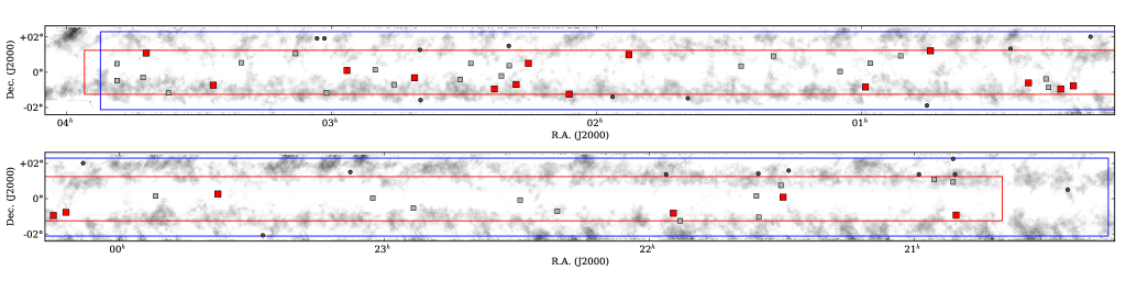
Figure 1.— ACT equatorial survey coverage with the SDSS Stripe 82 deep optical survey region indicated as red box. The red squares are the 18 clusters in the pure sample in S82 (see Section 5.1). Gray squares represent the rest of the confirmed clusters in the S82 region. Circles are other confirmed ACT SZ clusters outside S82. The blue box represents total area ($504$ deg²) covered by ACT.

ACT operates at three frequency bands centered at 148 GHz (2.0 mm), 218 GHz (1.4 mm) and 270 GHz (1.1 mm), each band having a dedicated 1024-element array of transition-edge-sensing bolometers. The 270 GHz band is not as sensitive as the lower frequency channels and the analysis of it is ongoing although not yet complete. ACT has concluded four seasons of observations (2007-2010) surveying two sky areas: the southern strip near declination $-55^{\circ}$ and a region over the celestial equator. In this paper, we apply similar techniques as the ones used on the southern strip for SZ cluster detection and optical identification (Menanteau et al., 2010a; Marriage et al., 2011a) to the ACT 148 GHz equatorial data. A full description of the map making procedure from the ACT time-ordered data is described in Dünner et al. (2012).

Cluster candidates were detected in the 148 GHz ACT equatorial maps over a 504 deg² region bounded by $20^{h}16^{m}<$RA$<3^{h}52^{m}$ and $-2^{\circ}07^{\prime}<$Dec.$<+2^{\circ}18^{\prime}$ as shown in Figure 1 as a blue box over the ACT map (Hasselfield et al., 2013). Nearly fully contained within this region lies the S82 optical imaging area (shown as a red box in Figure 1) which spans $20^{h}40^{m}<$RA$<4^{h}0^{m}$ and $-1^{\circ}15^{\prime}<$Dec.$<+1^{\circ}15^{\prime}$ and covers 275 deg². The effective overlap between the S82 imaging and the ACT maps is 270 deg² and corresponds to the deepest section of the ACT data in the equatorial survey. This constitutes the core of the data we use in this paper to characterize the SZ selection function. In the ACT region of the maps beyond the S82 coverage we use the normal-depth legacy survey from the SDSS DR8. The effective beam for the 148 GHz band for the 2009 and 2010 combined seasons has a FWHM of $1.\!^{\prime}4$.

Here we highlight the principal aspects of the SZ cluster detection procedure described in Hasselfield et al. (2013) to provide context for the characterization of the cluster sample. After subtracting bright sources from the ACT 148 GHz source catalog (corresponding to 1% of the map area), the map is match-filtered in the Fourier domain using a set of signal templates based on the Universal Pressure Profile (UPP) of Arnaud et al. (2010) modeled with a generalized NFW profile (Nagai, Kravtsov, & Vikhlinin, 2007, Appendix A) as a function of physical radius. We use signal templates with FWHM of $0.\!^{\prime}4$ to $9.\!^{\prime}2$ in increments of $0.\!^{\prime}4$ (23 sets) to match-filter the ACT 148 GHz maps to optimize signal-to-noise (S/N) on cluster-shaped objects with an SZ spectral signature. Cluster candidates are identified in the filtered maps as pixels with S/N$>4$ using the core scale in which the cluster was most significantly detected. The catalog of cluster candidates contains positions, central decrements ($\Delta T$), and the local map noise level. Candidates seen at multiple filter scales are cross-identified if the detection positions are within $1^{\prime}$.

2.2. SDSS Optical Data

The main optical data set used for the SZ cluster confirmation is the S82 optical imaging that almost completely overlaps with the deepest region of the ACT equatorial maps with an effective area coverage of 270 deg². ACT’s survey over S82 is unique for high resolution SZ experiments, since it provides immediate optical follow-up of an extremely high and uniform quality at a depth sufficient to detect massive clusters to $z\approx 1$. Beyond this common region we use the shallower single-pass data from DR8 to confidently report cluster identification to $z\approx 0.5$.

The S82 survey is a 275 deg² stripe (represented by the red box in Figure 1) of repeated $ugriz$ imaging centered on the Celestial Equator in the Southern Galactic Cap, as described in Annis et al. (2011). The multi-epoch scanning of the $2^{\circ}\!\!.5$–wide SDSS camera provides between 20 to 40 visits for any given section of the survey which, after aligning and averaging (i.e., co-adding), results in significantly deeper data. The co-added S82 images reach $\sim 2$ magnitudes deeper than the single-pass SDSS data and have a median seeing of $\sim 1.\!\!^{\prime\prime}1$ with a reported 50% completeness for galaxies at $r=23.5$ and $i=23$, while for DR8 this completeness level is reached at $r=21.5$ (Annis et al., 2011). Photometric calibration has typical variation of $0.5\%$ for $griz$ and $1\%-2\%$ for $u$ across the survey. In Figure 2 we show the detection limits for the S82 and DR8 photometry as compared to the observed magnitudes of early-type galaxies of different luminosities at different redshifts.

The co-added, photometrically-calibrated images and catalogs for S82 were released in October 2008 as part of the SDSS Data Release 7 (DR7; Abazajian et al., 2009) and are available at the SDSS Data Archive Server (DAS) and the Catalog Archive Server (CAS), respectively. The co-added data were run through the SDSS pipelines; the standard SDSS flag set is available for all objects.

We retrieved Galactic-extinction-corrected modelMag photometry in all 5 bands for all galaxies from the PhotoObj table designated from runs 106 and 206 under the CAS Stripe82 database to create galaxy catalogs, which we split in $0^{h}20^{m}$ wide tiles in right ascension with no overlap between them to avoid object duplication. As the Stripe82 database does not include spectroscopic information, for each galaxy we used the DR8 CAS database for a spectroscopic redshift, which was ingested into the catalogs if available (Aihara et al., 2011). In order to optimize and speed up our cluster identification we fetched all $ugriz$ fits images for S82 from run numbers 100006 (North) and 200006 (South) and stored them locally to query later. The pixel scale of the co-added images is $0.\!\!^{\prime\prime}396$/pixel for all bands.

We compute photometric redshifts for all objects in the S82 photometric catalog using the spectral-energy-distribution (SED) based Bayesian Photometric Redshift code (BPZ, Benítez, 2000) with no prior. We use the dust-corrected $ugriz$ modelMag magnitudes and the BPZ set of template spectra described in Benítez et al. (2004), which in turn is based on the templates from Coleman et al. (1980) and Kinney et al. (1996). This set consists of El, Sbc, Scd, Im, SB3, and SB2 and represents the typical SEDs of elliptical, early/intermediate-type spiral, late-type spiral, irregular, and two types of starburst galaxies, respectively. For the targets with NIR follow-up observations, the catalogs are augmented by including the $K_{S}$–band imaging. The final results are catalogs with photometric redshifts for all galaxies in S82 augmented by spectroscopic redshifts as available.

For a fraction of the SZ cluster candidates outside the common area between the ACT equatorial maps and S82, we use regular-depth SDSS imaging from DR8 to confirm clusters. We also retrieved $ugriz$ Galactic-extinction-corrected modelMag magnitudes for galaxies, but, unlike for the S82, we only query the DR8 CAS database within a radius of $1^{\circ}$ of each candidate. Similarly we only fetched and combined images from tiles surrounding each candidate to create $10^{\prime}$ fits images in all 5 bands. Given that the DR8 CAS database provides well-tested training-set-based photometric redshifts we do not compute our own SED-based estimates, as we did for S82, and instead we rely on the ones available in the database. In Section 3.2 we discuss the accuracy of the photometric redshift measurements.

2.3. Near Infrared Imaging

Additional pointed follow-up NIR observations with the Near-Infrared Camera and Fabry-Perot Spectrometer (NICFPS) on the ARC 3.5-m telescope of the Apache Point Observatory (APO) aided the confirmation of five high redshift clusters with S/N$>4.7$. These clusters did not have a secure optical cluster counterpart in the deep S82 area. The observations were carried out on UT 2010 Oct 27-28, UT 2011 Nov 02 and UT 2011 Nov 06 when the seeing varied between $0.9-1.\!^{\prime\prime}4$. NICFPS is equipped with a $1024\times 1024$ Hawaii-I RG array with $0.\!^{\prime\prime}273$ pixels and a $4.\!^{\prime}58$ square field of view. We obtained between 1800 – 3870 s of integration in the $K_{S}$ band on each candidate, using 30 s exposures with 8 Fowler samples per exposure (Fowler & Gatley, 1990), in a repeating 5 point dither pattern with box size $20^{\prime\prime}$. The individual exposures were dark subtracted, distortion corrected, flat fielded (using a sky flat made from the science frames), and sky subtracted (using a running median method). SExtractor (Bertin & Arnouts, 1996) was used to produce object masks used in constructing the sky flat and sky images used in the latter two processing steps. The individual exposures were then astrometrically calibrated using SCAMP (Bertin, 2006) and, finally, median combined using SWARP (Bertin et al., 2002). The photometric zero point (on the Vega system) for each image was bootstrapped from the magnitudes of UKIDSS LAS (Lawrence et al., 2007) sources in each field and transformed into the AB system for consistency with the SDSS data. The estimated uncertainty on the zero point spans the range 0.01 – 0.06 mag, with median 0.02 mag. The final images reach $5\sigma$ depth 18.8 – 20.2 mag (median 19.4 mag; measured within a $3^{\prime\prime}$ diameter aperture), estimated by placing 1000 apertures in each image at random positions where objects are not detected. In Table 1 we summarize the NIR observations for the confirmed clusters, which we also discuss in Section 4.1.

For the clusters with NIR imaging, we registered the $K_{S}$ and optical data to create a detection image from the $\chi^{2}$ quadratic sum combination of the $i$ and $K_{S}$–bands using SWARP. Source detection and photometric catalogs were performed using SExtractor (Bertin & Arnouts, 1996) in dual-image mode in which sources were identified on the detection images using a $1.5\sigma$ detection threshold, while magnitudes were extracted at matching locations from all other bands. For clusters with NIR imaging, we use the isophotal magnitudes in the new catalogs to compute photometric redshifts using the same procedure described in Section 3.2, with the only variation being the use of six filters instead of five.

Table 1APO NIR observations of Stripe 82 Clusters

ACT Descriptor	Date Obs.	Exp. Time	photo-z
ACT-CL J0012.0$-$0046	UT 2011, Nov 02	3870 s	$1.36\pm 0.06$
ACT-CL J0044.4$+$0113	UT 2011, Nov 06	3600 s	$1.11\pm 0.03$
ACT-CL J0336.9$-$0110	UT 2010, Oct 27	3600 s	$1.32\pm 0.05$
ACT-CL J0342.0$+$0105	UT 2010, Oct 28	3150 s	$1.07\pm 0.06$
ACT-CL J2351.7$+$0009	UT 2011, Oct 02	1800 s	$0.99\pm 0.03$

2.4. ROSAT X-ray Observations

We extracted X-ray fluxes for all optically confirmed ACT equatorial clusters using the ROSAT All-Sky Survey (RASS) data following the same procedure as in Menanteau & Hughes (2009) and Menanteau et al. (2010a). The raw X-ray photon event lists and exposure maps were downloaded from the MPE ROSAT Archive and were queried with our own custom software. At the ACT SZ position of each cluster, RASS count rates in the $0.5-2$ keV band (corresponding to PI channels 52–201) were extracted from within radii of 3^′ for the source emission and from within a surrounding annulus (5^′ to 25^′ inner and outer radii) for the background emission. The background-subtracted count rates were converted to X-ray luminosity (in the 0.1–2.4 keV band) assuming a thermal spectrum ($kT_{X}=5$ keV) and the Galactic column density of neutral hydrogen ($N_{H}$) appropriate to the source position, using data from the Leiden/Argentine/HI Bonn survey (Kalberla et al., 2005). In Tables 4 and 5 we show the X-ray fluxes and luminosities for all ACT clusters, regardless of the significance of the RASS detection. Uncertainties are estimated from the count rates and represent statistical errors.

3. Analysis and Results

Our analysis provides a sample of optically-confirmed SZ clusters from the ACT cluster candidates at 148 GHz found in the maps on the celestial equator described in Hasselfield et al. (2013). As an important part of this process we measure the “purity” of the ACT SZ candidate population over S82, that is, the fraction of real clusters as a function of SZ detection significance.

3.1. Cluster Confirmation Criteria

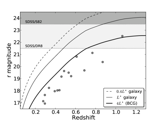
Figure 2.— The observed $r$-band magnitudes of $L^{*}$, $0.4L^{*}$ and $4L^{*}$ (BCG) early-type galaxies as a function of redshift. We use $L^{*}$ as defined Blanton et al. (2003) for the population of red galaxies at $z=0.1$ and allow it to passively evolve with redshift. We show in gray the 50% completeness limits for the SDSS/S82 and DR8 data for galaxies from Annis et al. (2011) reaching $r=23.5$ and $r=21.5$ respectively. For comparison we also show as gray circles the observed $r$-band magnitudes for the BCGs in the SZ southern sample from the imaging reported in Menanteau et al. (2010a).

Our confirmation procedure builds upon our previous work on the ACT southern sample (Menanteau et al., 2010a) and takes advantage of the contiguous and deeper optical coverage available from S82, which allows the systematic and rapid investigation of all SZ cluster candidates, unlike for the 2008 ACT data and associated follow-up. The procedure consists of searching for an optical cluster associated with each candidate’s SZ decrement. This is relatively straightforward, since in concordance $\Lambda$CDM cosmology the halo mass function (e.g., Tinker et al., 2008) predicts that around 90% of massive clusters (i.e., $M_{200a}>3\times 10^{14}\,h_{70}^{-1}M_{\odot}$), such as the ones that make up the current generation of SZ samples, will lie below $z\approx 0.8$ and are therefore accessible for intermediate-depth optical imaging such as in the S82 data set.

The optical confirmation requires the detection of a brightest cluster galaxy (BCG) and an accompanying red sequence of cluster members, which are typically early-type galaxies with luminosities less than $L^{*}$ (the characteristic Schechter luminosity). In Section 3.3 we discuss our richness criterion for optical confirmation of the sample. We use the completeness limits estimated from simulations by Annis et al. (2011) to determine how far in redshift we can “see” massive clusters in S82. For this, we compare the completeness limits of S82 observations to the expected and observed apparent magnitudes of galaxies in clusters as a function of redshift. We estimated the expected apparent galaxy $r$-band magnitude as a function of redshift using $L^{*}$ as defined for the population of red galaxies by Blanton et al. (2003) at $z=0.1$ and allowing passive evolution according to a solar metallicity Bruzual & Charlot (2003) $\tau=1.0$ Gyr burst model formed at $z_{f}=5$. We show this relation in Figure 2 for a range of luminosities ($0.4L^{*}$, $L^{*}$ and $4L^{*}$) aimed at representing the cluster members from the faint ones to the BCG. We also show as different gray levels the 50% completeness level as determined by the simulations for the S82 and DR8 samples (Annis et al., 2011). Figure 2 also shows, for comparison, the apparent $r$-band magnitude of BCGs in the ACT southern cluster sample Menanteau et al. (2010a).

We conclude that we can comfortably detect cluster BCGs in S82 up to $z>1$ and outside S82 to $z=0.7$. A cluster red sequence will be confidently detected to somewhat lower redshifts, $z\approx 0.8$ (S82) and $z\approx 0.5$ (outside S82), thus satisfying our criteria for optical cluster confirmation. In summary, we search for a BCG and associated red-sequence around each SZ candidate; if this condition is satisfied, we estimate the redshift and richness for the cluster. If the cluster richness satisfies the minimum richness criteria (see Section 3.3) we list the candidate as a real cluster.

3.2. Cluster Redshift Determination

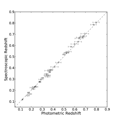
Figure 3.— Spectroscopic redshift versus photometric redshift for the sub-sample 37 of ACT equatorial clusters with known spectroscopic redshifts. Circles represent clusters from the S82 area while squares are system outside the S82 area. Error bars show the 68% C.L. uncertainties on the cluster photometric redshift.

In practice we perform the cluster confirmation by working on $10^{\prime}\times 10^{\prime}$ wide images centered on the position of the SZ candidate that are created from stitching together nearby S82 tiles in all 5 SDSS bands. Our inspection relies on a custom-created automated software that enables us to interactively search for a BCG and its red cluster sequence using our own implementation of the MaxBCG cluster finder (Koester et al., 2007) algorithm, as described in Menanteau et al. (2010b) for the Southern Cosmology Survey (SCS; Menanteau et al., 2009). Although our implementation of the MaxBCG cluster algorithm represents our best effort to replicate the method as described in Koester et al. (2007), the measured richness values should not be expected to be exactly as in the original MaxBCG implementation due to slight differences in the handling of photometric errors and background subtraction. This consists of visually selecting the BCG and from that recorded position iteratively choosing cluster member galaxies using the photometric redshifts and a $3\sigma$ clipping algorithm within a local self-defined color-magnitude relation. For candidates with APO $K_{S}$ follow-up imaging we use 6 bands, which are limited to the $\sim 5^{\prime}\times 5^{\prime}$ field-of-view (FOV) of NICFPS, but otherwise the procedure is the same. Our software aids the precise determination of the BCG by visually flagging all early-type galaxies (i.e., galaxies SED types 0 and 1 from BPZ) that are more luminous than $4L^{*}$ galaxies, with $L^{*}$ as defined above. Once the BCG has been established, the next step in the optical confirmation is to define the cluster redshift and color criteria to be used in selecting cluster members as these are required to estimate the richness of the cluster.

The determination of the cluster redshift is an iterative process, using our custom-developed tools, that starts with the redshift of the BCG as the initial guess for the cluster’s redshift and center. It then estimates the redshift as the mean value of the $N$ brightest early-type galaxies (with $N=7$) within an inner radius of $250\,h^{-1}$kpc (with $H_{0}=100{\rm\,km\,s^{-1}\,Mpc^{-1}}\,h$ as defined by MaxBCG) and the redshift interval $\Delta z=0.045(1+z_{c})$ where $z_{c}$ is the redshift of the cluster. For redshift determination we use the $N$ brightest early-type galaxies, rather than the BCG alone, to mitigate against biased photometric redshifts resulting from BCGs with peculiar colors, such as in cool core clusters. The new redshift is used as input and the same procedure is repeated until convergence on the redshift value is achieved, which usually occurs in three iterations or less. The selection of $N=7$ was informed by optimizing cluster redshifts for systems with known spectroscopic redshifts. Uncertainties in the cluster redshifts are determined via bootstrap resampling (10,000 times) of the galaxies selected for the redshift determination. We also explored estimating errors using Monte Carlo realizations of the sample which provided similar results. We note that although our catalogs contain the spectroscopic redshifts available from SDSS, in the procedure described here we only make use of the photometric redshifts, in order to make a direct comparison with the spectroscopic information.

Another important advantage of the overlap of ACT with S82 and SDSS is that for all clusters at $z<0.3$ the BCG was spectroscopically targeted by SDSS and has a spectroscopic redshift. Moreover, as BCGs are very luminous objects, in several cases it was possible to match them with a spectroscopic redshift from SDSS to $z\approx 0.5$. There are 25 ACT clusters in S82 for which a spectroscopic redshift was available from SDSS for the BCG or the next brightest galaxy in the cluster. For the ACT area outside S82, the CAS DR8 database provides imaging but no spectroscopic redshifts are available from SDSS on this region. Additionally, within the sample presented in this paper, 21 (18 are on S82) S/N$>4.5$ SZ clusters have multi-object spectroscopic follow-up observations using GMOS on Gemini-S as part of our program aimed at obtaining dynamical masses for ACT clusters at $z>0.35$ (Sifón et al., 2012). The observations were carried out as part of our ongoing programs (GS-2011B-C-1, GS-2012A-C-2 and GS-2012B-C-3) and processed using our custom set of tools as described in Sifón et al. (2012). The full description of the ACT equatorial sample follow-up with Gemini will be described in a future paper (Sifón et al., in prep.). In Figure 3 we show that the photometric and spectroscopic redshifts are in good agreement. Thus for clusters without spectroscopic redshifts, up to $z\approx 0.8$, we confirm that our photometric ones will be quite accurate. For clusters at $z>0.9$, due to the lack of spectroscopic redshifts, we can only assume that the SDSS well-calibrated photometry provides robust estimates. Both photometric and spectroscopic redshifts for the full cluster sample are given in Tables 2 and 3.

3.3. Defining Cluster Membership

In order to have a richness measurement useful to compare across the SZ cluster sample, one must define cluster membership. We follow a similar procedure to that in Menanteau et al. (2010b). Once the redshift of the cluster is determined, we use BPZ-defined early-type galaxies within the same $250\,h^{-1}$kpc radius and redshift interval $\Delta z=0.045(1+z_{c})$ as above to obtain a local self-defined color-magnitude relation (CMR) for each color combination, $g-r$, $r-i$, and $i-z$ ($z-K_{s}$ when available) for all cluster members, using a $3\sigma$ clipping algorithm. For the determination of cluster members we use the spectroscopic redshift when available to define $z_{c}$. We use these spatial and color criteria to determine $N_{\rm 1Mpc}$, the number of galaxies within $1h^{-1}$ Mpc of the cluster center as defined by Koester et al. (2007). Formally, we compute $N_{\rm gal}=N_{\rm 1Mpc}$ by including those galaxies within a projected $1h^{-1}$ Mpc from the cluster center and within $\Delta z=0.045(1+z_{c})$ that satisfy three conditions: (1) the galaxy must have the SED of an early type according to BPZ, (2) it must have the appropriate color to be a cluster member (i.e., colors within $3\sigma$ of the local CMR for all color combinations) and (3) it must have the right luminosity, dimmer than the BCG and brighter than $0.4L^{*}$. Additionally we designate cluster members according to the estimated cluster size $R_{200}$, defined as the radius at which the cluster galaxy density is $200\Omega_{m}^{-1}$ times the mean space density of galaxies in the present Universe. We estimated the scaled radius $R_{200}$ using the empirical relation from Hansen et al. (2005), $R_{200}=0.156N_{\rm 1Mpc}^{0.6}h^{-1}$Mpc which is derived from the SDSS. Hence $N_{200}$ is the number of galaxies satisfying the above conditions within $R_{200}$. We note however, that our ability to uniformly select cluster members to $0.4L^{*}$ depends on the imaging depth of the data available. From Figure 2 we infer that we can detect $0.4L^{*}$ galaxies to $z\approx 0.6$ and $z\approx 0.4$ for clusters inside and outside of S82 region respectively. Beyond this redshift range our richness values underestimate the true values. We caution the reader that beyond this redshift range our richness values underestimate the true values as we do not attempt to correct for the incompleteness of detecting galaxies expected above $0.4L^{*}$ at our limiting magnitude.

For our richness measurements we estimated the galaxy background contamination and implemented an appropriate background subtraction method following the same procedure described in Menanteau et al. (2009) (see section 3.1). We use a statistical removal of unrelated field galaxies with similar colors and redshifts that were projected along the line of sight to each cluster. We estimate the surface number density of ellipticals in an annulus surrounding the cluster (within $4<r<9\,h^{-1}$Mpc) with the same $\Delta z$ as above and the same colors as the cluster members. We measure this background contribution around the outskirts of each cluster and obtain a corrected value $N_{\rm gal}$ which is used to compute $R_{200}$ and then a corresponding value of $N_{200}$. The magnitude of the correction ranges between $10\%-40$% depending on the cluster richness. For the clusters confirmed using APO observations, the smaller FOV of NICFPS precludes us from making a proper background correction for the $N_{\rm gal}$ estimate. Instead we choose a conservative 40% correction factor. In the few cases where the cluster is located near the edge of the optical coverage of S82 and the projected area of a $1h^{-1}$ Mpc aperture is not fully contained within the optical data we scale up $N_{\rm gal}$ by the fraction of the missing area. We will refer to the corrected values hereafter.

The measured richness value, $N_{\rm gal}$, was used in addition to the presence of a BCG and accompanying red sequence to optically confirm cluster candidates; we require a numerical value of $N_{\rm gal}>15$. In practice this additional constraint resulted in the removal of only one candidate. In Tables 2 and 3 we present the $N_{\rm gal}$ estimated for the S82 and DR8 sample respectively.

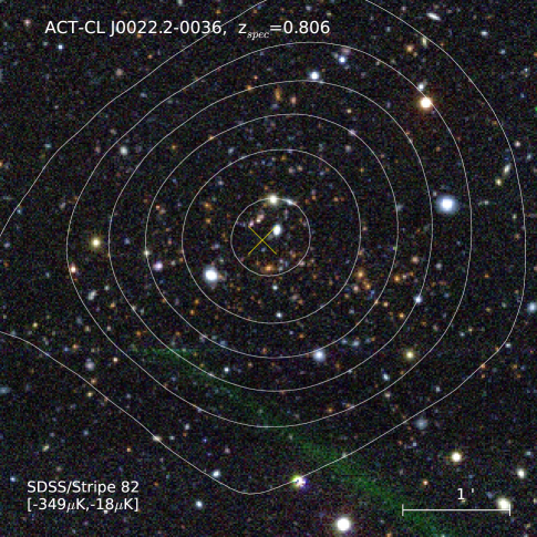
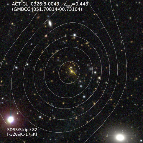
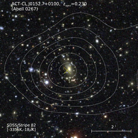
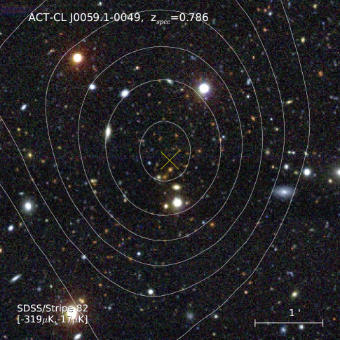
Figure 4.— Composite color images for 4 ACT SZ clusters optically confirmed using the S82 imaging. The horizontal bar shows the scale of the images, where north is up and east is left. White contours show the 148 GHz SZ maps with the minimum and maximum levels, in $\mu$K, displayed between brackets. The yellow cross shows the location of the centroid of the SZ detection.

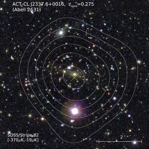
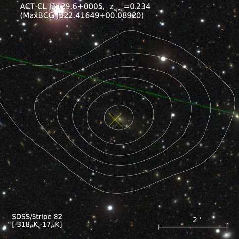
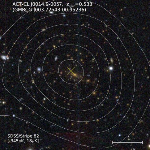
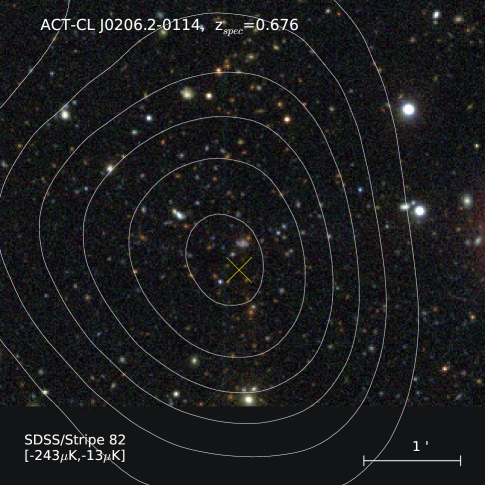
Figure 5.— Composite color images for 4 ACT SZ clusters optically confirmed using the S82 imaging. The horizontal bar shows the scale of the images, where north is up and east is left. White contours show the 148 GHz SZ maps with the minimum and maximum levels, in $\mu$K, displayed between brackets. The yellow cross shows the location of the centroid of the SZ detection.

4. The ACT Equatorial SZ Cluster Sample

Our optical confirmation of SZ candidates has resulted in a new sample of 68 clusters: 49 systems are located in the area overlapping with S82 and 19 clusters on the area that overlaps with the shallower DR8 data.

Table 2Optically confirmed ACT Equatorial clusters on Stripe 82

ACT Descriptor	R.A. (J2000)	Dec. (J2000)	$z$-spec	$z$-photo	$N_{\rm gal}$	SNR	BCG distance	Alternative Name
					($1h^{-1}$ Mpc)	(148 GHz)	(Mpc $h_{70}^{-1}$)
ACT-CL J0022.2$-$0036	00:22:13.0	$-$00:36:33.8	0.805	$0.80\pm 0.03$	$65.9\pm 8.1^{\ast}$	9.8	0.124
ACT-CL J0326.8$-$0043	03:26:49.9	$-$00:43:51.7	0.448	$0.45\pm 0.03$	$41.7\pm 6.5$	9.1	0.014	GMBCG J051.70814-00.73104
ACT-CL J0152.7$+$0100	01:52:41.9	$+$01:00:25.5	0.230	$0.23\pm 0.02$	$67.2\pm 8.2$	9.0	0.026	Abell 0267
ACT-CL J0059.1$-$0049	00:59:08.5	$-$00:50:05.7	0.786	$0.77\pm 0.03$	$41.0\pm 6.4^{\ast}$	8.4	0.064
ACT-CL J2337.6$+$0016	23:37:39.7	$+$00:16:16.9	0.275	$0.28\pm 0.01$	$57.8\pm 7.6$	8.2	0.036	Abell 2631
ACT-CL J2129.6$+$0005	21:29:39.9	$+$00:05:21.1	0.234	$0.24\pm 0.01$	$35.0\pm 5.9$	8.0	0.028	RX J2129.6+0005
ACT-CL J0014.9$-$0057	00:14:54.1	$-$00:57:08.4	0.533	$0.52\pm 0.02$	$56.2\pm 7.5$	7.8	0.070	GMBCG J003.72543-00.95236
ACT-CL J0206.2$-$0114	02:06:13.4	$-$01:14:17.0	0.676	$0.68\pm 0.02$	$68.4\pm 9.5^{\ast}$	6.9	0.123
ACT-CL J0342.0$+$0105	03:42:02.1	$+$01:05:07.5	$\cdots$	$1.07\pm 0.06$	$41.2\pm 6.3^{\ast}$	5.9	0.248
ACT-CL J2154.5$-$0049	21:54:32.3	$-$00:49:00.4	0.488	$0.48\pm 0.02$	$56.9\pm 7.5$	5.9	0.090	WHL J215432.2-004905
ACT-CL J0218.2$-$0041	02:18:16.8	$-$00:41:41.8	0.672	$0.65\pm 0.03$	$39.2\pm 6.3^{\ast}$	5.8	0.262
ACT-CL J0223.1$-$0056	02:23:10.0	$-$00:57:08.9	0.663	$0.64\pm 0.04$	$50.5\pm 7.1^{\ast}$	5.8	0.159	in GMB2011
ACT-CL J2050.5$-$0055	20:50:29.7	$-$00:55:40.6	0.622	$0.60\pm 0.03$	$38.6\pm 6.2^{\ast}$	5.6	0.098	in GMB2011
ACT-CL J0044.4$+$0113	00:44:25.6	$+$01:12:48.7	$\cdots$	$1.11\pm 0.03$	$73.0\pm 8.5^{\ast}$	5.5	0.258
ACT-CL J0215.4$+$0030	02:15:28.5	$+$00:30:37.3	0.865	$0.73\pm 0.03$	$29.5\pm 3.8^{\ast}$	5.5	0.046
ACT-CL J0256.5$+$0006	02:56:33.7	$+$00:06:28.8	0.363	$0.37\pm 0.01$	$39.8\pm 6.3$	5.4	0.113	RX J0256.5+0006
ACT-CL J0012.0$-$0046	00:12:01.8	$-$00:46:34.5	$\cdots$	$1.36\pm 0.06$	$29.2\pm 5.3^{\ast}$	5.3	0.313
ACT-CL J0241.2$-$0018	02:41:15.4	$-$00:18:41.0	0.684	$0.68\pm 0.03$	$50.5\pm 7.1^{\ast}$	5.1	0.040
ACT-CL J0127.2$+$0020	01:27:16.6	$+$00:20:40.9	0.379	$0.37\pm 0.02$	$64.8\pm 8.1$	5.1	0.075	GMBCG J021.81939+00.34469
ACT-CL J0348.6$+$0029	03:48:36.7	$+$00:29:33.0	0.297	$0.29\pm 0.02$	$29.4\pm 5.4$	5.0	0.142	GMBCG J057.17821+00.48718
ACT-CL J0119.9$+$0055	01:19:58.1	$+$00:55:33.6	$\cdots$	$0.72\pm 0.03$	$21.5\pm 3.3^{\ast}$	5.0	0.218
ACT-CL J0058.0$+$0030	00:58:05.7	$+$00:30:58.1	$\cdots$	$0.76\pm 0.02$	$47.0\pm 6.8^{\ast}$	5.0	0.199
ACT-CL J0320.4$+$0032	03:20:29.7	$+$00:31:53.7	0.384	$0.38\pm 0.02$	$55.9\pm 7.5$	4.9	0.158	GMBCG J050.12410+00.53157
ACT-CL J2302.5$+$0002	23:02:35.0	$+$00:02:34.2	0.520	$0.50\pm 0.01$	$61.4\pm 7.8$	4.9	0.080	GMBCG J345.64608+00.04281
ACT-CL J2055.4$+$0105	20:55:23.2	$+$01:06:07.5	0.408	$0.41\pm 0.03$	$37.7\pm 6.1$	4.9	0.233	GMBCG J313.84687+01.10212
ACT-CL J0308.1$+$0103	03:08:12.1	$+$01:03:15.0	0.633	$0.63\pm 0.03$	$41.1\pm 6.4^{\ast}$	4.8	0.174
ACT-CL J0336.9$-$0110	03:36:57.1	$-$01:09:48.3	$\cdots$	$1.32\pm 0.05$	$29.1\pm 5.1^{\ast}$	4.8	0.277
ACT-CL J0219.8$+$0022	02:19:50.4	$+$00:22:14.9	0.537	$0.53\pm 0.02$	$59.0\pm 7.7$	4.7	0.191	GMBCG J034.95781+00.37385
ACT-CL J0348.6$-$0028	03:48:39.5	$-$00:28:16.9	0.345	$0.34\pm 0.02$	$56.9\pm 7.5$	4.7	0.095	GMBCG J057.14850-00.43348
ACT-CL J2351.7$+$0009	23:51:44.6	$+$00:09:16.2	$\cdots$	$0.99\pm 0.03$	$76.0\pm 8.7^{\ast}$	4.7	0.039
ACT-CL J0342.7$-$0017	03:42:42.6	$-$00:17:08.3	0.310	$0.30\pm 0.01$	$36.3\pm 6.0$	4.6	0.132	GMBCG J055.67773-00.28564
ACT-CL J0250.1$+$0008	02:50:08.4	$+$00:08:16.4	$\cdots$	$0.78\pm 0.03$	$32.7\pm 5.7^{\ast}$	4.5	0.084
ACT-CL J2152.9$-$0114	21:52:55.6	$-$01:14:53.2	$\cdots$	$0.69\pm 0.02$	$22.7\pm 3.9^{\ast}$	4.4	0.156
ACT-CL J2130.1$+$0045	21:30:08.8	$+$00:46:48.3	$\cdots$	$0.71\pm 0.04$	$21.5\pm 3.3^{\ast}$	4.4	0.554
ACT-CL J0018.2$-$0022	00:18:18.4	$-$00:22:45.8	$\cdots$	$0.75\pm 0.04$	$27.8\pm 5.3^{\ast}$	4.4	0.393
ACT-CL J0104.8$+$0002	01:04:55.3	$+$00:03:36.2	0.277	$0.28\pm 0.00$	$64.4\pm 8.0$	4.3	0.235	MaxBCG J016.23069+00.06007
ACT-CL J0017.6$-$0051	00:17:37.6	$-$00:52:42.0	0.211	$0.22\pm 0.01$	$38.3\pm 6.2$	4.2	0.268	MaxBCG J004.40671-00.87833
ACT-CL J0230.9$-$0024	02:30:53.8	$-$00:24:40.9	$\cdots$	$0.44\pm 0.03$	$19.9\pm 4.5$	4.2	0.158	WHL J023055.3-002549
ACT-CL J0301.1$-$0110	03:01:12.0	$-$01:10:47.7	$\cdots$	$0.53\pm 0.04$	$24.5\pm 5.0$	4.2	0.260	in GMB2011
ACT-CL J0051.1$+$0055	00:51:12.8	$+$00:55:54.4	$\cdots$	$0.69\pm 0.03$	$20.5\pm 3.2^{\ast}$	4.2	0.417
ACT-CL J0245.8$-$0042	02:45:51.7	$-$00:42:16.4	0.179	$0.17\pm 0.01$	$40.2\pm 6.3$	4.1	0.038	Abell 0381
ACT-CL J2051.1$+$0056	20:51:11.0	$+$00:56:46.1	0.333	$0.35\pm 0.01$	$20.2\pm 4.5$	4.1	0.066	GMBCG J312.79620+00.94615
ACT-CL J2135.1$-$0102	21:35:12.0	$-$01:03:00.1	$\cdots$	$0.33\pm 0.01$	$68.0\pm 8.2$	4.1	0.242	GMBCG J323.80039-01.04962
ACT-CL J0228.5$+$0030	02:28:30.4	$+$00:30:35.7	$\cdots$	$0.72\pm 0.02$	$31.5\pm 4.0^{\ast}$	4.0	0.182
ACT-CL J2229.2$-$0004	22:29:07.5	$-$00:04:11.0	$\cdots$	$0.61\pm 0.05$	$16.4\pm 3.9^{\ast}$	4.0	0.569
ACT-CL J2135.7$+$0009	21:35:39.5	$+$00:09:57.1	0.118	$0.12\pm 0.00$	$75.3\pm 8.7$	4.0	0.144	Abell 2356
ACT-CL J2253.3$-$0031	22:53:24.2	$-$00:30:30.8	$\cdots$	$0.54\pm 0.01$	$23.0\pm 3.4$	4.0	0.488
ACT-CL J2220.7$-$0042	22:20:47.0	$-$00:41:54.4	$\cdots$	$0.57\pm 0.03$	$34.5\pm 5.9$	4.0	0.277	in GMB2011
ACT-CL J0221.5$-$0012	02:21:36.6	$-$00:12:19.8	0.589	$0.57\pm 0.03$	$21.2\pm 4.6$	4.0	0.246	in GMB2011

Note. — R.A. and Dec. positions denote the BCG location in the optical images of the cluster from our confirmation procedure. . The SZ position was used to construct the ACT descriptor identifiers. Spectroscopic redshifts are reported when available and come from the DR8 spectroscopic database and our own follow-up with GMOS on Gemini South. The horizontal line denotes the demarcation for the SZ cluster sample with 100% purity. Values of S/N are from Hasselfield et al. (2013).

4.1. Clusters in Stripe 82

In Table 2 we present the 49 clusters in the 270 deg² area in S82 along with their redshift information, BCG positions and optical richness. In Figures 4 and 5 we show 8 examples of $z<1$ clusters confirmed using the S82 imaging alone, while in Figure 6 we show examples of clusters confirmed using the additional $K_{S}$-band APO imaging. Optical and NIR images for the full sample are available at http://peumo.rutgers.edu/act/S82. We used NED to search for cluster counterparts for our sample using a $500\,h_{70}^{-1}$kpc matching radius and found that a number of them are well-known $z<0.35$ clusters reported as part of the Abell (Abell, 1958), ROSAT All-Sky Galaxy Cluster Survey (NORAS; Böhringer et al., 2000) and MaxBCG (Koester et al., 2007) catalogs. Also using NED we found matches for $z<0.55$ systems in the GMBCG (Hao et al., 2010) and WHL (Wen, Han, & Liu, 2009) optical cluster catalogs. The GMBCG catalog is an improved version of the MaxBCG method which used the SDSS DR7. In Table 2 we designate the first reported alternative name for each system. For higher redshift systems we compared our sample with the catalog from Geach, Murphy, & Bower (2011, GMB2011) which uses a cluster red sequence algorithm on the same deep co-added S82 data used in this analysis to detect clusters. We searched for counterparts using the same match radius and found 5 previously reported GMB2011 systems at $0.50<z<0.65$. Beyond $z>0.65$ all SZ confirmed cluster in S82 represent new discoveries, highlighting the power of the SZ effect to discover massive galaxy clusters at high redshift. In summary, of the 49 ACT SZ-selected clusters from S82, 22 are new and lie at $z>0.54$.

Our APO follow-up campaign aided in the confirmation of five new clusters at $z\geq 1$ over the S82 region by the addition of the $K_{S}$ imaging, described in Section 2.3, to the 5 optical bands. In Figures 6 and 7 we show the optical and NIR composite images of the 5 clusters at $z\geq 1$. In Table 1 we present a summary for the 5 new clusters confirmed with the help of the NIR imaging.

4.2. Additional Clusters Outside Stripe 82

In Table 3 we present the sample of 19 optically confirmed clusters using the $ugriz$ imaging from the SDSS DR8 where we provide the same information as for the S82 sample above. The shallower coverage over the area beyond S82 only allows us to present optical confirmations for an incomplete subsample. As we see from Figure 2, the imaging depth of the DR8 data set can only “see” $L^{*}$ galaxies up to $z\approx 0.5$. Moreover, the DR8 footprint does not fully cover the ACT equatorial region. Within this sky region, which contains 10 new clusters, is located the most significant SZ detection of the whole ACT equatorial sample, ACT-CL J2327.4$-$0204 which we discuss in detail in Section 4.3.2.

An approved dedicated optical and NIR follow-up program using the SOAR 4.1-m and APO 3.5-m telescopes in 2012B will provide a more uniform and complete cluster sample for the remaining area outside S82.

Table 3Optically confirmed ACT Equatorial clusters outside Stripe 82, with DR8 coverage

ACT Descriptor	R.A. (J2000)	Dec. (J2000)	$z$-spec	$z$-photo	$N_{\rm gal}$	SNR	BCG distance	Alternative Name
					($1h^{-1}$ Mpc)	(148 GHz)	(Mpc $h_{70}^{-1}$)
ACT-CL J2327.4$-$0204	23:27:27.6	$-$02:04:37.4	0.705	$0.69\pm 0.04$	$61.7\pm 7.9^{\ast}$	13.1	0.028	RCS2 2327
ACT-CL J2135.2$+$0125	21:35:18.7	$+$01:25:27.0	0.231	$0.25\pm 0.01$	$57.6\pm 7.6$	9.3	0.184	Abell 2355
ACT-CL J0239.8$-$0134	02:39:53.1	$-$01:34:56.0	0.375	$0.35\pm 0.03$	$84.0\pm 9.2$	8.8	0.121	Abell 0370
ACT-CL J2058.8$+$0123	20:58:58.0	$+$01:22:22.2	$\cdots$	$0.32\pm 0.02$	$76.9\pm 8.8$	8.3	0.361
ACT-CL J0045.2$-$0152	00:45:12.5	$-$01:52:31.6	0.545	$0.55\pm 0.02$	$53.5\pm 7.3^{\ast}$	7.5	0.182
ACT-CL J2050.7$+$0123	20:50:43.1	$+$01:23:29.2	0.333	$0.35\pm 0.03$	$56.5\pm 7.5$	7.4	0.104	RXC J2050.7+0123
ACT-CL J2128.4$+$0135	21:28:23.4	$+$01:35:36.4	0.385	$0.39\pm 0.03$	$87.2\pm 9.3$	7.3	0.165
ACT-CL J2025.2$+$0030	20:25:12.7	$+$00:31:33.8	$\cdots$	$0.34\pm 0.02$	$56.6\pm 7.5$	6.4	0.235
ACT-CL J0026.2$+$0120	00:26:15.9	$+$01:20:37.0	$\cdots$	$0.65\pm 0.04$	$33.6\pm 5.8^{\ast}$	6.3	0.196
ACT-CL J2307.6$+$0130	23:07:39.9	$+$01:30:55.8	$\cdots$	$0.36\pm 0.02$	$75.5\pm 8.7$	6.1	0.027	ZwCl 2305.0+0114
ACT-CL J2156.1$+$0123	21:56:08.5	$+$01:23:27.3	0.224	$0.21\pm 0.02$	$64.9\pm 8.1$	6.0	0.094	Abell 2397
ACT-CL J0301.6$+$0155	03:01:38.2	$+$01:55:14.6	0.167	$0.19\pm 0.01$	$49.4\pm 7.0$	5.8	0.069	RXC J0301.6+0155
ACT-CL J2051.1$+$0215	20:51:12.2	$+$02:15:58.3	0.321	$0.35\pm 0.02$	$56.4\pm 7.5$	5.2	0.221	RXC J2051.1+0216
ACT-CL J0303.3$+$0155	03:03:21.1	$+$01:55:34.5	0.153	$0.17\pm 0.01$	$26.1\pm 5.1$	5.2	0.060	Abell 0409
ACT-CL J0156.4$-$0123	01:56:24.3	$-$01:23:17.3	$\cdots$	$0.45\pm 0.04$	$37.9\pm 6.2^{\ast}$	5.2	0.011
ACT-CL J0219.9$+$0129	02:19:52.1	$+$01:29:52.2	$\cdots$	$0.35\pm 0.02$	$66.0\pm 8.1$	4.9	0.154
ACT-CL J0240.0$+$0116	02:40:01.7	$+$01:16:06.4	$\cdots$	$0.62\pm 0.03$	$31.9\pm 5.7^{\ast}$	4.8	0.077
ACT-CL J0008.1$+$0201	00:08:10.4	$+$02:01:12.3	$\cdots$	$0.36\pm 0.04$	$44.8\pm 6.7$	4.7	0.028
ACT-CL J0139.3$-$0128	01:39:16.7	$-$01:28:45.2	$\cdots$	$0.70\pm 0.03$	$26.9\pm 5.2^{\ast}$	4.3	0.549

Note. — R.A. and Dec. positions denote the BCG location in the optical images of the cluster from our confirmation procedure. The SZ position was used to construct the ACT descriptor identifiers. Spectroscopic redshifts are reported when available and come from the DR8 spectroscopic database and our own follow-up with GMOS on Gemini South. Values of S/N are from Hasselfield et al. (2013).

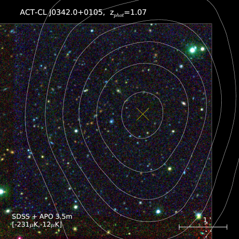
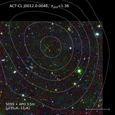
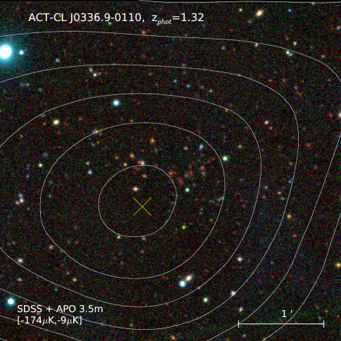
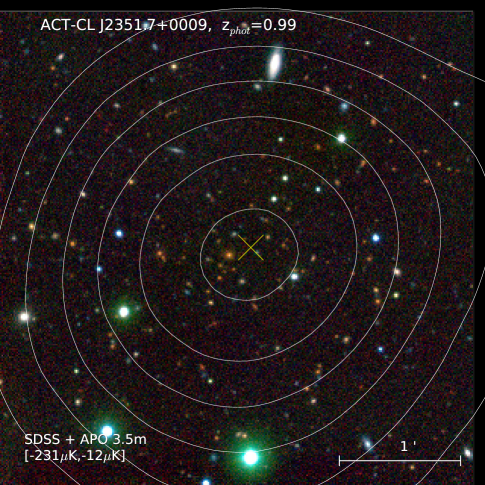
Figure 6.— Composite color images for 4 of the 5 high redshift ACT SZ clusters confirmed using optical (S82) and near-infrared (APO) imaging. The horizontal bar shows the scale of the images, where north is up and east is left. White contours show the 148 GHz SZ maps with the minimum and maximum levels, in $\mu$K, displayed between brackets. The yellow cross shows the location of the centroid of the SZ detection.

4.3. Notable Clusters

In the following sections we provide detailed information on a selected few individual clusters that are worthy of special attention.

4.3.1 ACT-CL J0044.4$+$0113

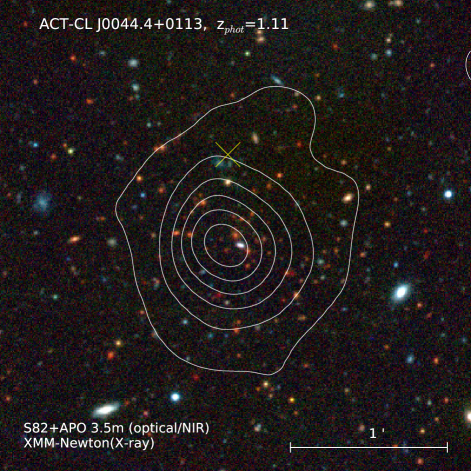
Figure 7.— The XMM-Newton archival X-ray observations (contours) that serendipitously contain ACT-CL J0044.4$+$0113 overlaid on the composite optical (S82) and NIR (APO) pseudo-color image. The X-ray observations show its extended nature with a best fit temperature of $kT_{X}=7.9\pm 1.0$ keV for the photometric redshift of $z=1.11$.

ACT-CL J0044.4$+$0113 appeared serendipitously in an archival XMM-Newton observation targeting the SLAC lens object SDSSJ0044+0113 (Auger et al., 2009) taken on Jan 10, 2010 (PI:Treu, ObsID:0602340101). After flare rejection we obtained exposure times of 21 ks for each MOS and 15 ks for the pn. Our analysis used SAS version 12.0.1. In Figure 7 we show the composite optical/NIR color image for ACT-CL J0044.4$+$0113 with the overplotted XMM-Newton X-ray surface brightness contours in the 0.5-4.5 keV band shown in white. The cluster is clearly extended and the X-ray surface brightness is above background up to a radius of $\sim$50^′′ (439 $h_{70}^{-1}$ kpc). Fits to the integrated spectrum to $R_{500c}$ from a region of radius $1\!^{\prime}.5$, using a local annular region (covering 2.1^′ to 4.2^′) results in a best fit gas temperature of $kT_{X}=7.9\pm 1.0$ keV and 0.5–2.0 keV band luminosity of $L_{X}=(4.2\pm 0.15)\times 10^{44}\,h_{70}^{-2}$ erg s^-1, which assumes the cluster’s photometric redshift of $z=1.11$.

We use the Arnaud, Pointecouteau, & Pratt (2005) $M_{500c}-T_{X}$ scaling relation based on XMM-Newton observations to estimate the mass for the cluster,

$$M_{500c,T_{X}}=\frac{M_{0}}{E(z)}\left(\frac{T_{X}}{5\,\rm{keV}}\right)^{\alpha}\,h_{70}^{-1}M_{\odot}$$ (1)

with $M_{0}=(3.84\pm 0.14)\times 10^{14}$, $\alpha=1.71\pm 0.09$. The measured cluster temperature yields a mass of $M_{500c,T_{X}}=(4.7\pm 1.1)\times 10^{14}\,h_{70}^{-1}M_{\odot}$. This mass is converted to the mass with respect to the average density, $M_{200a}=8.2_{-2.5}^{+3.3}\times 10^{14}\,h_{70}^{-1}M_{\odot}$ after scaling from critical to average density using $M_{200a}=1.77_{-0.17}^{+0.26}\times M_{500c}$. This conversion factor was derived using a NFW mass profile and the concentration-mass relation, $c(M,z)$, from simulations (Duffy et al., 2008) at $z=1.11$ for the mass of the cluster. The reported uncertainties in the conversion factor reflect the $\sigma_{{\rm log}\,c}=0.15$ scatter in the log-normal probability distribution of $c(M,z)$.

The X-ray temperature and inferred mass estimates make ACT-CL J0044.4$+$0113 a remarkable system that is among the most massive and X-ray-hot clusters known beyond $z=1$. The mass and temperature of ACT-CL J0044.4$+$0113 are comparable to the X-ray-discovered cluster XMMU J2235.3$-$2557 ($z=1.39$) with $kT_{X}=8.6\pm 1.3$ keV and $M_{200a}=(8.23\pm 1.21)\times 10^{14}\,h_{70}^{-1}M_{\odot}$ (Rosati et al., 2009; Jee et al., 2009) and two recent SZ-discovered clusters: SPT-CL J2106$-$5844 ($z=1.13$) with $kT_{X}=11.0^{+2.6}_{-1.9}$ keV and $M_{200a}=(1.27\pm 0.21)\times 10^{15}\,h_{70}^{-1}\,M_{\odot}$ (Foley et al., 2011) and SPT-CL J0205-5829 ($z=1.32$) with $kT_{X}=8.7^{+1.0}_{-0.8}$ keV and $M_{500c}=(4.9\pm 0.8)\times 10^{14}\,h_{70}^{-1}M_{\odot}$ (Stalder et al., 2012).

4.3.2 ACT-CL J2327.4$-$0204 (RCS2 2327)

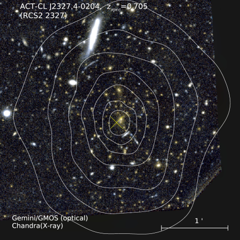
Figure 8.— The Chandra X-ray observation for ACT-CL J2327.4$-$0204, which shows its extended nature, is overlaid as white contours on the $gr$ optical pseudo-color composite image from GMOS. The X-ray contours cover a dynamic range of a factor of 100 from the peak to the minimum.

ACT-CL J2327.4$-$0204 is the cluster with the highest significance detection and the strongest SZ signal in the full ACT equatorial sample. The cluster has also been reported as RCS2 2327 by Gralla et al. (2011). Although the cluster is not in S82, the system is rich and bright enough to be detected on the shallower DR8 imaging from which we obtained an accurate photometric redshift estimate of $z=0.69\pm 0.04$ and optical richness $N_{\rm gal}=59.2\pm 7.7$. We searched for archival data and found imaging and spectroscopy from Gemini/GMOS and X-ray observations from Chandra and XMM-Newton. We processed the single GMOS pointing (offset $2^{\prime}$ from the cluster center) in $g$ ($4\times 300$ s) and $r$ ($4\times 300$ s) taken on UT 2007 Aug 7 and UT 2007 Dec 26 (GS-2007B-Q-5, PI:Gladders) using our GMOS custom pipeline (Sifón et al., 2012) to create astrometrically corrected co-added images. The GMOS imaging of the central region of the cluster, shown in Figure 8, confirms the picture from DR8 that ACT-CL J2327.4$-$0204 is a very rich cluster, and reveals the presence of several strong lensing features. We also processed the spectroscopic data from the single mask available taken with the B600 grism for a total integration time of 14.4 ks of which we were able to process 7.2 ks. Unfortunately the setup of the spectroscopic observations only covers the $4000-6800$Å wavelength range hence putting the CaII K-H absorption doublet (rest-frame $\lambda_{0}=3950$Å) used to secure the redshift of early-type galaxies at the limit of the detector. Nevertheless, we were able to extract redshifts for three cluster galaxies (two of them with [OII] emission), for which we obtain a mean redshift of $z=0.705$.

A 25 ks Chandra observation (PI:Gladders, ObsID 7355) was taken in August of 2008 using the ACIS-S array in VFAINT mode. We processed the data using CIAO version 4.4, applying the latest calibrations (CALDB version 4.5.0). VFAINT background rejection was implemented. X-ray point sources were identified and compared to the locations of their optical counterparts, which established that the absolute astrometry of this Chandra observation was good ($1^{\prime\prime}$). Background was subtracted using the blank-sky background files supplied by the CXC. The process included applying an appropriate filter to the source data to remove time intervals of high background. This observation was devoid of any background flares.

For making images, point sources were removed and replaced with Poisson distributed counts based on the surrounding level of background or source emission. Exposure maps were created in the soft (0.5-2 keV) band. Figure 8 shows surface brightness contours of the background-subtracted, exposure-corrected, adaptively-smoothed Chandra X-ray data in the 0.5–2 keV band. The X-rays show a strongly peaked distribution centered very close to the BCG. The cluster X-ray isophotes are modestly elliptical with an axial ratio of $\sim$1.2 and little centroid shift. We detect X-ray emission out to a mean radius of $\sim 0.\!^{\prime}8$ ($670\,h^{-1}_{70}$ kpc).

We use this observation to measure the gas temperature of the cluster. An absorbed phabs*mekal model yielded a best-fit (source frame) temperature of $kT_{X}=11.0_{-1.3}^{+2.0}$ keV from the core-excised Chandra spectrum (covering from $0.15R_{500c}$ to $0.50R_{500c}$ after iterating to obtain $R_{500c}$). We use this value with Eq. 5 in Vikhlinin et al. (2009) to estimate the cluster temperature within $R_{500c}$ which can then be used in the $T_{X}$-$M_{X}$ scaling law. We also have obtained an integrated spectrum (covering the full cluster out to a radius of $\sim 0.\!^{\prime}8$. From this we obtain a bolometric luminosity of $L_{\rm bol}=(6.6\pm 0.3)\times 10^{45}\,h_{70}^{-2}$ erg s^-1. Figure 9 shows the $L_{\rm bol}$-$T_{X}$ relation with ACT-CL J2327.4$-$0204 added as the red point. The smaller grey points show the sample of Markevitch (1998), while the white square and large grey circle show the closest comparison clusters, 1E0657$-$56 and El Gordo. Similarly, the X-ray luminosity of ACT-CL J2327.4$-$0204 in the 0.5–2.0 keV band is $L_{X}=1.39\pm 0.05\times 10^{45}\,h_{70}^{-2}$erg s^-1.

We follow the prescriptions in Vikhlinin et al. (2009) and apply the $T_{X}-M_{500c}$ scaling law to the Chandra data and obtain a mass of $M_{500c,T_{X}}=9.7^{+3.1}_{-1.8}\times 10^{14}h_{70}^{-1}M_{\odot}$. We also investigated the cluster mass from $M_{\rm gas}$ using the scaling law for $M_{500c}-M_{\rm gas}$ at redshift $z=0.6$ from Kravtsov, Vikhlinin, & Nagai (2006), which yields a value of $M_{500c,\rm Mgas}=(9.6\pm 1.2)\times 10^{14}h_{70}^{-1}M_{\odot}$ and implies a gas mass fraction $f_{\rm gas}=0.12$. Both X-ray derived masses are in good agreement and confirm the view of an exceptional and massive cluster. We use the weighted-average of the $T_{X}$ and $M_{\rm gas}$ mass estimates to obtain a combined mass for ACT-CL J2327.4$-$0204 of $M_{500c}=(1.0\pm 0.1)\times 10^{15}\,h_{70}^{-1}M_{\odot}$. We convert the combined mass with respect to the average density using the same procedure as for ACT-CL J0044.4$+$0113 in Section 4.3.1 using the scaling $M_{200a}=1.86_{-0.20}^{+0.30}\times M_{500c}$ which produces a mass $M_{200a}=1.9_{-0.4}^{+0.6}\times 10^{15}\,h_{70}^{-1}M_{\odot}$. This mass is also consistent with the velocity dispersion of $\approx 1400$ km s^-1 presented by Yee et al. (2009) which indicates a dynamical mass of $M_{200a,\rm dyn}\approx 2.6\times 10^{15}\,h_{70}^{-1}M_{\odot}$ when applying the same procedure as described below (Section 4.3.3). In summary, the high SZ-signal, gas temperature, gas mass and velocity dispersion, taken together, establish ACT-CL J2327.4$-$0204 as one of the two most massive clusters known at $z>0.6$, the other being El Gordo.

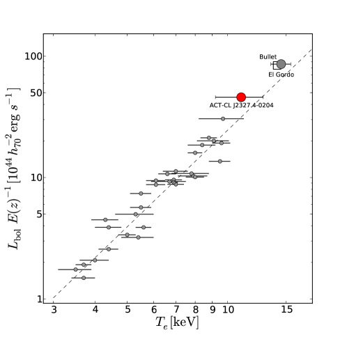
Figure 9.— The X-ray bolometric luminosity vs. temperature for a sample of well-studied clusters taken from Markevitch (1998). The Bullet cluster (1E0657$-$56) and El Gordo are the open square point and gray circle at high temperature and luminosity from Markevitch (2006) and Menanteau et al. (2012) respectively. ACT-CL J2327.4$-$0204 is the red circle that shows the remarkable properties of the cluster. The dashed line represents the $L-T$ best-fit from Markevitch (1998).

4.3.3 ACT-CL J0022.2$-$0036

ACT-CL J0022.2$-$0036 is the highest significance SZ detection on the S82 region of the ACT equatorial sample and has been extensively targeted for our follow-up observations. Reese et al. (2012) recently presented SZA observations of the cluster, while Miyatake et al. (2012) estimated its mass from weak-lensing measurements using Subaru. As part of our spectroscopic follow-up with Gemini (Sifón et al. in prep) we have secured redshifts for 44 members from which we obtain a redshift $z=0.8054\pm 0.0013$ and velocity dispersion of $\sigma_{\rm gal}=1213\pm 155$ km s^-1. We use the $M_{200c}-\sigma_{\rm DM}$ scaling relation from Evrard et al. (2008) to convert the measured velocity dispersion into a dynamical mass estimate,

$$M_{200c}=\frac{10^{15}}{0.7E(z)}\left(\frac{\sigma_{\rm DM}}{\sigma_{{\rm DM},15}}\right)^{1/{\alpha}}\,h_{70}^{-1}\,M_{\odot},$$ (2)

where $\sigma_{{\rm DM},15}=1082.9\pm 4.0$ km s^-1, $\alpha=0.3361\pm 0.0026$ and $\sigma_{\rm DM}$ is the velocity dispersion of the dark matter halo. The latter is related to the observed galaxy velocity dispersion by the velocity bias parameter, $b_{v}=\sigma_{\rm gal}/\sigma_{\rm DM}$. The latest physically motivated simulations (see Evrard et al., 2008, and references therein) indicate that galaxies are essentially unbiased tracers of the dark matter potential, $\langle b_{v}\rangle=1.00\pm 0.05$. Using a bias factor of $b_{v}=1$ for the velocity dispersion for all galaxies, we obtain a dynamical mass of $M_{200a,\rm dyn}=1.5_{-0.6}^{+0.7}\times 10^{15}\,h_{70}^{-1}\,M_{\odot}$, using the conversion factor $M_{200a}=1.17_{-0.03}^{+0.04}M_{200c}$ with the same prescription as described in Section 4.3.1. This value is consistent with the Subaru weak-lensing mass of $M_{200a,{\rm WL}}=1.1^{+0.6}_{-0.5}\times 10^{15}\,h_{70}^{-1}\,M_{\odot}$ recently reported by Miyatake et al. (2012).

5. Discussion

5.1. The Purity of the S82 Sample

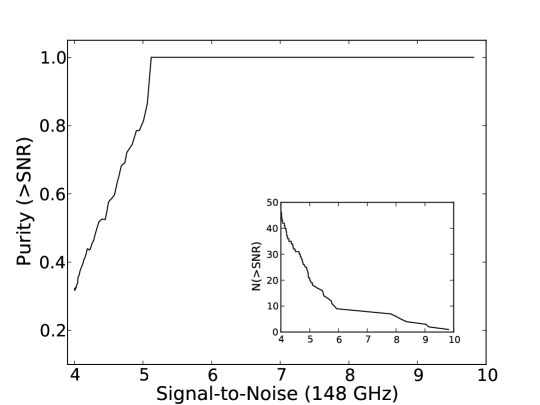
Figure 10.— The S82 SZ cluster sample purity greater than a given S/N in the ACT 148 GHz maps. The purity is defined as the ratio of the number of confirmed clusters to the number of observed clusters candidates. The solid line represents the purity binned in $n=2$ events. The inset plot shows the cluster cumulative distribution as a function of S/N for the optically-confirmed cluster sample.

The purity for an SZ sample is defined as the ratio of optically-confirmed clusters to SZ detections (Menanteau et al., 2010a). In Figure 10 we show the purity from the sample of 155 SZ cluster candidates with S/N$>4.0$ within the S82 region as a function of signal-to-noise. A notable improvement from our previous work on the southern sample (Menanteau et al., 2010a) is that for the S82 region we were able to examine every cluster candidate regardless of its signal-to-noise. The inset plot shows the cluster cumulative distribution as a function of S/N for the optically-confirmed cluster sample. We achieve 100% purity for signal-to-noise ratios greater than 5.1 where there are 19 clusters. This drops to a purity value of 80% for a SNR of 5.0. For SZ candidates down to a signal-to-noise of 4.6 the sample the purity is 60% (31/52). Below this S/N value we find a purity value of only 30% down to a signal-to-noise of 4.0. It is important to mention that we did not perform targeted follow-up in the NIR for all SZ candidates without a clear optical identification. We obtained $K_{S}$ for all of candidates above S/N$>5.1$, but only for a fraction of those above S/N$>4.7$. Therefore some of the clusters that were not optically confirmed could potentially be at $z>1$. The purity of the S82 sample is consistent with the purity we found for the ACT southern sample.

5.2. Cluster X-ray Properties

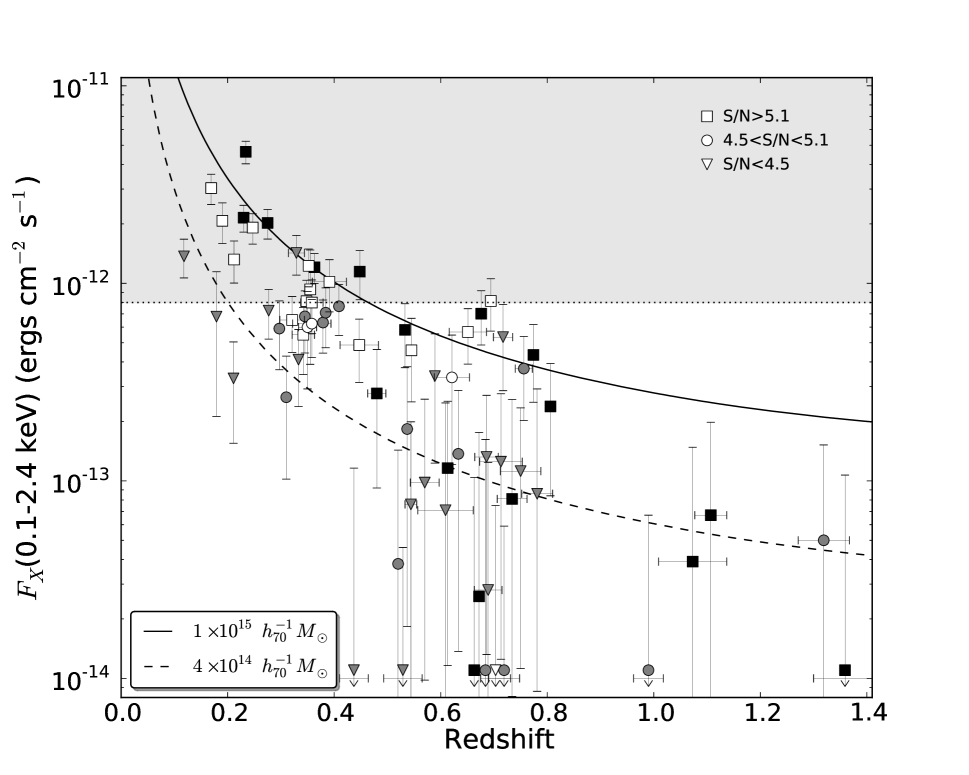
Figure 11.— The soft X-ray flux (in the observed band of 0.1–2.4 keV) from RASS archival data as a function of redshift for ACT SZ equatorial clusters. Clusters with S/N$>5.1$, are shown as boxes, circles represent clusters with $4.5<$S/N$<5.1$ and triangles clusters S/N$<4.5$. White filled symbols represent objects outside the S82 the deep region. For non detection sources we show upper limits. The dashed and solid curves represent the expected X-ray fluxes for clusters with masses $M_{200a}=4\times 10^{14}\,h_{70}^{-1}M_{\odot}$ and $1\times 10^{15}\,h_{70}^{-1}M_{\odot}$, respectively, using scaling relations from Vikhlinin et al. (2009). The gray area at the top corresponds approximately to the regime of the RASS bright source catalog (Voges et al., 1999).

For consistency with our previous work (Menanteau et al., 2010a) and to establish qualitatively that the ACT clusters indeed comprise a massive sample, we present the RASS X-ray fluxes and luminosities for all confirmed ACT clusters, regardless of the significance of the RASS detection in Tables 4 and 5. The soft RASS X-ray fluxes as a function of redshift are plotted in Figure 11. We indicate the region at the high-end flux that approximately corresponds to the flux limit of the RASS bright source catalog (Voges et al., 1999). In cases of no significant detection we indicate upper limits. Clusters detected with higher significance (S/N$>4.5$) in the ACT 148 GHz data are shown as black squares while the others are represented by gray circles. The low statistical quality of the RASS data for most of these clusters precludes making accurate estimates of cluster masses from the X-ray data. However, for reference we show curves of the expected (observed-frame) X-ray fluxes for clusters with assumed masses of $M_{200a}=4\times 10^{14}h_{70}^{-1}M_{\odot}$ (dashed) and $1\times 10^{15}h_{70}^{-1}M_{\odot}$ (solid) using the X-ray luminosity versus mass scaling relation in Vikhlinin et al. (2009). We use their Eq. 22, which includes an empirically determined redshift evolution. We convert their X-ray band (emitted: 0.5–2 keV band) to ours (observed: 0.1–2.4 keV) assuming a thermal spectrum at the estimated cluster temperature determined using the mass-temperature relation also from Vikhlinin et al. (2009). This too has a redshift dependence, so the estimated temperatures vary in the ranges 2.9–5.0 keV and 5.2–9.0 keV over $0.0<z<1.1$ for the two mass values we plot (solid and dashed lines). We use conversion factors assuming the redshift-averaged temperatures of 4 keV and 7 keV, since the difference in conversion factor over the temperature ranges is only a few percent, negligible on the scale of Figure 11. The mass values in Vikhlinin et al. (2009) are defined with respect to an overdensity of 500 times the critical density of the Universe at the cluster redshift. As we have done before, we convert to an overdensity of 200 times the average density following the procedure in Section 4.3.1. This mass conversion factor is approximately 1.8 averaged over redshift, varies from 2.2 to 1.7 over $0.0<z<1.1$, and depends only weakly on cluster mass (few percent) for the 2 values plotted here.

The X-ray fluxes for the ACT SZ-selected clusters scatter around the $4\times 10^{14}\,h_{70}^{-1}M_{\odot}$ and $1\times 10^{15}\,h_{70}^{-1}M_{\odot}$ curves, for the full and pure samples respectively, validating that this is a massive cluster sample.

5.3. Mass Estimation

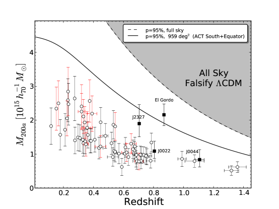
Figure 12.— The exclusion curves, $M_{200a}(z)$, from the Mortonson, Hu, & Huterer (2011) fitting formulas where a single cluster above the corresponding curve would conflict with Flat $\Lambda$CDM and quintessence at 95% C.L for both sample and parameters variance. The dashed and solid lines represent the exclusion curves for the full sky and the ACT survey analyzed region of 959 deg² (i.e. the mass limit for a cluster at a given redshift that it is less than 5% likely to be found in 95% of the $\Lambda$CDM parameter probability distribution). The open circles with black and red error bars represent the $M_{200a}$ mass estimates using the $\widetilde{y}_{0}-M$ scaling law (Sifón et al., 2012) for clusters inside and outside of S82 respectively. We also show the X-ray mass estimates based for ACT-CL J0044.4$+$0113 and ACT-CL J2327.4$-$0204 (combined) as black squares. For ACT-CL J0022.2$-$0036 we show its dynamical mass from the Gemini observations. For reference, we also show our combined mass estimate for El Gordo, with 1-$\sigma$ error bars (Menanteau et al., 2012).

In order to obtain consistent estimates across the full ACT equatorial sample we use the $\widetilde{y}_{0}-M_{200c}$ scaling relation from Sifón et al. (2012), which relates the fixed aperture central Compton decrement $\widetilde{y}_{0}$ as described by Hasselfield et al. (2013) and $M_{200c}$ (critical) for the cluster as

$$M_{200c}=10^{(15.03\pm 0.07)}\,\left(\frac{\widetilde{y}_{0}E(z)^{-2}}{5\times 10^{-5}}\right)^{0.74\pm 0.11}h_{70}^{-1}M_{\odot}.$$ (3)

We use the $\widetilde{y}_{0}$ measurements from Table 3 from Hasselfield et al. (2013) to estimate $M_{200c}$ for the sample which in turn we transform to $M_{200a}$ (average) using the same procedure described in Section 4.3.1. For a comparison with the dynamical masses from Sifón et al. (2012) and the effects of different models of gas pressure profile in cluster SZ mass see Hasselfield et al. (2013).

In Figure 12 we show the SZ-derived masses for the whole sample as a function of their redshift using the above mass-scaling relation. We also compare the masses of the cluster sample with the $M_{200a}(z)$ exclusion curves from Mortonson, Hu, & Huterer (2011) for which a single cluster with mass $M_{200a}$ above the corresponding curve would conflict with $\Lambda$CDM and quintessence at 95% confidence level, including both sample and cosmological parameter variance. In other words, the exclusion curves represent the mass threshold as a function of redshift for which any cluster is less than 5% likely to be found in a survey region for 95% of the $\Lambda$CDM parameter variance. In order to address the rarity of any of our clusters in Fig. 12 we plot the exclusion curves for the full sky and the region analyzed for the ACT survey (959 deg²). We note, however, that Harrison & Hotchkiss (2012) have recently suggested that these curves tend to overestimate the amount of tension with cosmological models because they underestimate the number of massive clusters due to an inadequate a posteriori choice of mass and redshift cuts. In the figure, we show the X-ray mass estimates for ACT-CL J0044.4$+$0113 and ACT-CL J2327.4$-$0204 (combined), plus the dynamical mass of ACT$-$CL J0022.2$-$0036 and El Gordo (for comparison), as black squares.

5.4. Distance between SZ Centroid and BCG

An important source of systematic uncertainty in studies of large optically-selected clusters is the “miscentering” of the BCG with respect to the dark matter (DM) and hot gas. This may be the result from either a misidentification of the BCG by the finding algorithm, or a real physical offset between the DM and gas centers and the BCG. The latter can be a real astrophysical observable linked to the cluster dynamical state, while the former is essentially just a flaw in the identification algorithm (see Skibba et al., 2011; George et al., 2012, for examples of recent studies).

Prompted by the results from Planck Collaboration et al. (2011b) where the predicted $Y_{SZ}$ from the $Y_{SZ}-N_{200}$ relation (Rozo et al., 2009) was much higher than the observed stacked $Y_{SZ}$ signal for the MaxBCG clusters (Koester et al., 2007), some studies have considered miscentering to explain this discrepancy (e.g. Biesiadzinski et al., 2012; Sehgal et al., 2012), while others favor solutions that include uncertainties in optical systematics and selection effects (Angulo et al., 2012; Rozo, et al., 2012). Our sample of SZ galaxy clusters allows us to directly investigate the offsets between the SZ centroid position in the 148 GHz ACT maps and the location of the BCG on the optical images. One key advantage of our sample is that the BCG identification has been performed visually in all cases to ensure that it is indeed the brightest member in the cluster and hence is virtually free of bias due to miscentering. We compute the offsets between the BCG and SZ centroid position for the high-significance sample (S/N$>5.1$) and the full sample (Figure 13) for the S82 region. We find that the typical distance to the BCG is less than $0.3$ Mpc $h_{70}^{-1}$ for both samples, with mean distance values of $0.12$ Mpc $h_{70}^{-1}$ and $0.17$ Mpc $h_{70}^{-1}$ for the high-significance and the full sample respectively. We therefore find no significant evidence for the amount of misalignment required to explain the discrepancy between $Y_{SZ}$ and $N_{200}$ by Planck to be a physical offset, as opposed to algorithmic, between the BCG and the gas center. We note that the typical positional uncertainty of the ACT SZ centroid for cluster is $\approx 1^{\prime}.4/$ SNR which for S/N$=4.5$ corresponds to $0.12\,h_{70}^{-1}$ Mpc and $0.16\,h_{70}^{-1}$ Mpc at $z=0.5$ and $z=1.0$ respectively. Thus the observed level of offset can be accounted by the uncertainty in the ACT cluster centering.

Figure 13.— The distribution of the distances in co-moving units between the ACT centroid SZ position and the location of the BCG in the optical images for the high-significance sample (right panel, S/N$>5.1$) and the full sample (left panel, S/N$>4$).

5.5. SZ-Optical Richness Relation

The continuous optical coverage provided by SDSS over S82 and DR8 for our cluster sample also enables a direct and independent investigation of the relation between optical richness and SZ signal. For this purpose, we use our own computed $N_{200}$ values for clusters as described in Section 3.3 and compare with their SZ-derived $M_{200a}$ masses (using the same values as above in Section 4.3). We only consider clusters at $z<0.65$ within S82 and $z<0.40$ outside S82 to take into account the different flux limits of the two samples to ensure unbiased values of $N_{200}$ and hence allow for a meaningful comparison. In Figure 14 we show the results with symbols keyed to the location of the clusters (inside or outside S82) color-keyed to their redshifts. A simple examination of the individual points hints of a weak correlation with high scatter between the optical richness with SZ mass. For this data set we calculate a Pearson’s correlation coefficient of $r=0.52$ and probability of an uncorrelated system producing a correlation at least as extreme as the one computed of $p=0.0004$ which indicates a real correlation but with significant scatter. In order to bring visual clarity in the scatter we estimate the mean-weighted SZ mass as a function of $N_{200}$ in bins of size $\Delta N_{200}=30$ which we also show in Figure 14. The errors were estimated as the quadratic sum of the weighted errors and the error in the mean. We conclude that optical richness estimates such as $N_{200}$ for modest-sized samples like this one do not provide precise mass estimates.

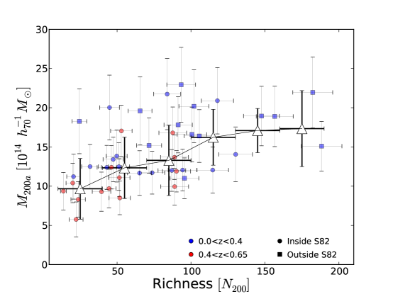
Figure 14.— The SZ-derived $M_{200a}$ mass from using Sifón et al. (2012) $\widetilde{y_{0}}-M$ scaling relation for SZ equatorial clusters compared to their optical richness $N_{200}$. We show clusters on S82 as circles and systems outside that area as squares. Additionally, we colored red the systems located at $z>0.4$ and blue at $z<0.4$. Open triangles denote the weighted mean mass value in bins of size $\Delta N_{200}=30$.

6. Summary and Conclusions

We present the optical/NIR confirmation and physical properties of a new sample of 68 SZ detected clusters from ACT over the celestial equator. Our study takes advantage of the wide and deep coverage over S82 which with additional pointed NIR observations enabled the characterization of 49 clusters up to $z\approx 1.3$. Although this is a well-studied region of the sky, 22 of the 49 clusters on the S82 region are newly discovered systems all lying at $z>0.55$, highlighting the power of the SZ effect to discover massive clusters at high redshift. Moreover, five of these clusters are at $z\geq 1$. Outside the S82 region we use the regular-depth SDSS data from DR8 to confirm 19 additional clusters to $z\approx 0.7$, with 10 systems discovered by ACT. We have also analysed ROSAT All-Sky Survey data for the sample, which confirms that this is a high-mass cluster sample.

The S82 optical data provides a powerful complement as it allows the study of every SZ cluster candidate down to any ACT S/N desired. Preliminary inspection of lower S/N candidates finds several rich optical systems, suggesting that improved multi-wavelength cluster-finding algorithms may allow for additional discoveries.

We investigate differences in the location of the BCG and the SZ centroid positions and we find no evidence for significant offsets between them. We also study the relation between the optical richness and cluster mass and find only a weak correlation between both quantities.

As with the ACT southern sample, we find some spectacular systems in the ACT equatorial sample. We report on the discovery of ACT-CL J0044.4$+$0113, at $z=1.1$, with mass and X-ray temperature that put it in the league of the extreme clusters at $z>1$. We also present a multi-wavelength analysis of the rich cluster ACT-CL J2327.4$-$0204 at $z=0.705$. This is the cluster with the highest SZ significance in the whole ACT equatorial sample and is comparable to systems like El Gordo and the Bullet Cluster.

Based on currently available mass estimates there is no tension between $\Lambda$CDM and the sample’s mass-redshift distribution. El Gordo and ACT-CL J2327.4$-$0204 are the most extreme clusters in the joint ACT sample, and more detailed, multi-wavelength follow-up studies will aid in further constraining the masses and physical properties of these clusters, as well as their cosmological implications.

Table 4ROSAT Properties of Stripe 82 ACT equatorial cluster

		$t_{\rm exp}$	$N_{H}$	$R$	$F_{X}$	$L_{X}$
ACT Descriptor	$z$	(s)	($10^{20}$ cm-2)	($h_{70}^{-1}$ kpc)	(0.1$-$2.4 keV)	(0.1$-$2.4 keV)
ACT-CL J0012.0$-$0046	1.36	369	3.22	1514	$0.01\pm 0.97$	$0.11\pm 7.59$
ACT-CL J0014.9$-$0057	0.533	357	3.06	1136	$5.81\pm 2.07$	$5.30\pm 1.89$
ACT-CL J0017.6$-$0051	0.211	351	2.93	619	$3.30\pm 1.75$	$0.39\pm 0.21$
ACT-CL J0018.2$-$0022	0.75	372	2.69	1321	$1.12\pm 1.22$	$2.23\pm 2.43$
ACT-CL J0022.2$-$0036	0.806	398	2.76	1355	$2.38\pm 1.54$	$5.59\pm 3.61$
ACT-CL J0044.4$+$0113	1.11	304	1.86	1473	$0.67\pm 1.31$	$3.29\pm 6.39$
ACT-CL J0051.1$+$0055	0.69	365	2.41	1278	$0.28\pm 0.96$	$0.46\pm 1.58$
ACT-CL J0058.0$+$0030	0.76	384	2.82	1324	$3.70\pm 1.68$	$7.50\pm 3.40$
ACT-CL J0059.1$-$0049	0.77	356	3.33	1336	$4.34\pm 1.84$	$9.29\pm 3.92$
ACT-CL J0104.8$+$0002	0.277	428	3.31	758	$7.27\pm 2.05$	$1.54\pm 0.43$
ACT-CL J0119.9$+$0055	0.72	425	3.12	1300	$<0.49$	$<0.89$
ACT-CL J0127.2$+$0020	0.379	431	2.90	935	$6.33\pm 1.90$	$2.69\pm 0.81$
ACT-CL J0152.7$+$0100	0.230	432	2.75	661	$21.49\pm 3.33$	$3.04\pm 0.47$
ACT-CL J0206.2$-$0114	0.68	388	2.53	1268	$7.02\pm 2.15$	$11.01\pm 3.37$
ACT-CL J0215.4$+$0030	0.73	164	2.83	1310	$0.81\pm 1.77$	$1.53\pm 3.34$
ACT-CL J0218.2$-$0041	0.672	194	2.96	1265	$0.26\pm 1.50$	$0.40\pm 2.32$
ACT-CL J0219.8$+$0022	0.537	182	2.88	1140	$1.83\pm 1.95$	$1.70\pm 1.81$
ACT-CL J0221.5$-$0012	0.589	211	2.75	1193	$3.39\pm 2.16$	$3.88\pm 2.48$
ACT-CL J0223.1$-$0056	0.663	220	2.94	1258	$<0.94$	$<1.41$
ACT-CL J0228.5$+$0030	0.72	229	2.28	1298	$5.34\pm 2.48$	$9.58\pm 4.46$
ACT-CL J0230.9$-$0024	0.44	190	2.07	1019	$<1.06$	$<0.62$
ACT-CL J0241.2$-$0018	0.684	192	2.95	1274	$<1.52$	$<2.44$
ACT-CL J0245.8$-$0042	0.179	89	3.43	544	$6.78\pm 4.66$	$0.56\pm 0.38$
ACT-CL J0250.1$+$0008	0.78	183	5.09	1340	$0.86\pm 2.06$	$1.88\pm 4.49$
ACT-CL J0256.5$+$0006	0.363	689	6.16	910	$12.06\pm 2.07$	$4.65\pm 0.80$
ACT-CL J0301.1$-$0110	0.53	1281	6.92	1131	$<0.36$	$<0.32$
ACT-CL J0308.1$+$0103	0.633	295	5.93	1233	$1.37\pm 1.50$	$1.85\pm 2.03$
ACT-CL J0320.4$+$0032	0.384	351	6.31	943	$7.10\pm 2.38$	$3.10\pm 1.04$
ACT-CL J0326.8$-$0043	0.448	300	6.76	1034	$11.46\pm 3.20$	$7.07\pm 1.97$
ACT-CL J0336.9$-$0110	1.32	511	7.61	1510	$0.50\pm 1.02$	$3.61\pm 7.40$
ACT-CL J0342.0$+$0105	1.07	365	7.44	1464	$0.39\pm 1.09$	$1.79\pm 4.96$
ACT-CL J0342.7$-$0017	0.310	385	6.04	820	$2.65\pm 1.63$	$0.72\pm 0.44$
ACT-CL J0348.6$-$0028	0.345	357	9.87	881	$6.80\pm 2.36$	$2.34\pm 0.81$
ACT-CL J0348.6$+$0029	0.297	344	9.96	796	$5.90\pm 2.25$	$1.46\pm 0.56$
ACT-CL J2050.5$-$0055	0.613	432	6.24	1215	$1.16\pm 1.37$	$1.46\pm 1.72$
ACT-CL J2051.1$+$0056	0.333	460	7.44	860	$4.11\pm 1.73$	$1.31\pm 0.55$
ACT-CL J2055.4$+$0105	0.409	456	7.54	980	$7.65\pm 2.20$	$3.85\pm 1.11$
ACT-CL J2129.6$+$0005	0.234	275	3.63	670	$46.33\pm 6.05$	$6.81\pm 0.89$
ACT-CL J2130.1$+$0045	0.71	277	3.71	1295	$1.25\pm 1.51$	$2.22\pm 2.68$
ACT-CL J2135.1$-$0102	0.33	323	3.87	853	$14.24\pm 3.24$	$4.42\pm 1.01$
ACT-CL J2135.7$+$0009	0.118	362	4.27	384	$13.69\pm 3.04$	$0.47\pm 0.10$
ACT-CL J2152.9$-$0114	0.69	331	7.46	1276	$1.32\pm 1.39$	$2.14\pm 2.26$
ACT-CL J2154.5$-$0049	0.48	352	7.42	1075	$2.77\pm 1.85$	$2.00\pm 1.33$
ACT-CL J2220.7$-$0042	0.57	231	4.74	1174	$0.98\pm 1.61$	$1.04\pm 1.72$
ACT-CL J2229.2$-$0004	0.61	243	4.73	1211	$0.71\pm 1.77$	$0.88\pm 2.19$
ACT-CL J2253.3$-$0031	0.54	356	5.43	1148	$0.76\pm 1.23$	$0.73\pm 1.18$
ACT-CL J2302.5$+$0002	0.520	348	4.02	1121	$0.38\pm 1.05$	$0.32\pm 0.91$
ACT-CL J2337.6$+$0016	0.275	379	3.55	754	$20.21\pm 3.46$	$4.23\pm 0.72$
ACT-CL J2351.7$+$0009	0.99	376	3.48	1438	$<0.57$	$<2.13$

Table 5ROSAT Properties of ACT equatorial cluster outside Stripe 82

		$t_{\rm exp}$	$N_{H}$	$R$	$F_{X}$	$L_{X}$
ACT Descriptor	$z$	(s)	($10^{20}$ cm-2)	($h_{70}^{-1}$ kpc)	(0.1$-$2.4 keV)	(0.1$-$2.4 keV)
ACT-CL J0008.1$+$0201	0.36	386	2.72	902	$6.25\pm 2.04$	$2.34\pm 0.76$
ACT-CL J0026.2$+$0120	0.65	504	2.86	1248	$5.67\pm 1.77$	$8.16\pm 2.54$
ACT-CL J0045.2$-$0152	0.545	311	2.81	1149	$4.58\pm 2.07$	$4.40\pm 1.99$
ACT-CL J0139.3$-$0128	0.70	320	2.89	1288	$<0.65$	$<1.11$
ACT-CL J0156.4$-$0123	0.45	424	2.56	1033	$4.87\pm 1.72$	$2.99\pm 1.06$
ACT-CL J0219.9$+$0129	0.35	164	3.31	889	$6.00\pm 3.08$	$2.13\pm 1.09$
ACT-CL J0239.8$-$0134	0.375	84	3.01	897	$9.32\pm 5.43$	$3.42\pm 1.99$
ACT-CL J0240.0$+$0116	0.62	235	2.92	1222	$3.34\pm 2.13$	$4.32\pm 2.75$
ACT-CL J0301.6$+$0155	0.167	214	6.57	570	$20.72\pm 4.82$	$1.94\pm 0.45$
ACT-CL J0303.3$+$0155	0.153	254	6.61	519	$30.35\pm 5.30$	$2.21\pm 0.39$
ACT-CL J2025.2$+$0030	0.34	444	9.53	876	$5.49\pm 2.04$	$1.85\pm 0.69$
ACT-CL J2050.7$+$0123	0.333	461	7.71	886	$8.12\pm 2.24$	$2.85\pm 0.79$
ACT-CL J2051.1$+$0215	0.321	462	7.87	892	$12.26\pm 2.66$	$4.42\pm 0.96$
ACT-CL J2058.8$+$0123	0.32	454	6.73	840	$6.52\pm 2.05$	$1.91\pm 0.60$
ACT-CL J2128.4$+$0135	0.39	281	4.07	954	$10.17\pm 3.00$	$4.63\pm 1.36$
ACT-CL J2135.2$+$0125	0.231	398	4.25	697	$19.15\pm 3.36$	$3.17\pm 0.56$
ACT-CL J2156.1$+$0123	0.224	317	4.79	621	$13.20\pm 3.17$	$1.57\pm 0.38$
ACT-CL J2307.6$+$0130	0.36	341	4.31	902	$7.99\pm 2.41$	$2.99\pm 0.90$
ACT-CL J2327.4$-$0204	0.705	367	4.74	1282	$8.14\pm 2.41$	$13.56\pm 4.02$

References

- Abazajian et al. (2009) Abazajian, K. N., et al. 2009, ApJS, 182, 543
- Abell (1958) Abell, G. O. 1958, ApJS, 3, 211
- Aihara et al. (2011) Aihara, H., et al. 2011, ApJS, 193, 29
- Allen, Evrard, & Mantz (2011) Allen, S. W., Evrard, A. E., & Mantz, A. B. 2011, ARA&A, 49, 409
- Angulo et al. (2012) Angulo, R. E., Springel, V., White, S. D. M., Jenkins, A., Baugh, C. M., & Frenk, C. S. 2012, arXiv:1203.3216
- Annis et al. (2011) Annis, J., et al. 2011, arXiv:1111.6619
- Arnaud, Pointecouteau, & Pratt (2005) Arnaud, M., Pointecouteau, E., & Pratt, G. W. 2005, A&A, 441, 893
- Arnaud et al. (2010) Arnaud, M., Pratt, G. W., Piffaretti, R., Böhringer, H., Croston, J. H., & Pointecouteau, E. 2010, A&A, 517, A92
- Auger et al. (2009) Auger, M. W., Treu, T., Bolton, A. S., Gavazzi, R., Koopmans, L. V. E., Marshall, P. J., Bundy, K., & Moustakas, L. A. 2009, ApJ, 705, 1099
- Benítez (2000) Benítez, N. 2000, ApJ, 536, 571
- Benítez et al. (2004) Benítez, N., et al. 2004, ApJS, 150, 1
- Bertin & Arnouts (1996) Bertin, E., & Arnouts, S. 1996, A&AS, 117, 393
- Bertin et al. (2002) Bertin, E., Mellier, Y., Radovich, M., Missonnier, G., Didelon, P., & Morin, B. 2002, Astronomical Data Analysis Software and Systems XI, 281, 228
- Bertin (2006) Bertin, E. 2006, Astronomical Data Analysis Software and Systems XV, 351, 112
- Biesiadzinski et al. (2012) Biesiadzinski, T., McMahon, J. J., Miller, C. J., Nord, B., & Shaw, L. 2012, arXiv:1201.1282
- Birkinshaw (1999) Birkinshaw, M. 1999, Phys. Rep., 310, 97
- Blanton et al. (2003) Blanton, M. R., et al. 2003, ApJ, 592, 819
- Böhringer et al. (2000) Böhringer, H., et al. 2000, ApJS, 129, 435
- Bruzual & Charlot (2003) Bruzual, G., & Charlot, S. 2003, MNRAS, 344, 1000
- Carlstrom, Holder, & Reese (2002) Carlstrom, J. E., Holder, G. P., & Reese, E. D. 2002, ARA&A, 40, 643
- Coleman et al. (1980) Coleman, G. D., Wu, C.-C., & Weedman, D. W. 1980, ApJS, 43, 393
- Das et al. (2011a) Das, S., et al. 2011a, ApJ, 729, 62
- Das et al. (2011b) Das, S., et al. 2011b, Physical Review Letters, 107, 021301
- Duffy et al. (2008) Duffy, A. R., Schaye, J., Kay, S. T., & Dalla Vecchia, C. 2008, MNRAS, 390, L64
- Dunkley et al. (2011) Dunkley, J., et al. 2011, ApJ, 739, 52
- Dünner et al. (2012) Dünner, R., et al. 2012, arXiv:1208.0050
- Evrard et al. (2008) Evrard, A. E., et al. 2008, ApJ, 672, 122
- Foley et al. (2011) Foley, R. J., et al. 2011, ApJ, 731, 86
- Fowler & Gatley (1990) Fowler, A. M., & Gatley, I. 1990, ApJ, 353, L33
- Fowler et al. (2007) Fowler, J. W., et al. 2007, Appl. Opt., 46, 3444
- Geach, Murphy, & Bower (2011) Geach, J. E., Murphy, D. N. A., & Bower, R. G. 2011, MNRAS, 413, 3059
- George et al. (2012) George, M. R., et al. 2012, ApJ, 757, 2
- Gralla et al. (2011) Gralla, M. B., et al. 2011, ApJ, 737, 74
- Hajian et al. (2011) Hajian, A., et al. 2011, ApJ, 740, 86
- Hand et al. (2011) Hand, N., et al. 2011, ApJ, 736, 39
- Hand et al. (2012) Hand, N., et al. 2012, Physical Review Letters, 109, 041101
- Hansen et al. (2005) Hansen, S. M., McKay, T. A., Wechsler, R. H., Annis, J., Sheldon, E. S., & Kimball, A. 2005, ApJ, 633, 122
- Hao et al. (2010) Hao, J., et al. 2010, ApJS, 191, 254
- Harrison & Hotchkiss (2012) Harrison, I., & Hotchkiss, S. 2012, arXiv:1210.4369
- Hasselfield et al. (2013) Hasselfield, M., et al. 2013, arXiv:1301.0816
- High et al. (2010) High, F. W., et al. 2010, ApJ, 723, 1736
- Hicken et al. (2009) Hicken, M., Wood-Vasey, W. M., Blondin, S., Challis, P., Jha, S., Kelly, P. L., Rest, A., & Kirshner, R. P. 2009, ApJ, 700, 1097
- Hincks et al. (2010) Hincks, A. D., et al. 2010, ApJS, 191, 423
- Hlozek et al. (2012) Hlozek, R., et al. 2012, ApJ, 749, 90
- Hoyle, Jimenez, & Verde (2011) Hoyle, B., Jimenez, R., & Verde, L. 2011, Phys. Rev. D, 83, 103502
- Jee et al. (2009) Jee, M. J., et al. 2009, ApJ, 704, 672
- Kalberla et al. (2005) Kalberla, P. M. W., Burton, W. B., Hartmann, Dap, Arnal, E. M., Bajaja, E., Morras, R., & Pöppel, W. G. L. 2005, A&A, 440, 775
- Kinney et al. (1996) Kinney, A. L., Calzetti, D., Bohlin, R. C., McQuade, K., Storchi-Bergmann, T., & Schmitt, H. R. 1996, ApJ, 467, 38
- Koester et al. (2007) Koester, B. P., et al. 2007, ApJ, 660, 239
- Komatsu et al. (2011) Komatsu, E., et al. 2011, ApJS, 192, 18
- Kravtsov, Vikhlinin, & Nagai (2006) Kravtsov, A. V., Vikhlinin, A., & Nagai, D. 2006, ApJ, 650, 128
- Lawrence et al. (2007) Lawrence, A., et al. 2007, MNRAS, 379, 1599
- Markevitch (1998) Markevitch, M. 1998, ApJ, 504, 27
- Markevitch (2006) Markevitch, M. 2006, The X-ray Universe 2005, 604, 723
- Marriage et al. (2011a) Marriage, T. A., et al. 2011, ApJ, 737, 61
- Marriage et al. (2011b) Marriage, T. A., et al. 2011, ApJ, 731, 100
- Menanteau et al. (2009) Menanteau, F., et al. 2009, ApJ, 698, 1221
- Menanteau & Hughes (2009) Menanteau, F., & Hughes, J. P. 2009, ApJ, 694, L136
- Menanteau et al. (2010a) Menanteau, F., et al. 2010a, ApJ, 723, 1523
- Menanteau et al. (2010b) Menanteau, F., et al. 2010b, ApJS, 191, 340
- Menanteau et al. (2012) Menanteau, F., et al. 2012, ApJ, 748, 7
- Miyatake et al. (2012) Miyatake, H., et al. 2012, arXiv:1209.4643
- Mortonson, Hu, & Huterer (2011) Mortonson, M. J., Hu, W., & Huterer, D. 2011, Phys. Rev. D, 83, 023015
- Nagai, Kravtsov, & Vikhlinin (2007) Nagai, D., Kravtsov, A. V., & Vikhlinin, A. 2007, ApJ, 668, 1
- Navarro, Frenk, & White (1997) Navarro, J. F., Frenk, C. S., & White, S. D. M. 1997, ApJ, 490, 493
- Percival et al. (2010) Percival, W. J., et al. 2010, MNRAS, 401, 2148
- Planck Collaboration et al. (2011a) Planck Collaboration, et al. 2011a, A&A, 536, A8
- Planck Collaboration et al. (2011b) Planck Collaboration, et al. 2011b, A&A, 536, A12
- Reichardt et al. (2012) Reichardt, C. L., et al. 2012, arXiv:1203.5775
- Reese et al. (2012) Reese, E. D., et al. 2012, ApJ, 751, 12
- Rosati et al. (2009) Rosati, P., et al. 2009, A&A, 508, 583
- Rozo et al. (2009) Rozo, E., et al. 2009, ApJ, 703, 601
- Rozo et al. (2010) Rozo, E., et al. 2010, ApJ, 708, 645
- Rozo, et al. (2012) Rozo, E., Bartlett, J. G., Evrard, A. E., & Rykoff, E. S. 2012, arXiv:1204.6305
- Sarazin, Rood, & Struble (1982) Sarazin, C. L., Rood, H. J., & Struble, M. F. 1982, A&A, 108, L7
- Sifón et al. (2012) Sifón, C., et al. 2012, arXiv:1201.0991
- Sehgal et al. (2011) Sehgal, N., et al. 2011, ApJ, 732, 44
- Sehgal et al. (2012) Sehgal, N., et al. 2012, arXiv:1205.2369
- Sherwin et al. (2012) Sherwin, B. D., Das, S., Hajian, A., et al. 2012, arXiv:1207.4543
- Skibba et al. (2011) Skibba, R. A., van den Bosch, F. C., Yang, X., More, S., Mo, H., & Fontanot, F. 2011, MNRAS, 410, 417
- Skrutskie et al. (2006) Skrutskie, M. F., et al. 2006, AJ, 131, 1163
- Staniszewski et al. (2009) Staniszewski, Z., et al. 2009, ApJ, 701, 32
- Stalder et al. (2012) Stalder, B., et al. 2012, arXiv:1205.6478
- Struble & Rood (1991) Struble, M. F., & Rood, H. J. 1991, ApJS, 77, 363
- Sullivan et al. (2011) Sullivan, M., et al. 2011, ApJ, 737, 102
- Sunyaev & Zeldovich (1972) Sunyaev, R. A., & Zeldovich, Y. B. 1972, Comments on Astrophysics and Space Physics, 4, 173
- Suzuki et al. (2012) Suzuki, N., et al. 2012, ApJ, 746, 85
- Swetz et al. (2011) Swetz, D. S., et al. 2011, ApJS, 194, 41
- Tinker et al. (2008) Tinker, J., Kravtsov, A. V., Klypin, A., Abazajian, K., Warren, M., Yepes, G., Gottlöber, S., & Holz, D. E. 2008, ApJ, 688, 709
- Voges et al. (1999) Voges, W., et al. 1999, A&A, 349, 389
- Vikhlinin et al. (2009) Vikhlinin, A., et al. 2009, ApJ, 692, 1060
- Vanderlinde et al. (2010) Vanderlinde, K., et al. 2010, ApJ, 722, 1180
- Waizmann, Ettori, & Moscardini (2012) Waizmann, J.-C., Ettori, S., & Moscardini, L. 2012, MNRAS, 420, 1754
- Wen, Han, & Liu (2009) Wen, Z. L., Han, J. L., & Liu, F. S. 2009, ApJS, 183, 197
- Williamson et al. (2011) Williamson, R., et al. 2011, ApJ, 738, 139
- Yee et al. (2009) Yee, H., et al. 2009, Presented in the conference Galaxy Evolution and Environment, Kuala Lumpur, Malaysia, 30 March - 3 April, 2009.
- Zwicky, Herzog, & Wild (1963) Zwicky, F., Herzog, E., & Wild, P. 1963, Pasadena: California Institute of Technology (CIT), c1963,