Inflationary Dynamics with a Non-Abelian Gauge Field

Abstract

We study the dynamics of the universe with a scalar field and an SU(2) non-Abelian Gauge (Yang-Mills) field. The scalar field has an exponential potential and the Yang-Mills field is coupled to the scalar field with an exponential function of the scalar field. We find that the magnetic component of the Yang-Mills field assists acceleration of the cosmic expansion and a power-law inflation becomes possible even if the scalar field potential is steep, which may be expected from some compactification of higher-dimensional unified theories of fundamental interactions. This power-law inflationary solution is a stable attractor in a certain range of coupling parameters. Unlike the case with multiple Abelian gauge fields, the power-law inflationary solution with the dominant electric component is unstable because of the existence of non-linear coupling of the Yang-Mills field. We also analyze the dynamics for the non-inflationary regime, and find several attractor solutions.

I Introduction

The idea of inflation now gives a standard scenario of the early evolution of the universe Starobinsky ; inflation1 ; inflation2 ; inflation3 ; inflation4 . It solves several difficulties such as the horizon and flatness problems in the Big-Bang cosmology, which has been confirmed by the precision cosmological observations. It also provides us with a prediction on the origin of the observed density fluctuations. Many cosmological models with such a phase of accelerated expansion have been proposed by introducing a scalar field with an appropriate potential (or some alternative fields). However, it is desirable to derive a natural model from a fundamental theory of particle physics without introducing any anonymous field by hand. The most promising candidate for such a fundamental theory is the ten-dimensional superstring theorystring or eleven-dimensional M-theoryMtheory . They are hoped to give an interesting explanation for the accelerated expansion of the universe upon compactification to four dimensions.

In the low-energy effective field theories of superstrings or supergravity theories, however, there is the so-called no-go theorem, which forbids such an inflating solution if the internal space is a time-independent nonsingular compact manifold without boundary no-go . In order to evade this theorem, we have to violate some of those assumptions. We have three possibilities:

• a time-dependent internal space such as S-branesSbrane1 ; Sbrane2 ; Sbrane3 ; Sbrane4

• an introduction of “singularity” such as branesBrane1 ; Brane2

• a modification of gravitational action such as higher-curvature termsStarobinsky ; HighR1 ; HighR2 ; HighR3 ; HighR4 ; HighR5

Although some models could be promising, many models are still suffering from instability of a dilaton field or moduli fields. In fact, we naturally expect exponential couplings of moduli fields. Without fixing those moduli, many inflationary models are spoiled.

An exponential coupling is not always harmful for inflation, however. In fact, we can find a power-law inflationpower-law_inflation with an exponential potentialHAL ; Yokoyama_Maeda . It also provides the cosmic no hair theorem similar to the slow-roll inflationKitada_Maeda . In supergravity theories and superstring models, an effective exponential potential $V_{0}\exp[-\alpha\phi]$ naturally appearsSG1 ; Maeda_Nishino ; SG2 . However, their potential is usually so steep that the power exponent of the scale factor cannot be much larger than unity, which makes it difficult to construct an acceptable inflationary model of the universe. For example, we find $\alpha=\sqrt{2}$ and $\sqrt{6}$ for two scalar fields in $N=2$, six-dimensional supergravity model with $S^{2}$-compactificationMaeda_Nishino , and the same is true for two scalar fields in $N=1$, ten-dimensional supergravity model with gaugino condensation SG2 . Townsend summarized the possible exponential potentials derived by the compactification of ten- or eleven-dimensional supergravity theoriesTownsend . From flux compactifications, one expects $\alpha\geq\sqrt{6}$, while we may find $\sqrt{2}\leq\alpha\leq\sqrt{6}$ by hyperbolic compactifications. Neither of them offers a flat enough potential for inflation.

In the unified theories of fundamental interactions, there naturally exist gauge fields, which may be included in the original action such as the heterotic string theory or can be induced by Kaluza-Klein compactification. In effective four-dimensional theories derived from higher-dimensional unified theories, we also expect those gauge fields coupled exponentially to moduli fields such as ${1\over 4}\exp[\lambda\phi]\,\!\!\!\mbox{ \boldmath$F$}^{2}$. Hull and Townsend discussed such a coupling for the case of U(1) gauge fields. They found that the possible values of the coupling in the four-dimensional effective action are $\lambda=0,\sqrt{2/3},\sqrt{2}$, or $\sqrt{6}$ in the context of black holes in the type II string theory compactified on a six torusHull-Townsend . In M-theory (eleven-dimensional supergravity) with intersecting branes, the four-dimensional effective action also contains the same moduli couplings to U(1) multiplet Gibbons-Maeda .

If the strengths of the couplings between gauge fields and a scalar field are similar to that of the scalar self-coupling, the gauge fields may affect the dynamics of the scalar field. In fact there are several discussions about the dynamics of inflation, where supportive roles of gauge fields in realizing accelerated expansion have been observedKanno1 ; Watanabe ; Kanno2 ; Yamamoto ; Murata ; Moniz ; Do ; Hassan ; Wagstaff ; Hervik ; Adshead ; Anber .

The effect of the gauge-kinetic coupling on the inflationary dynamics was first discussed in the context of anisotropic inflationKanno1 , assuming a U(1) gauge field coupled to an inflaton field. Since a single U(1) field cannot exist in Friedmann-Lemaître-Robertson-Walker (FLRW) isotropic and homogeneous spacetimes, they discussed Bianchi spacetimes as the cosmological model. They specified the scalar potential to be quadratic and chose $\exp[c\phi^{2}]$ as the gauge kinetic coupling. They showed that an anisotropic inflationary era may arise as a transient attractor state while the scalar inflaton is slowly rolling. The anisotropy eventually disappears as the scalar field oscillates towards the end of inflation. The observational relic of the anisotropic inflationary era was also discussedKanno1 ; Watanabe .

While the chaotic inflation driven by the quadratic potential is phenomenologically interesting as it automatically results in reheating, the form of the inflaton-gauge interaction discussed in Kanno1 may not naturally appear in the unified theories. They also studied the case with an exponential potential and a U(1) gauge field coupled exponentially to the scalar field, which suits the framework of the unified theories better. They found an exact anisotropic inflationary solution, which is an attractor independent of the initial conditionsKanno2 . Since our present universe is almost isotropic, this model must be severely constrained.

However, if there exist more than two gauge fields, we find an interesting scenario. Although it requires an artificial assumption that all the gauge fields couple to the inflaton through a common gauge-kinetic function, one can obtain a totally homogeneous and isotropic inflationary solution as an attractorYamamoto . Since the anisotropic inflation can be found as a transient attractor, we might have a chance to find distinct observational signatures. An important result is that an isotropic power-law inflationary solution appears as an attractor even for a steep exponential potential for the inflaton, which is expected from the unified theories of fundamental interactions. While there are certain conditions to be satisfied by the gauge-kinetic coupling constant, they are not so strict as the usual slow-roll conditions and could fall within the reach of the supergravity theories.

In the case of U(1) multiplet fields, we usually expect the different gauge-kinetic coupling constants for different fields in the context of the unified theories. However, if we consider a non-Abelian gauge field, it consists of “multiple” vector fields with a single common gauge-kinetic coupling constant. As a result, the discouraging feature of U(1) multiplet will disappear. The conventional chaotic inflationary model with a non-Abelian gauge field has been studiedMurata . Motivated by its phenomenological development and the aforementioned features of high-energy physics, in this paper, we study SU(2) non-Abelian gauge field coupled exponentially to a scalar field with an exponential potential, in order to know whether the non-Abelian gauge field has the similar nice properties as the U(1) multiplet case.

We should note that there is also an approach different from the present gauge-kinetic coupling modelAdshead ; Anber . They consider an axion field coupled to a non-Abelian gauge field, which is named chromo-natural inflation. It may give another interesting inflationary regime with non-Abelian gauge fields.

In the following, we present the basic equations of our system, and obtain power-law solutions in §. III. We find that a power-law inflationary solution is found only for the case of the magnetic component dominance in contrast to the U(1) triplet case, in which both inflationary solutions with electric field and magnetic field are possible. In §. IV, we describe the solutions as fixed points of a dynamical system and analyze their stabilities. In §. V, we perform numerical analysis for the range of coupling constants where fixed points do not exist. It also tells us how the attractor state is achieved from generic initial data. Concluding remarks and discussions are given in §. VI.

II Basic Equations

We use the unit of $\kappa^{2}=8\pi G=1$. The action we discuss is

$$S=\int d^{4}x\sqrt{-g}\left[{1\over 2}R-{1\over 2}(\nabla\phi)^{2}-V(\phi)-{1\over 4}f^{2}(\phi)\,F_{\mu\nu}^{\rm(a)}F^{{\rm(a)}\mu\nu}\right]\,,$$

where

$$F_{\mu\nu}^{\rm(a)} = \partial_{\mu}A_{\nu}^{\rm(a)}-\partial_{\nu}A_{\mu}^{\rm(a)}+g_{\scriptscriptstyle{\rm YM}}\epsilon_{\rm abc}A_{\mu}^{\rm(b)}A_{\nu}^{\rm(c)}$$

is an SU(2) non-Abelian gauge field, which we call the Yang-Mills (YM) field, and $g_{\scriptscriptstyle{\rm YM}}$ is its coupling constant. The coupling to the scalar field $f(\phi)$ and the scalar potential $V(\phi)$ are given respectively by

$$f^{2}(\phi) = e^{\lambda\phi}\,,$$

$$V(\phi) = V_{0}e^{-\alpha\phi}\,.$$

$\alpha$ can be set non-negative without loss of generality. We also restrict ourselves to $V_{0}\geq 0$ since our primary interest here is inflation.

Throughout the article, we discuss a flat FLRW spacetimefootnote1 , whose metric is given by

$$ds^{2}=-dt^{2}+a^{2}(t)d^{2}\,\!\!\!\mbox{ \boldmath$x$}\,.$$

We assume that the vector potential is given by

$$A_{0}^{\rm(a)}=0\,,A_{i}^{\rm(a)}=A(t)\delta_{i}^{\rm(a)}\,,$$ (1)

so that the YM field is taken to be isotropic. This configulation results in both homogeneous electric and magnetic components, which are written in the coordinate basis as

$$E_{i}^{\rm(a)} := F_{i0}^{\rm(a)}=a(t)E(t)\delta_{i}^{\rm(a)}\,,$$

$$B^{{\rm(a)}\,i} := {1\over 2}\epsilon^{ijk}F_{jk}^{\rm(a)}={B(t)\over a(t)}\delta^{i{\rm(a)}},$$

with

$$E:=-{\dot{A}\over a}\,,\ \ \ {\rm and}\ \ \ B=g_{\scriptscriptstyle{\rm YM}}\frac{A^{2}}{a^{2}}$$

being their comoving field strengths. This is an important difference from U(1) gauge fields, for which we find only the electric component in the above vector potential. The homogeneous magnetic component in U(1) gauge fields is obtained only when we introduce an appropriate inhomogeneous vector potential. As a result, the electric component and magnetic one in the U(1) fields are independent. We can discuss each component separately. In contrast, the YM field always consists of two components in the above isotropic configuration (1) and the homogeneous field is found only by a homogeneous vector potential. If one introduces any spatial dependence to the vector potential, the field strengths become inhomogeneous. We should also note that we need more than two U(1) fields with a common coupling to the scalar field as discussed in Yamamoto in order to find an isotropic and homogeneous attractor spacetime. Otherwise, we find an anisotropic universe. For an SU(2) gauge field, this uniform coupling is a necessary consequence of the symmetry.

The Einstein equations are

$$H^{2}={1\over 3}\left[{1\over 2}\dot{\phi}^{2}+V+\rho_{\scriptscriptstyle{\rm YM}}\right]\,,$$ (2)

$$\dot{H}=-\left[{1\over 2}\dot{\phi}^{2}+{2\over 3}\rho_{\scriptscriptstyle{\rm YM}}\right]\,,$$ (3)

where the dots denote the time derivative $d/dt$, and $H=\dot{a}/a$ is the Hubble expansion rate. $\rho_{\scriptscriptstyle{\rm YM}}$ is the YM energy density, which consists of the electric and magnetic parts, i.e.,

$$\rho_{\scriptscriptstyle{\rm YM}}=\rho_{E}+\rho_{B}\,.$$ (4)

They are defined by

$$\rho_{E}={3\over 2}e^{\lambda\phi}E^{2}\,,~{}~{}\rho_{B}={3\over 2}e^{\lambda\phi}B^{2}\,.$$ (5)

The equation of motion for the scalar field is

$$\ddot{\phi}+3H\dot{\phi}-\alpha V-\lambda\left(\rho_{E}-\rho_{B}\right)=0\,,$$ (6)

and the equation of motion for the YM field is simply

$$\ddot{A}+H\dot{A}+\lambda\dot{\phi}\dot{A}+2g_{\scriptscriptstyle{\rm YM}}^{2}{A^{3}\over a^{2}}=0\,.$$ (7)

Using the Bianchi identity, Eq. (3) is obtained from Eqs. (2), (6) and (7). Hence we take (2), (6) and (7) as the basic equations of our system.

The YM equation can be reduced to the first order equations for each energy density as

$$\dot{\rho}_{E} = -(4H+\lambda\dot{\phi})\rho_{E}-4{\dot{A}\over A}\rho_{B}$$

$$\dot{\rho}_{B} = -(4H-\lambda\dot{\phi})\rho_{B}+4{\dot{A}\over A}\rho_{B}$$ (8)

The terms with $4H$ come from the radiation-like behavior of the YM field ($\rho_{\rm rad}\propto a^{-4}$) and the last terms are from the non-linear interaction in the YM field. In fact, for U(1) triplet fields with a uniform exponential coupling to a scalar field, we find the evolution equations for energy densities by dropping the non-linear interaction terms. As we shall see later, the non-linear terms play a significant role in the dynamics of the model.

III Power-Law Solutions

Since we have the exponential potential, we expect a power-law expansion and look for the possibility of power-law inflation. Suppose our solution is given by

$$a = a_{0}t^{p}$$ (9)

$$\phi = {2\over\alpha}\ln t+\phi_{0}\,,$$ (10)

where $p$ is assumed to be a constant, and $a_{0}$ and $\phi_{0}$ are initial values. The coefficient $2/\alpha$ in front of $\ln t$ is determined by requiring that the $t$ dependence of $\dot{\phi}^{2}$ and $V$ be the same, in order to satisfy the Hamiltonian constraint (2).

III.1 The case with U(1) triplet fields

First we consider the case with U(1) triplet fields, which was discussed in Yamamoto . The equations to be solved are

$$\dot{\rho}_{E} = -(4H+\lambda\dot{\phi})\rho_{E}$$

$$\dot{\rho}_{B} = -(4H-\lambda\dot{\phi})\rho_{B}\,,$$ (11)

and Eqs. (2) and (6). In our setting (1), the magnetic field vanishes. However, if we add an appropriate inhomegeneoes vector potential, a homegeneous magnetic field can appear and the energy densities of the electromagnetic fields satisfy Eqs. (11).

III.1.1 Dynamics of the scalar field

Eqs. (11) are eaily integrated as

$$\rho_{E} = \rho_{E0}{e^{-\lambda(\phi-\phi_{0})}\over(a/a_{0})^{4}}$$

$$\rho_{B} = \rho_{B0}{e^{\lambda(\phi-\phi_{0})}\over(a/a_{0})^{4}}$$ (12)

where $\rho_{E0},\rho_{B0},\phi_{0}$ and $a_{0}$ are integration constants.

Then the equation of the scalar field is reduced to

$$\ddot{\phi}+3H\dot{\phi}+{\partial V_{\rm eff}\over\partial\phi}=0\,,$$ (13)

where

$$V_{\rm eff}:=V_{0}e^{-\alpha\phi}+{1\over a^{4}}\left(C_{E}e^{-\lambda\phi}+C_{B}e^{\lambda\phi}\right)$$ (14)

with

$$C_{E}=\rho_{E0}a_{0}^{4}e^{\lambda\phi_{0}}\,,~{}~{}C_{B}=\rho_{B0}a_{0}^{4}e^{-\lambda\phi_{0}}\,.$$ (15)

Although the original potential $V$ is monotonically decreasing, the effective potential (14) has a minimum point for $\lambda<0$ and $C_{E}\neq 0$, or for $\lambda>0$ and $C_{B}\neq 0$. As a result, the scalar field will evolve more slowly than the case only with the exponential potential $V$. Since there exists the pre-factor $a^{-4}$, the minimum point will move and the minimum value will decrease as the universe evolves. Hence we do not have an exponential expansion, but have a power-law expansion whose power exponent is larger than the original power-law expansion driven solely by the potential $V$. This is the mechanism that a gauge field coupled to a scalar field assists slowing down the motion of the scalar field and inflationary expansion becomes possible even for a steep potential.

Next we present the explicit power-law solutions. Assuming that the expansion of the universe and the evolution of the scalar field are described by Eqs. (9) and (10), and the energy densities of the electromagnetic fields are proportional to $t^{-2}$, i.e., $\rho_{E}=\rho_{E0}/t^{2}$ and $\rho_{B}=\rho_{B0}/t^{2}$, we find that Eqs.(11) become the algebraic equations:

$$\rho_{E0}=\left(2p+{\lambda\over\alpha}\right)\rho_{E0}\,,$$ (16)

$$\rho_{B0}=\left(2p-{\lambda\over\alpha}\right)\rho_{B0}\,.$$ (17)

There are two cases:$\rho_{B0}=0$ and $\rho_{E0}=0$, which we shall discuss separately.

III.1.2 The case with the electric field ${\rm(}E_{\rm U1}$)

For the case with the dominant electric field ($\rho_{B}=0$), which we shall call the regime $E_{\rm U1}$, assuming $\rho_{E}=\rho_{E0}t^{-2}$ ($\rho_{E0}$: constant), we find three algebraic equations: Eq. (16) and

$$p^{2}={1\over 3}\left({2\over\alpha^{2}}+V_{0}e^{-\alpha\phi_{0}}+\rho_{E0}\right)$$ (18)

$$-{2\over\alpha}+{6p\over\alpha}-\alpha V_{0}e^{-\alpha\phi_{0}}\lambda\rho_{E0}=0$$ (19)

which are rearranged into

$$p={1\over 2}\left(1-{\lambda\over\alpha}\right)$$ (20)

$$V_{0}e^{-\alpha\phi_{0}}={1\over 4\alpha^{2}}\left[4-3\lambda(\alpha-\lambda)\right]$$ (21)

$$\rho_{E0}={3\over 4\alpha^{2}}\left[\alpha(\alpha-\lambda)-4\right]\,.$$ (22)

Since the left-hand-sides are positive definite, in order for such a solution to exist, we have to impose the following conditions:

$$\lambda\leq\left\{\begin{array}[]{cc}\alpha-{4\over\alpha}&(\alpha\leq\sqrt{6})\\ {1\over 2}\left(\alpha-\sqrt{\alpha^{2}-16/3}\right)&(\alpha\geq\sqrt{6})\\ \end{array}\right.$$ (25)

The power-law inflation is possible for the range of coupling parameters of $\lambda<-\alpha$ and $\alpha(\alpha-\lambda)>4$, as was shown in Yamamoto .

III.1.3 The case with the magnetic field ${\rm(}B_{\rm U1}$)

For the case only with the magnetic field ($\rho_{E}=0$), which we shall call the regime $B_{\rm U1}$, we find the same result by changing the sign of $\lambda$. The solution is described by

$$p={1\over 2}\left(1+{\lambda\over\alpha}\right)$$ (26)

$$V_{0}e^{-\alpha\phi_{0}}={1\over 4\alpha^{2}}\left[4+3\lambda(\alpha+\lambda)\right]$$ (27)

$$\rho_{B0}={3\over 4\alpha^{2}}\left[\alpha(\alpha+\lambda)-4\right]\,,$$ (28)

and the existence conditions are

$$\lambda\geq\left\{\begin{array}[]{cc}-\alpha+{4\over\alpha}&(\alpha\leq\sqrt{6})\\ -{1\over 2}\left(\alpha-\sqrt{\alpha^{2}-16/3}\right)&(\alpha\geq\sqrt{6})\\ \end{array}\right.$$ (31)

The power-law inflation is obtained for the parameter range of $\lambda>\alpha$ and $\alpha(\alpha+\lambda)>4$.

Defining the density parameters of each component by $\Omega_{E}=\rho_{E}/3H^{2}$ (the electric field), $\Omega_{B}=\rho_{B}/3H^{2}$ (the magnetic field), $\Omega_{V}=V/3H^{2}$ (the potential), and $\Omega_{K}=\dot{\phi}^{2}/6H^{2}$ (the kinetic term of the scalar field), we find that those depend on the coupling parameters. We show one example for the power-law inflation with magnetic field in Fig. 1. We find that the magnetic field gives a certain contribution to the expansion of the universe.

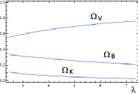
Figure 1: The density parameters of each component [$\Omega_{B}=$(the magentic field), $\Omega_{V}$ (the potential), and $\Omega_{K}$(the kinetic term of the scalar field)] for the case of $\alpha=\sqrt{6}$ and $\lambda>\alpha$. The power exponent of the scale factor is given by $p=(1+\lambda/\alpha)/2$.

We will show the stability condition later in §. IV.2.

III.2 The case with YM field

Now we show the dynamics changes when the YM interaction is turned on. Since we have the non-linear coupling in the YM field, a simple power-law ansatz may not work. But we first look for a solution similar to those found in the U(1) triplet case.

III.2.1 The case with the dominant electric component ${\rm(}E_{\scriptscriptstyle{\rm YM}}$)

If we assume $\rho_{E}\gg\rho_{B}$ but $\rho_{B}$ being non-vanishing due to the interaction between electric and magnetic fields, which we shall call the regime $E_{\scriptscriptstyle{\rm YM}}$, dropping the term with $\rho_{B}$, we find the same equations as the U(1) triplet case. As a result, we find the same solution [Eqs. (20)-(22)] as long as the electric component stays dominant. Under the conditions $\lambda<-\alpha$ and $\alpha(\alpha-\lambda)>4$, we obtain the power-law inflationary solution. Note that an accelerated expansion is possible even if $\alpha>\sqrt{2}$ just as was the case for the U(1) triplet electric type inflationYamamoto .

However, the situation in the case of YM field is not exactly the same as that for the U(1) triplet fields. In the above analysis, we have ignored the magnetic component, which is valid in the U(1) triplet case because the electric and magnetic fields are decoupled. However, the electric and magnetic components are always coupled in the YM field. Then we have to check whether the magnetic component is always negligible or not when it is initially small.

Since we assume the magnetic component is initially very small, we can solve the YM equation (7) dropping the term with $g_{\scriptscriptstyle{\rm YM}}$ (the magnetic contribution) as

$$\dot{A} = A_{1}a^{-1}e^{-\lambda\phi}={A_{1}\over a_{0}e^{\lambda\phi_{0}}}t^{-{\alpha+3\lambda\over 2\alpha}}\,,$$

$$A = A_{0}+{2\alpha A_{1}\over(\alpha-3\lambda)a_{0}e^{\lambda\phi_{0}}}t^{\alpha-3\lambda\over 2\alpha}\,,$$

where $A_{0}$ and $A_{1}$ are integration constants. Using this solution, we evaluate the ratio of two energy densities as

$${\rho_{B}\over\rho_{E}} \approx {\rho_{B}\over\rho_{E}}\Big{|}_{0}\left({a\over a_{0}}\right)^{4}\,,$$

where ${\rho_{B}/\rho_{E}}|_{0}$ is the initial value. We drop $A_{0}$ since we are interested in the asymptotic behavior ($t\rightarrow\infty$). As a result, if the magnetic component is initially sufficiently small, we have a power-law inflation just as the case with the Abelian multiple fields, but the contribution of the magnetic component gets larger during the evolution of the universe, and then the inflationary phase eventually ends because of the growth of the magnetic component. The e-folding time when the approximation becomes no longer valid is evaluated as

$$N_{\rm e\mathchar 45\relax folding} = \ln(a_{\rm end}/a_{0})$$

$$\approx -{1\over 4}\ln\left({\rho_{B}\over\rho_{E}}\Big{|}_{0}\right)\,.$$

For example, if we assume ${\rho_{B}/\rho_{E}}|_{0}=10^{-8}$, we find $N_{\rm e\mathchar 45\relax folding}\sim 4.6$. Hence unless the initial value of the magnetic energy density is extremely small, we do not find a sufficient e-folding number for the inflationary universe.

III.2.2 The case with the dominant magnetic component ${\rm(}B_{\scriptscriptstyle{\rm YM}}$)

We shall call it the regime $B_{\scriptscriptstyle{\rm YM}}$, when the magnetic component is much larger than the electric one. In this case the situation is not so simple as the U(1) case because we cannot ignore the non-linear term in (8) even if we assume $\rho_{E}\ll\rho_{B}$. Suppose we have the same solution as the U(1) case. We then evaluate $\dot{A}/A$ by the YM equation (7), which is now

$$\ddot{A}+{\alpha+5\lambda\over 2\alpha t}\dot{A}+2g_{\scriptscriptstyle{\rm YM}}^{2}{A^{3}\over a^{2}}=0\,.$$ (32)

We then find the asymptotic solution as

$$A=A_{\infty}\left[1+{4\alpha^{2}g_{\scriptscriptstyle{\rm YM}}^{2}A_{\infty}^{2}\over(\lambda-\alpha)(\alpha+3\lambda)}{t^{2}\over a^{2}}\right]\,,$$ (33)

which leads to

$${\dot{A}\over A}\approx{4\alpha g_{\scriptscriptstyle{\rm YM}}^{2}A_{\infty}\over(\alpha+3\lambda)a_{0}^{2}}t^{-\lambda/\alpha}$$ (34)

as $t\rightarrow\infty$. This ratio decays faster than $t^{-1}$, at which rate $4H\pm\lambda\dot{\phi}$ evolve in Eq. (8). So we can ignore the non-linear term with $\dot{A}/A$, which gives exactly the same equations as the $U(1)$ magnetic case.

As a result, we have the power-law solution just the same as in $B_{\rm U1}$. This solution is obtained asymptotically, and the non-linear term does not destroy it unlike the regime $E_{\scriptscriptstyle{\rm YM}}$ where the electric components dominate.

III.2.3 The case with both components

If both electric component and magnetic one are of equal magnitude, we cannot ignore either of them. Since it is a non-linearly coupled system, it is difficult to figure out what kind of solutions we expect. Although we need numerical studies, which we will give later, here we shall discuss one simple case, in which we assume the power-law behavior.

Suppose that the YM potential $A$ is a power-law function as $A\propto t^{s}$, and the scale factor and the scalar field are given by Eqs. (9) and (10). If the energy densities of the electric and magnetic fields are similar, i.e., $\rho_{E}\sim\rho_{B}$, we find $s=p-1$, and then

$$\rho_{E}\sim\rho_{B}\propto t^{-2}\times t^{-2(1-\lambda/\alpha)}\,.$$

Inserting this behavior into the YM equation (7), we find

$$2(p-1)\left(p-1+{\lambda\over\alpha}\right)+2g_{\scriptscriptstyle{\rm YM}}^{2}\left({A_{0}\over a_{0}}\right)^{2}=0\,,$$

which implies

$$2(p-1)\left(p-1+{\lambda\over\alpha}\right)<0\,.$$

For the power-law inflation ($p>1$), we have

$$1-{\lambda\over\alpha}>p>1\,.$$

As a result, $\rho_{E}\sim\rho_{B}$ drops faster than $\propto t^{-2}$, which is the scaling of energy density of the scalar field. Hence the contribution of YM field becomes less important as $t\rightarrow\infty$. It appears that it is not possible to find a power-law inflation with a significant residual $\rho_{E}\sim\rho_{B}$. Here, we find the power-law expansion only by a scalar field. An accelerated expansion is possible if $\alpha<\sqrt{2}$, as the conventional power-law inflation.

In the next section, we will give more details of interesting solutions in the present system including the inflationary solutions we have found and analyze their stability as fixed points in a dynamical system.

IV Stability Analysis

IV.1 Dynamical System

In order to analyze the dynamical behavior of our solutions found in §. III.2, we rewrite the basic equations in the form of a first order autonomous system. The inflationary solutions discussed in the previous sections, along with other interesting ones, appear as fixed points in the dynamical system. This allows us to study their local stability and reveal a complicated dynamical behavior that goes beyond the simple power-law time-dependence. We shall change the time coordinate from $t$ to the e-folding number $N=\ln(a/a_{0})$, and introduce new variables normalized by the Hubble expansion rate $H$ as

$${\cal E} = e^{{\lambda\over 2}\phi}{E\over H}=-e^{{\lambda\over 2}\phi}{A^{\prime}\over a}$$ (35)

$${\cal B} = e^{{\lambda\over 2}\phi}{B\over H}={\cal A}^{2}\,,$$ (36)

$${\cal A} = g_{\scriptscriptstyle{\rm YM}}^{1/2}e^{{\lambda\over 4}\phi}{A\over H^{1/2}a}\,.$$ (37)

Primes denote differentiations with respect to the e-folding number $N$. We then introduce the density parameter of the YM field as

$$\Omega_{\scriptscriptstyle{\rm YM}} = {\rho_{\scriptscriptstyle{\rm YM}}\over 3H^{2}}=\frac{1}{2}\left(\mathcal{E}^{2}+\mathcal{B}^{2}\right)\,,$$ (38)

and those of the potential and the kinetic energy of the scalar field as

$$\Omega_{V} = {V\over 3H^{2}}\,,$$ (39)

$$\Omega_{K} = {\dot{\phi}^{2}\over 6H^{2}}={\varpi^{2}\over 6}\,,$$ (40)

where $\varpi:=\dot{\phi}/H=\phi^{\prime}$. We also use

$$\Delta = {\rho_{B}-\rho_{E}\over\rho_{\scriptscriptstyle{\rm YM}}}\,,$$ (41)

which describes the difference of the fractions of the magnetic and electric components. It enables a unified treatment of electric- and magnetic-dominant regimes and also makes the asymmetry clear when the YM coupling comes into play. $\Delta=1$ and $-1$ correspond to the regime $B_{\scriptscriptstyle{\rm YM}}$ and $E_{\scriptscriptstyle{\rm YM}}$, respectively.

The Friedmann equation (2) now reads

$$\Omega_{K}+\Omega_{V}+\Omega_{\scriptscriptstyle{\rm YM}}=1\,.$$ (42)

The equation for the scalar field (6) is

$$\varpi^{\prime}={1\over 2}\left(6-\varpi^{2}\right)\left(\alpha-\varpi\right)+\left[2\varpi-3\left(\alpha+\lambda\Delta\right)\right]\Omega_{\scriptscriptstyle{\rm YM}}\,.$$ (43)

where we have used the Friedmann equation (42) to eliminate $\Omega_{V}$. The equations for the YM field (8) are now

$${\cal A}^{\prime} = {1\over 4}\left[\varpi(\varpi+\lambda)-4\left(1-\Omega_{\scriptscriptstyle{\rm YM}}\right)\right]{\cal A}-\Gamma{\cal E}$$ (44)

$${\cal E}^{\prime} = {1\over 2}\left[\varpi(\varpi-\lambda)-4\left(1-\Omega_{\scriptscriptstyle{\rm YM}}\right)\right]{\cal E}+2\Gamma{\cal A}^{3}\,.$$ (45)

where

$$\Gamma=g_{\scriptscriptstyle{\rm YM}}^{1/2}e^{-{\lambda\over 4}\phi}H^{-1/2}\,,$$ (46)

whose evolution equation is

$$\Gamma^{\prime} = {1\over 4}\left[\varpi(\varpi-\lambda)+4\Omega_{\scriptscriptstyle{\rm YM}}\right]\Gamma\,.$$ (47)

This auxiliary quantity $\Gamma$ is the “normalized” YM coupling in the sense that the subsystem defined by $\Gamma=0$ corresponds to the dynamical system that describes homogeneous and isotropic $U(1)$ triplet fields. The YM equations (44) and (45) are rewritten in terms of the denisty parameter $\Omega_{\scriptscriptstyle{\rm YM}}$ and the ratio $\Delta$ as

$$\Omega_{\scriptscriptstyle{\rm YM}}^{\prime} = \left[-4+\varpi(\varpi+\lambda\Delta)+4\Omega_{\scriptscriptstyle{\rm YM}}\right]\Omega_{\scriptscriptstyle{\rm YM}}$$ (48)

$$\Delta^{\prime} = \lambda\varpi\left(1-\Delta^{2}\right)-4\epsilon\Gamma\left(1-\Delta\right)^{1\over 2}\left(1+\Delta\right)^{3\over 4}\Omega_{\scriptscriptstyle{\rm YM}}^{1\over 4}\,,$$ (49)

where $\epsilon={\rm sign}({\cal A}{\cal E})$. We then find the dynamical system in a closed form. Since the physical interpretation of the normalized vector potential $\mathcal{A}$ is not clear, we take Eqs. (43), (48), (49) and (47) with the Hamiltonian constraint (= the Friedmann equation) (42) as the basic equations to analyze the stability around the fixed points. The drawback is the appearance of $\epsilon$ which takes into account the ambiguity inherent to taking square roots. This causes a problem in the numerical study in the next section when the system undergoes oscillations. For this reason, Eqs. (44) and (45) instead of Eqs. (48) and (49) are used there.

IV.2 The case with U(1) triplet fields

Before going into analysis of our system, for an introduction and a comparison, we first summarize the case with the U(1) triplet fields, which was discussed in Yamamoto , using the present dynamical variables. To make a clear distinction, we replace $\Omega_{\rm YM}$ with $\Omega_{\rm U1}$. Now $\Delta=1$ and $-1$ correspond to the regimes $B_{\rm U1}$ and $E_{\rm U1}$ respectively.

In the case with the U(1) triplet fields, the dynamical system is obtained by setting $\Gamma=0$ in the above;

$$\varpi^{\prime} = {1\over 2}\left(6-\varpi^{2}\right)\left(\alpha-\varpi\right)$$

$$~{}~{}+\left[2\varpi-3\left(\alpha+\lambda\Delta\right)\right]\Omega_{\rm U1}$$

$$\Omega_{\rm U1}^{\prime} = \left[-4+\varpi^{2}+\lambda\varpi\Delta+4\Omega_{\rm U1}\right]\Omega_{\rm U1}$$

$$\Delta^{\prime} = \lambda\varpi\left(1-\Delta^{2}\right)\,.$$

If $\varpi\neq 0$ and $\Omega_{\rm U1}\neq 0$, the fixed points are classified into two cases; $\Delta=-1$ (the case with the electric field) and $\Delta=1$ (the case with the magnetic field). In each case, we find two fixed points as follows:

$$(a) \varpi=-3\lambda\Delta\,,~{}~{}\Omega_{\rm U1}={2-3\lambda^{2}\over 2}\,,$$

$$(b) \varpi={4\over\alpha+\lambda\Delta}\,,~{}~{}\Omega_{\rm U1}={\alpha(\alpha+\lambda\Delta)-4\over(\alpha+\lambda\Delta)^{2}}\,.~{}~{}~{}~{}$$

Since the density parameters are positive definite, $\lambda\leq\sqrt{2/3}$ for the fixed point ($a$) to exist. In this case, $\Omega_{V}=0$, which means that either the potential is absent from the beginning or the potential becomes asymptotically negligible compared with the kinetic term $\varpi^{2}/2$.

From a perturbative analysis, we can check the stability of these fixed points. For the fixed points ($a$), we find that at least the eigenvalue for the perturbation of $\Delta$ is always positive ($\omega_{\Delta}=6\lambda^{2}$). Hence it is unstable. Hereafter, we use $\omega$ to denote eigenvalues with subscripts indicating the variable to which the eigenvalue is associated.

The fixed points ($b$) represent the power-law solutions ($E_{\rm U1}$ and $B_{\rm U1}$) found in §. III.1. The perturbative analysis gives the following three eigenvalues:

$$\omega_{\Delta}=-{8\lambda\Delta\over\alpha+\lambda\Delta}$$ (50)

and the two roots of the quadratic equation

$$(\alpha+\lambda\Delta)^{2}\omega^{2}+(\alpha+\lambda\Delta)(\alpha+3\lambda\Delta)\omega$$

$$+[\alpha(\alpha+\lambda\Delta)-4][4+3\lambda\Delta(\alpha+\lambda\Delta)]=0\,,$$

from the perturbations of $\varpi$ and $\Omega_{\scriptscriptstyle{\rm YM}}$.

From the existence conditions given by Eq. (25) or Eq.(31), we have $\alpha(\alpha+\lambda\Delta)-4>0$. Hence, if and only if $\lambda\Delta>0$ is satisfied, all the three eigenvalues are negative (or the real parts are negative if they are complex). As a result, the solution with the conditions

$$\lambda\Delta>0\,,~{}~{}\alpha(\alpha+\lambda\Delta)-4>0$$ (51)

is stable against linear perturbations. More concretely, the stability conditions for the cases with the electric field ($E_{\rm U1}$) and magnetic field ($B_{\rm U1}$) are given by,

$$\lambda<0\,,~{}~{}\alpha(\alpha-\lambda)>4\,,$$ (52)

$$\lambda>0\,,~{}~{}\alpha(\alpha+\lambda)>4\,,$$ (53)

respectively. If $\lambda>0$, the magnetic power-law solution (Eqs. (9), (10) and (12) with (26) and (28) ) is always an attractor in the parameter range of $\alpha(\alpha+\lambda)>4$, while if $\lambda<0$ the electric power-law solution (Eqs. (9), (10) and (12) with (20) and (22) ) is always an attractor in the parameter range of $\alpha(\alpha-\lambda)>4$.

For the rest of the parameter space ($\alpha-4/\alpha<\lambda<-\alpha+4/\alpha$), the attractor is a fixed point with $\Omega_{\rm U1}=0$, where the scalar field dominates the universe. The fixed point, which we denote $S_{\rm U1}$, is given by

$$\varpi=\alpha\,,~{}~{}\Omega_{\rm U1}=0\,,~{}~{}\Delta=\pm 1\,.$$ (54)

The perturbative analysis gives the three eigenvalues as

$$\omega_{\varpi} = -{1\over 2}(6-\alpha^{2})\,,$$

$$\omega_{\Omega_{\rm U1}} = \alpha(\alpha+\lambda\Delta)-4\,,$$

$$\omega_{\Delta} = -2\alpha\lambda\Delta\,.$$

Hence the power-law solution driven only by the scalar field is stable if $\lambda\Delta>0$ and $\alpha(\alpha+\lambda\Delta)-4<0$. Between the two solutions with alternative sings, the stable one is

$$\varpi=\alpha\,,~{}~{}\Omega_{\rm U1}=0\,,~{}~{}\Delta=1\,.$$ (55)

for $\lambda>0$, while

$$\varpi=\alpha\,,~{}~{}\Omega_{\rm U1}=0\,,~{}~{}\Delta=-1\,.$$ (56)

for $\lambda<0$.

We summarize the result for the U(1) triplet case in Fig. 2 and in Table 1:

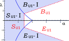
Figure 2: The parameter range for power-law solutions in the case with the U(1) triplet fields. The inflationary attractors are indicated by black letters while non-inflationary attractors are red. The attractor solution with the electric field is given for $\lambda<0$ and $\alpha(\alpha-\lambda)>4$ ($E_{\rm U1}$), while one with the magnetic field is for $\lambda>0$ and $\alpha(\alpha+\lambda)>4$ ($B_{\rm U1}$) . In the range of $\alpha-4/\alpha<\lambda<-\alpha+4/\alpha$ ($S_{\rm U1}$), we find the attractor dominated by the scalar field. All inflationary solutions are stable. The inflation with the U(1) triplet field is found in the range either of $\lambda<-\alpha$ and $\alpha(\alpha-\lambda)>4$ ($E_{\rm U1}$-I:with the electric field) or of $\lambda>\alpha$ and $\alpha(\alpha+\lambda)>4$ ($B_{\rm U1}$-I:with the magnetic field). The conventional power law inflation with an exponential potential is possible only for $\alpha<\sqrt{2}$ and $\alpha-4/\alpha<\lambda<-\alpha+4/\alpha$. ($S_{\rm U1}$-I)

fixed point	$S_{\rm U1}$	$E_{\rm U1}$	$B_{\rm U1}$
existence	$\alpha<\sqrt{6}$	$\alpha-{4/\alpha}>\lambda$	$-\alpha+{4/\alpha}<\lambda$
$p$	${2/\alpha^{2}}$	${1\over 2}\left(1-{\lambda/\alpha}\right)$	${1\over 2}\left(1+{\lambda/\alpha}\right)$
$\Omega_{\scriptscriptstyle{\rm YM}}$	$0$	${\alpha(\alpha-\lambda)-4\over(\alpha-\lambda)^{2}}$	${\alpha(\alpha+\lambda)-4\over(\alpha+\lambda)^{2}}$
$\Omega_{V}$	$1-{\alpha^{2}/6}$	${4-3\lambda(\alpha-\lambda)\over 3(\alpha-\lambda)^{2}}$	${4+3\lambda(\alpha+\lambda)\over 3(\alpha+\lambda)^{2}}$
$\Omega_{\rm K}$	${\alpha^{2}/6}$	${8\over 3(\alpha-\lambda)^{2}}$	${8\over 3(\alpha+\lambda)^{2}}$
stability	$\alpha-{4/\alpha}<\lambda<-\alpha+{4/\alpha}$	$\lambda<0$	$\lambda>0$
inflation	$\alpha<\sqrt{2}$       ($S_{\rm U1}$-I)	$\lambda<-\alpha$   ($E_{\rm U1}$-I)	$\lambda>\alpha$   ($B_{\rm U1}$-I)

Table 1: The fixed points and their properties for the case with U(1) triplet fields. The second row gives the existence conditions. The bottom two rows are understood to hold when those existence conditions are satisfied.

IV.3 Important Fixed Points in the dynamical system with YM field

Now we move on to include the non-linear YM interaction. The non-trivial fixed points are classified into two cases: $\Gamma=0$ and $\Gamma\neq 0$. In the former case, we find the same fixed points as the U(1) triplet case, although their stability is different as we will show later. The latter case gives new fixed points, which do not exist in the U(1) triplet system.

Note that a fixed point may not be found by an exact solution, but can be reached as a certain limit. For example, the fixed points with $\Gamma=0$ would imply either $g_{\rm YM}=0$ or $He^{\lambda\phi/2}=\infty$, neither of which is of interest in our analysis here. However, starting from $g_{\rm YM}\neq 0$ and finite $H$ and $\phi$, the system may approach $\Gamma\rightarrow 0$ asymptotically as $t\rightarrow\infty$. From the mathematical point of view, those fixed points are well-defined and a part of the dynamical system and we include them in the following analysis.

IV.3.1 $\Gamma=0$

In this case, which should reproduce the fixed points of the previous subsection, we can classify the solutions into two cases: $\Omega_{\scriptscriptstyle{\rm YM}}=0$ and $\Omega_{\scriptscriptstyle{\rm YM}}\neq 0$.

(a) $\Omega_{\scriptscriptstyle{\rm YM}}=0$
In the case with $\Omega_{\scriptscriptstyle{\rm YM}}=0$, the scalar field energy is dominant. From (43), we find either $\varpi^{2}=6$ or $\varpi=\alpha$ with $\Delta^{2}=1$. The former fixed point corresponds to the case that the kinetic energy of the scalar field is dominant, which is unstable against perturbations. The latter fixed points denote the power-law expanding universe with an exponential potential (the counterpart of $S_{\rm U1}$) and will be called $S_{\rm YM}$. The ratio of the potential energy $V$ to the kinetic energy is $(6-\alpha^{2})/\alpha^{2}$. As is well known, these fixed points are attractors if $\alpha\leq\sqrt{6}$ for the case only with a scalar field.

In the present case, because of the YM field, the stability condition changes as follows. The linearized equations for these fixed points give four eigenvalues:

$$\omega_{\varpi} = {1\over 2}\left(\alpha^{2}-6\right)\,,$$ (57)

$$\omega_{\Omega_{\scriptscriptstyle{\rm YM}}} = \alpha\lambda\Delta+\alpha^{2}-4\,,$$ (58)

$$\omega_{\Delta} = -2\alpha\lambda\Delta\,,$$ (59)

$$\omega_{\Gamma} = {1\over 2}\alpha(\alpha-\lambda)\,.$$ (60)

Three eigenvalues (57), (58), and (59) are all negative if $\lambda>0$ and $\lambda<-\alpha+4/\alpha$ for $\Delta=1$, or if $\lambda<0$ and $\lambda>\alpha-4/\alpha$ for $\Delta=-1$. The forth eigenvalue (60) becomes negative if $\lambda>\alpha$. As a result, the fixed point with $\Delta=1$ is stable in the parameter range of $\alpha<\lambda<-\alpha+4/\alpha$.

On the other hand, taking $\lambda<\alpha$ gives instability against the perturbations of $\Gamma$. However, as long as $\Omega_{\rm YM}$ stays small, the growing $\Gamma$ does not disturb the evolution of the universe as well as the dynamics of the scalar field since $\Gamma$ does not appear explicitly in Eqs. (42) and (43). This is indeed the case when $\alpha-4/\alpha<\lambda<\alpha$. As we shall confirm later in the numerical analysis, the dynamics of the universe is dominated by the scalar field and accurately described by the fixed point discussed here, despite the apparent instability in the eigenvalue $\omega_{\Gamma}$. The exponentially increasing $\Gamma$ only triggers a rapid oscillation for the perturbed YM field whose amplitude remains small.

In summary, we conclude that these fixed points are stable in the range $\alpha-4/\alpha<\lambda<-\alpha+4/\alpha$ as was found for $S_{\rm U1}$. Nevertheless, there is a distinction between $S_{\rm U1}$ and $S_{\rm YM}$ for $\lambda<\alpha$ with the dynamics of the YM field being different.

(b) $\Omega_{\scriptscriptstyle{\rm YM}}\neq 0$
For the case with $\Omega_{\scriptscriptstyle{\rm YM}}\neq 0$, the YM field plays an important role in the dynamics of the universe. We find $\Delta=\pm 1$ unless $\varpi=0$, for which we do not have any interesting dynamics.

$\Delta=-1$ and $1$ correspond to the case of the electric component dominance ($E_{\scriptscriptstyle{\rm YM}}$) and that of the magnetic component dominance ($B_{\scriptscriptstyle{\rm YM}}$), respectively. As we have already mentioned, the YM field always consists of both components. Hence these fixed points are reached only asymptotically, if they are stable. Just the same as the U(1) triplet fields, we find two fixed points for each case. However, one of them with $\varpi=-3\lambda\Delta$ is unstable. Hence we discuss the other cases:

$$(1) \Delta=1~{}~{}(B_{\scriptscriptstyle{\rm YM}})$$ (61)

$$~{}~{}\varpi={4\over\alpha+\lambda}\,,~{}~{}$$

$$~{}~{}\Omega_{\scriptscriptstyle{\rm YM}}={\alpha(\alpha+\lambda)-4\over(\alpha+\lambda)^{2}}\,.$$

$$(2) \Delta=-1~{}~{}(E_{\scriptscriptstyle{\rm YM}})$$ (62)

$$~{}~{}\varpi={4\over\alpha-\lambda}\,,~{}~{}$$

$$~{}~{}\Omega_{\scriptscriptstyle{\rm YM}}={\alpha(\alpha-\lambda)-4\over(\alpha-\lambda)^{2}}\,.~{}~{}~{}~{}~{}~{}$$

These fixed points correspond to the solutions with the magnetic component and the electric one found in §. III.1.3 and III.1.2, respectively.

Without the non-linear interaction, these points were symmetric: they were related by the electromagnetic duality and had the same stability properties. The YM coupling skews the symmetry.

For the case (1), the eigenvalues are given by

$$\omega_{\Delta} = -{8\lambda\over\alpha+\lambda}$$ (63)

$$\omega_{\Gamma} = {2(\alpha-\lambda)\over\alpha+\lambda}$$ (64)

and the two roots of the algebraic equation

$$(\alpha+\lambda)^{2}\omega^{2}+(\alpha+\lambda)(\alpha+3\lambda)\omega$$

$$~{}~{}+[\alpha(\alpha+\lambda)-4][4+3\lambda(\alpha+\lambda)]=0\,.~{}~{}~{}~{}~{}$$ (65)

We find all eigenvalues are negative if and only if $\lambda>\alpha$ and $\alpha(\alpha+\lambda)-4>0$ are satisfied. Since this condition corresponds to the power-law inflationary solution with YM field, we can conclude that the power-law inflationary solution with magnetic component dominance ($B_{\rm YM}$-I) is an attractor. The difference from the U(1) multiplet case is that the solutions in the parameter range of $0<\lambda<\alpha$, which are not inflationary, are no longer an attractor. We will discuss later which asymptotic state we find in this region.

On the other hand, in the case with $\Delta=-1$, the eigenvalues are given by

$$\omega_{\Delta} = {8\lambda\over\alpha-\lambda}$$ (66)

$$\omega_{\Gamma} = 2$$ (67)

and the two roots of the algebraic equation

$$(\alpha-\lambda)^{2}\omega^{2}+(\alpha-\lambda)(\alpha-3\lambda)\omega$$

$$~{}~{}+[\alpha(\alpha-\lambda)-4][4+3\lambda(\alpha-\lambda)]=0\,.~{}~{}~{}~{}~{}$$ (68)

We find that three eigenvalues are negative for the power-law inflationary solution as long as $\lambda<-\alpha$ and $\alpha(\alpha-\lambda)-4>0$, but one eigenvalue $\omega_{\Gamma}$, which corresponds to the perturbations of $\Gamma$ (non-linear interaction term of the YM field), is always positive and does not depend on any parameters. This is the same behavior which we have seen in §.III.2.1. As a result, this solution is unstable and the typical instability time scale is O(1) e-folding time since the present time coordinate is $N=\ln(a/a_{0})$ and therefore $\Gamma\propto\exp\left(\omega_{\Gamma}N\right)$. If the magnetic component is initially sufficiently small, we may find this power-law inflation solution by the electric components in the beginning, but the orbit leaves it just after $O(1)$ e-folding time. We conclude that the power-law inflationary solution with the electric component dominance $E_{\rm YM}$-I is unstable, contrary to the $E_{\rm U1}$.

IV.3.2 $\Gamma\neq 0$

Here we assume that $\Omega_{\scriptscriptstyle{\rm YM}}\neq 0$ because $\Gamma$ becomes important when the YM field gives non-trivial contribution to the cosmic expansion. Note that $\Delta^{2}=1$ ($E_{\scriptscriptstyle{\rm YM}}$ or $B_{\scriptscriptstyle{\rm YM}}$) is no longer a fixed point. We find the following two non-trivial fixed points, if $\lambda^{2}\geq 6$:

$$\varpi=\varpi^{(\pm)}:={3\over 2}\left(\lambda\pm\sqrt{\lambda^{2}-16/3}\right)$$

The values at both fixed points can be described neatly by the deceleration parameter

$$q^{(\pm)}:=1+{\left(\varpi^{(\pm)}\right)^{2}\over 6}={\lambda\varpi^{(\pm)}\over 2}-1\,,$$ (69)

as

$$\Omega_{\scriptscriptstyle{\rm YM}}^{(\pm)}=2-q^{(\pm)}\,,~{}~{}\Delta^{(\pm)}={1-q^{(\pm)}\over 1+q^{(\pm)}}\,,~{}~{}$$

$$\Gamma^{(\pm)}=\left[{(q^{(\pm)})^{2}(1+q^{(\pm)})\over 2(2-q^{(\pm)})}\right]^{1/4}\,,$$

$$p^{(\pm)}={1\over q^{(\pm)}+1}\,.$$

Note that $\Omega_{V}=0$ at these fixed points and they are unique to the YM case. From (69) and the positivity of the density parameter $\Omega_{\scriptscriptstyle{\rm YM}}\geq 0$, we find

$$1\leq q^{(\pm)}\leq 2\,.$$ (70)

Hence the power exponent of the scale factor $p^{(\pm)}$ is

$$1/3\leq p^{(\pm)}\leq 1/2\,,$$

which is between a radiation dominant state and a stiff-matter dominant one.

The perturbative analysis is common to both of the fixed points $\lambda\geq\sqrt{6}$ ($NA_{+}$) and $\lambda\leq-\sqrt{6}$ ($NA_{-}$). We find the following eigenvalues;

$$\omega_{\Omega_{\scriptscriptstyle{\rm YM}}\mathchar 45\relax\varpi} = 2\left(1-{\alpha\over\lambda}\right)(q+1)\,,$$

$$\omega_{\Gamma\mathchar 45\relax\Delta} = q-2\,,$$

which are associated with the eigen vectors $\delta\Omega_{\scriptscriptstyle{\rm YM}}+(\varpi/3)\delta\varpi$ and $\delta\Gamma/\Gamma-[(q-2)(q+1)/8q]\delta\Delta$, respectively, and the two roots of the quadratic equation

$$\omega^{2}+(2-q)\omega+{4q(3-q)\over q-1}=0\,.$$

Since $q$ is in the range of (70), if $0<\lambda<\alpha$, we find all eigenvalues are negative, which means $NA_{+}$ is stable. On the other hand, $\omega_{\Omega_{\rm YM}\mathchar 45\relax\varpi}$ turns positive when $\lambda<0$ and we find $NA_{-}$ is unstable. As a result, we find a stable fixed point in the parameter range of $\sqrt{6}<\lambda<\alpha$ ($NA_{+}$), which partly takes care of the lost stability of $B_{\rm YM}$ in the region $\lambda<\alpha$.

We summarize our result for the SU(2) YM field in Fig. 3 and in Table 2:

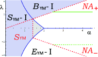
Figure 3: The parameter range for power-law solutions in the case with the YM field. The inflationary attractor solution with the magnetic component is found for $\alpha<\lambda<-\alpha+4/\alpha$ ($B_{\scriptscriptstyle{\rm YM}}$-I). On the other hand, the inflationary solution with the electric component, which is found in the range of $\alpha-4/\alpha<\lambda<-\alpha$ ($E_{\scriptscriptstyle{\rm YM}}$-I), is unstable. In the range of $\alpha-4/\alpha<\lambda<-\alpha+4/\alpha$ ($S_{\scriptscriptstyle{\rm YM}}$), we find the attractor solutions dominated by a scalar field. For inflation, we need an additional condition $\alpha<\sqrt{2}$ ($S_{\scriptscriptstyle{\rm YM}}$-I). We also find new fixed points $NA_{\pm}$, which exist only for non-Abelian gauge fields.

	$S_{\scriptscriptstyle{\rm YM}}$	$E_{\scriptscriptstyle{\rm YM}}$	$B_{\scriptscriptstyle{\rm YM}}$	$NA_{+}$	$NA_{-}$
existence	$\alpha<\sqrt{6}$	$\alpha-4/\alpha>\lambda$	$\lambda>-\alpha+{4/\alpha}$	$\sqrt{6}<\lambda$	$\lambda<-\sqrt{6}$
$p$	${2/\alpha^{2}}$	${1\over 2}\left(1-{\lambda/\alpha}\right)$	${1\over 2}\left(1+{\lambda/\alpha}\right)$	${1\over 4\lambda}(\lambda+\sqrt{\lambda^{2}-16/3})$	${1\over 4\lambda}(\lambda-\sqrt{\lambda^{2}-16/3})$
$\Omega_{\scriptscriptstyle{\rm YM}}$	$0$	${\alpha(\alpha-\lambda)-4\over(\alpha-\lambda)^{2}}$	${\alpha(\alpha+\lambda)-4\over(\alpha+\lambda)^{2}}$	${3\over 4}(4-\lambda^{2}+\lambda\sqrt{\lambda^{2}-16/3})$	${3\over 4}(4-\lambda^{2}-\lambda\sqrt{\lambda^{2}-16/3})$
$\Omega_{V}$	$1-{\alpha^{2}/6}$	${4-3\lambda(\alpha-\lambda)\over 3(\alpha-\lambda)^{2}}$	${4+3\lambda(\alpha+\lambda)\over 3(\alpha+\lambda)^{2}}$	0	0
$\Omega_{\rm K}$	${\alpha^{2}/6}$	${8\over 3(\alpha-\lambda)^{2}}$	${8\over 3(\alpha+\lambda)^{2}}$	${3\over 4}(\lambda^{2}-8/3-\lambda\sqrt{\lambda^{2}-16/3})$	${3\over 4}(\lambda^{2}-8/3+\lambda\sqrt{\lambda^{2}-16/3})$
stability	$\alpha-4/\alpha<\lambda<-\alpha+4/\alpha$	always unstable	$\alpha<\lambda$	$\lambda<\alpha$	always unstable

Table 2: The fixed points and their properties for the case with YM fields. Stability of $S_{\rm YM}$ takes into account the fact that unstable $\Gamma$ does not destroy the dominance of the scalar field. $NA_{\pm}$ cannot be inflationary. Inflationary conditions for the other points are the same as the $U(1)$ triplet case.

V Numerical Study

From the above stability analysis, we find there are stable attractors if $\lambda\geq\alpha$ ($B_{\scriptscriptstyle{\rm YM}}$-I) or $\alpha\geq\lambda\geq\sqrt{6}$ ($NA_{+}$). We also find that a scalar field dominated universe ($S_{\scriptscriptstyle{\rm YM}}$), which is the same as the stable attractor in the model with a scalar field with an exponential potential ($V=V_{0}\exp(-\alpha\phi)$), is stable in the parameter range of $\alpha-4/\alpha\leq\lambda\leq-\alpha+4/\alpha$, even though the YM field does not necessarily settle down to its attractor state. As we will show here, it will oscillate in this scalar dominated background.

We may also wonder what is the future asymptotic behavior for the other range of the coupling parameters $\alpha$ and $\lambda$, i.e., $\lambda>\alpha$ and $\lambda<\sqrt{6}$. Numerical calculations give us some insight into this question too.

Numerical study also tells us strengths of the stable attractors. Since our stability analysis is based on the linear perturbations, we need numerical analysis to know how the attractor state is achieved from generic initial data.

V.1 Numerical Analysis

V.1.1 Stable attractors

We begin with a small value of $\alpha$ for which the conventional power-law inflation is known to occur in the absence of gauge-kinetic coupling, namely $\alpha<\sqrt{2}$.

We choose the representative value to be $\alpha=1$. We first performed the calculation for $\lambda=2$ (see Fig. 4), which shows the conventional power-law inflation with an exponential potential ($S_{\scriptscriptstyle{\rm YM}}$-I ). The YM field energy drops quickly. We find that the asymptotic power exponent of the scale factor is 2, which is consistent with the value of the conventional power-law inflation ($p=2/\alpha^{2}$).

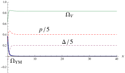
Figure 4: Inflation for $\alpha=1,\lambda=2$. This case obeys the usual cosmic-no-hair.

When $\lambda>3$, our analysis suggests the power-law inflation assisted by the magnetic component of the YM field ($B_{\scriptscriptstyle{\rm YM}}$-I) is a stable attractor of the system. Fig.5 confirms this fact as the density parameter for magnetic component stays constant ($\Omega_{\scriptscriptstyle{\rm YM}}$=constant and $\Delta=1$) while the scalar potential dominates the energy budget, which implies the universe undergoes accelerated expansion. An important difference between Figs.4 and 5 is that the acceleration is actually stronger when $\Omega_{\rm YM}$ does not vanish. We indeed find the asymptotic value of the power exponent $p$ is 3 instead of 2.

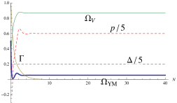
Figure 5: Occurrence of inflation assisted by the magnetic field for $\alpha=1,\lambda=5$. Convergence to the inflating attractor $B_{\scriptscriptstyle{\rm YM}}$-I is clearly seen.

We deliberately chose the initial condition such that the scalar kinetic energy and the electric component are dominant over the others and the effect of YM coupling is significant. As shown in Fig.5, $\Delta$ approaches unity and $\Gamma$ decays quickly whereby the system essentially reduces to the $U(1)$ triplet model. We find $B_{\scriptscriptstyle{\rm YM}}$-I asymptotically.

Next, we take a negative $\lambda$ and confirm the electric-magnetic asymmetry for non-Abelian gauge fields. Fig.6 exhibits two different regimes. In the beginning, the electric energy density grows according to the linear instability caused by the strong gauge-kinetic coupling and the system is attracted towards the power-law inflation assisted by electric component of the YM field ($E_{\scriptscriptstyle{\rm YM}}$-I).

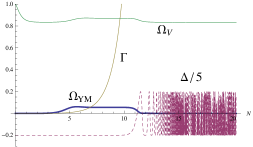
Figure 6: Inflation $S_{\scriptscriptstyle{\rm YM}}$-I with electromagnetic oscillation via the electric YM inflation ($E_{\scriptscriptstyle{\rm YM}}$-I) for $\alpha=1,\lambda=-5$. The initial value of the ratio of the energy density of the magnetic component to that of the electric one is $10^{-8}$. Between $5<N<10$, $\Omega_{V}$ is greater than its final value, which means the acceleration is stronger during that period thanks to the help by the electric component. As $\Gamma$ gets to order unity, this regime is ruined and $\Omega_{\scriptscriptstyle{\rm YM}}$ decays while the fields oscillate.

During that period, however, $\Gamma$ continues to increase and eventually destroys the inflationary regime at $N\sim 10$. The transient inflation $E_{\scriptscriptstyle{\rm YM}}$-I continues for $5\sim 6$ e-folding number, which is consistent with our evaluation given in §. III.2.1.

After that, the universe is dominated by the scalar field while YM field is oscillating. In this case, since $\alpha$ is small enough to cause accelerated expansion by itself, this oscillation phase is also inflating. For comparison, we also show the plots with a smaller value of $|\lambda|$ (Fig.7). The behavior is similar to Fig. 6, but there is no transient regime of $E_{\scriptscriptstyle{\rm YM}}$-I.

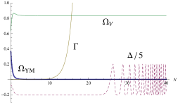
Figure 7: Inflation for $\alpha=1,\lambda=-2$. While the dynamics of the universe is entirely dominated by the scalar field, gauge fields oscillate at late time.

When $\lambda$ is negative, from the instability of $E_{\scriptscriptstyle{\rm YM}}$-I, there is a peculiar behavior of rapid oscillation at late time between electric and magnetic components, which is not seen for positive $\lambda$.

Let us turn our attention to the supportive role of gauge fields in realizing inflation. We take $\alpha=2$ for which inflation is impossible by the scalar field itself. With $\lambda=5$, we obtain Fig. 8 where $\Delta=1$ in the future asymptotic state. The value of $\Omega_{V}$ close to unity shows the expansion is accelerated, which can also be seen by the power exponent $p>1$.

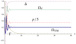
Figure 8: Inflation assisted by the YM field ($B_{\scriptscriptstyle{\rm YM}}$-I) for $\alpha=2,\lambda=5$. Note that the asymptotic value of $\Omega_{V}$ is sufficiently large to cause accelerated expansion. Although the slope of the scalar potential is not flat enough to maintain the potential domination by itself, the magnetic component of the YM field also takes up the scalar field energy and helps realizing the inflation.

As was investigated in the previous sections, this is due to the interaction between the scalar and YM fields that transfers scalar field energy to magnetic component of the YM field and slows down its rolling down the potential.

Note that the velocity of the scalar field is given by $\dot{\phi}=2\ln t/\alpha$, which is the same as the conventional power-law inflation. The difference is the values of total energy densities. The effective potential in the present model is given by the YM energy as well as the scalar potential $V$ (Eq. (14)), which gives a larger Hubble expansion rate. As a result, the velocity with respect to the e-folding number $N$ becomes slower as $\phi^{\prime}=\dot{\phi}/H$.

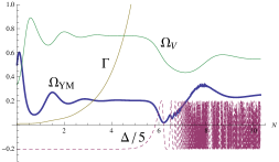
Figure 9: Inflation for $\alpha=2,\lambda=-5$. Intermediately ($2\lesssim N\lesssim 6$), the universe briefly inflates ($E_{\scriptscriptstyle{\rm YM}}$-I). Then $\Gamma$ eventually dictates the dynamics of the YM field.

For the $U(1)$ gauge fields, the same type of inflation with non-flat potential $E_{\rm U1}$-I could have been seen for negative $\lambda$ because of the electro-magnetic duality. In the present non-Abelian case, however, a negative $\lambda$ drives not only electric component but also the normalized gauge coupling $\Gamma$, by which the inflationary regime is made transient and the final state contains mixture of electric, magnetic and scalar fields (Fig.9). During the transient phase of inflation supported by the electric component of the YM field ($E_{\scriptscriptstyle{\rm YM}}$-I), one can see the values of $\Omega_{V}$ and $\Omega_{\scriptscriptstyle{\rm YM}}$ being the same as the corresponding magnetic inflation.

Finally, we confirm the stability of the new non-Abelian fixed point $NA_{+}$ for $\lambda>\sqrt{6}$ (Fig.10).

Figure 10: Convergence to the non-Abelian attractor $NA_{+}$ for $\alpha=4,\lambda=3$. It is distinct from the other plots in that $\Gamma$ settles down to a constant value.

The convergence is relatively slow and all the dynamical components undergo oscillations. In contrast to the other cases where $\Gamma$ either diverges or dies away, this parameter region sees convergence to an attractor value, which necessarily means negligible $\Omega_{V}$. Although it is not of interest in the context of inflation, it illustrates a distinct effect of the gauge coupling by forcing the potential term to vanish that would never happen in scalar-U(1) systems.

V.1.2 Oscillation of the YM field

The focus of this subsection is to understand the future asymptotic behavior of the system in the parameter region where the elementary fixed point analysis suggests there is no stable attractor solution. It turns out the nature of the dynamics in this regime is oscillation driven by the gauge coupling.

Fig.11 shows the occurrence of scalar-YM oscillation as the future asymptotic state of the dynamical system for $\alpha=4,\lambda=-3$. As is expected, the potential energy does not play a prominent role here. $\Omega_{V}$ and $\Omega_{\scriptscriptstyle{\rm YM}}$ appear to converge to finite values although the numerical calculation has not been able to confirm it due to the computational difficulty caused by the rapid oscillation of $\Delta$ and the ever-growing $\Gamma$.

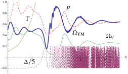
Figure 11: Oscillation for $\alpha=4,\lambda=-3$. As is expected, while $\Gamma$ is smaller than unity, the system approaches the fixed point with the electric component $E_{\scriptscriptstyle{\rm YM}}$. After the effect of non-linear gauge coupling kicks in, the dynamics is irregular at the beginning. It appears the oscillation of $\Omega_{V}$ and $\Omega_{\scriptscriptstyle{\rm YM}}$ eventually die away, finding some asymptotic solution with the YM field oscillations. The power exponent $p$ of the scale factor is slightly larger than $1/2$.

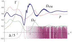
Figure 12: Oscillation for $\alpha=4,\lambda=-2$. Qualitatively the same dynamics as $\lambda=-3$. The only essential difference from Fig.11 is the asymptotic value of $\Omega_{V}$ and $\Omega_{\scriptscriptstyle{\rm YM}}$.

The behavior is mostly the same for negative $\lambda$ regardless of $\lambda<-\sqrt{6}$ or not (Fig.12). The power exponent $p$ of the scale factor is always slightly larger than $1/2$.

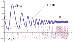
Figure 13: Oscillation for $\alpha=4,\lambda=2$. One can see the exponentially decaying amplitude of oscillation for $\Omega_{\scriptscriptstyle{\rm YM}}$. In contrast to $\lambda<0$, the scalar potential contribution becomes completely negligible.

In contrast, $\lambda=\sqrt{6}$ is a threshold value for positive $\lambda$ since the YM fixed point becomes the attractor above it (see Fig.10). Below the critical value, the asymptotic dynamics is rather analogous to the cases with negative $\lambda$, but with a significantly smaller contribution of $\Omega_{V}$. Convergence to an asymptotic value for $\Omega_{\scriptscriptstyle{\rm YM}}$ can be seen more clearly here (Fig.13). The power exponent $p$ of the scale factor is slightly smaller than $1/2$ for $\lambda>0$.

V.2 Asymptotic spacetime with the oscillation of the YM field

From our numerical study, we find that the universe still approaches some attractor spacetime but the YM field is oscillating for some parameter range, where we do not find stable attractors. In order to identify such an attractor by an analytic approach, we assume that the time average of $\Delta$, denoted by $\langle\Delta\rangle$, does not change so quickly. We then discuss only three equations for $\varpi$, $\Omega_{\scriptscriptstyle{\rm YM}}$, and $\Gamma$, giving $\langle\Delta\rangle=\Delta_{0}$ (constant). From our numerical analysis, we find the following two typical asymptotic behaviors:
   (i)  $\Omega_{V}\rightarrow$ a finite value ($\lambda<0$) ,
  (ii) $\Omega_{V}\rightarrow 0$ ($\lambda>0$) .
$\Gamma$ increases monotonically in our numerical study. We then do not consider the equation for $\Gamma$ to find an approximate asymptotic solution. For the case (ii), since there is the Hamiltonian constraint (42), $\varpi$ and $\Omega_{\scriptscriptstyle{\rm YM}}$ are not independent.

We discuss the possible asymptotic solutions separately:

V.2.1 Case (i)

For the case (i), the dynamical equations are

$$\varpi^{\prime} = {1\over 2}\left(6-\varpi^{2}\right)\left(\alpha-\varpi\right)+[2\varpi-3(\alpha+\lambda\Delta_{0})]\Omega_{\scriptscriptstyle{\rm YM}}$$

$$\Omega_{\scriptscriptstyle{\rm YM}}^{\prime} = \left[-4+\varpi^{2}+\lambda\varpi\Delta_{0}+4\Omega_{\scriptscriptstyle{\rm YM}}\right]\Omega_{\scriptscriptstyle{\rm YM}}\,,$$

where the reduced system gives a “fixed point”

$$\varpi={4\over\alpha+\lambda\Delta_{0}}\,,~{}~{}\Omega_{\scriptscriptstyle{\rm YM}}={\alpha(\alpha+\lambda\Delta_{0})-4\over(\alpha+\lambda\Delta_{0})^{2}}\,.$$ (71)

Using this “fixed point”, the equation for $\Gamma$ is written as

$$\Gamma^{\prime}={\alpha-\lambda\over\alpha+\lambda\Delta_{0}}\Gamma~{}(>0)\,.$$ (72)

This shows a monotonic increase of $\Gamma$, which is confirmed by our numerical calculation.

The power exponent of the scale factor and the density parameter of the potential are given by

$$p={\alpha+\lambda\Delta_{0}\over 2\alpha}\,,~{}~{}\Omega_{V}={3\lambda\Delta_{0}(\alpha+\lambda\Delta_{0})+4\over 3(\alpha+\lambda\Delta_{0})^{2}}\,.$$ (73)

From the positivity of density parameters, the following conditions must be imposed:

$$\alpha(\alpha+\lambda\Delta_{0})\geq 4\,,~{}~{}3\lambda\Delta_{0}(\alpha+\lambda\Delta_{0})+4\geq 0\,.$$ (74)

Once we know $p$ and $\varpi$ of the background spacetime, we can solve the YM equation as shown in Appendix A. Using this solution, we can take an average of $\Delta$. However the background spacetime depends on $\Delta_{0}$, which must be the same as the above averaged value $\langle\Delta\rangle$. Hence we need an iterative procedure to find the correct averaged value of $\Delta_{0}$. In Fig. 14, we present our result.

(a)

(b)

Figure 14: The averaged values of $\Delta_{0}$ (a), the power exponent $p$ of the scale factor and density parameters ($\Omega_{\scriptscriptstyle{\rm YM}},\Omega_{V}$ and $\Omega_{K}$) (b) for $\alpha=4$ and $\lambda<0$.

As for the stability, we perturb the above two equations, whose eigenvalues are given by the two roots of the quadratic equation

$$\omega^{2}+\left({\alpha+3\lambda\Delta_{0}\over\alpha+\lambda\Delta_{0}}\right)\omega$$

$$~{}~{}~{}+{\alpha(\alpha+\lambda\Delta_{0})-4\over(\alpha+\lambda\Delta_{0})^{2}}\left[4+3\lambda\Delta_{0}(\alpha+\lambda\Delta_{0})\right]=0\,.~{}~{}~{}$$

From the existence condition (74), we find the following stability conditions: for $\alpha>4/\sqrt{3}$,

$$-\alpha<\lambda\Delta_{0}<(\lambda\Delta_{0})^{(-)}\,,~{}~{}\lambda\Delta_{0}>(\lambda\Delta_{0})^{(+)}\,,$$ (75)

where

$$(\lambda\Delta_{0})^{(\pm)}:={-\alpha\pm\sqrt{\alpha^{2}-16/3}\over 2}$$ (76)

while for $\alpha<4/\sqrt{3}$, we have only $\lambda\Delta_{0}>-\alpha$. The existence condition guarantees that two eigenvalues are negative. As a result, this “fixed point” is always stable, although $\Gamma$ diverges monotonically. We expect the universe in the parameter range of (74) will evolve into this spacetime with the oscillating YM field. Since $\lambda\Delta_{0}>0$, we find that $p>1/2$, which is consistent with our numerical calculations. Note that for $\lambda=0$, by which we have a scalar field and Yang-Mills field without interaction, we find $p=1/2$ as we expect.

These approximate “fixed point” solutions seem to explain well our numerical results.

V.2.2 Case (ii)

For the case (ii), using the relation $\Omega_{\scriptscriptstyle{\rm YM}}=1-\varpi^{2}/6$, we consider the following equation for $\varpi$:

$$\varpi^{\prime} = -{1\over 6}\left(6-\varpi^{2}\right)\left(\varpi+3\lambda\Delta_{0}\right)$$

The asymptotic solution can be obtained as a “fixed point” in this sytem, which is

$$\varpi=-3\lambda\Delta_{0}\,.$$ (77)

It gives

$$\Omega_{\scriptscriptstyle{\rm YM}} = 1-{3\over 2}\lambda^{2}\Delta_{0}^{2}\,,$$ (78)

$$p = {2\over 4+3\lambda^{2}\Delta_{0}^{2}}~{}(<1/2)\,.$$ (79)

In this background spacetime, we can also solve the YM equations as given in Appendix A. Using this oscillating solution, we evaluate the averaged value $\Delta_{0}$. However, since the background spacetime depends on $\Delta_{0}$, we have to find the correct value of $\Delta_{0}$ iteratively. In Fig. 15, we show the result.

Although the qualitative behavior coincides with our numerical result (for example, $p<1/2$ and $\Gamma$ increases exponentially.), it does not reproduce our numerical result quantitatively For instance, the asymptotic value of $\Omega_{\scriptscriptstyle{\rm YM}}$ is $\sim 0.7$ in this approximation, but the numerical value is $\sim 0.4$. A possible source of discrepancy is that the oscillating time-scales for $\Delta$ and $\Omega_{\scriptscriptstyle{\rm YM}}$ are the same so that one cannot replace $\Delta$ by the constant averaged value $\Delta_{0}$ in the analysis of the dynamics of $\Omega_{\scriptscriptstyle{\rm YM}}$ and $\varpi$, even though the amplitudes of oscillations for those variables is dying away.

(a)

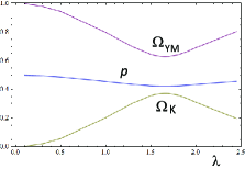
(b)

Figure 15: The averaged values of $\Delta_{0}$ (a), the power exponent of the scale factor $p$ and density parameters ($\Omega_{\scriptscriptstyle{\rm YM}},\Omega_{V}$ and $\Omega_{K}$) (b) for $\alpha=4$ and $\lambda>0$.

VI Concluding Remarks

We have studied an SU(2) non-Abelian gauge field coupled exponentially to a scalar field with an exponential potential, while making a comparison with the U(1) multiplet case.

We found that the power-law inflation with the magnetic component of the gauge field ($B_{\scriptscriptstyle{\rm YM}}$-I) is possible and it is an attractor of the present system, if $\lambda>\alpha$ and $\lambda>-\alpha+4/\alpha$. The transfer of scalar kinetic energy to the gauge fields through the gauge-kinetic coupling makes an inflationary solution possible even for a steep potential such as $\alpha>\sqrt{2}$, which is expected in the unified theories of fundamental interactions.

On the other hand, the inflationary solution dominated by the electric component ($E_{\scriptscriptstyle{\rm YM}}$-I) turned out to be unstable in contrast to the U(1) multiplet case. It can be a transient if the initial conditions are tuned. The attractor of the system is instead the conventional power-law inflation ($S_{\scriptscriptstyle{\rm YM}}$-I) if $\alpha<\sqrt{2}$. The YM field with a small amplitude is oscillating in this background universe.

We have also found new fixed points ($NA_{\pm}$) in the parameter range of $\sqrt{6}<\lambda<\alpha$, which do not exist in the U(1) multiplet case. The fixed point $NA_{+}$ is an attractor, while $NA_{-}$ is unstable. We have also analyzed the non-inflationary regime, where the generic feature appears to be the oscillation of the YM fields ($O_{\pm}$).

We summarize our result in Fig. 16.

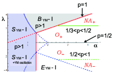
Figure 16: The phase diagram in the parameter space of the present model. An inflationary phase is the attractor in the shaded regions. Besides, an attractor solution of the conventional sense exists for $\lambda>\sqrt{6}$ ($NA_{+}$). For the rest of the space, the nature of the dynamics is oscillation of the YM field.

One may wonder whether those isotropic inflationary solutions are stable against anisotropic perturbations. Since there exist vector fields ($A_{\mu}^{\rm(a)}$), we usually find an anisotropic spacetime just as the case with a single U(1) gauge field. In order to prove the predictive power of the scenario, we have to show that the FLRW universe is obtained as an attractor in anisotropic Bianchi cosmologies. It is also interesting to know whether anisotropic inflation appears in a transient phase and its relic is observable or not. The study of Bianchi universe in the present model is in progress.

Another important subject in the present model is a graceful exit from a stable inflationary universe, including a reheating mechanism and a calculation of density fluctuations. In order to leave the power-law inflationary attractor that is a self-similar scaling solution, within the context of unified theories of fundamental interactions, we may have the following possibilities, which may also work for the U(1) triplet case:
(1) The moduli fixing: After a certain number of e-folds, if we can fix the moduli field $\phi$, the gauge-kinetic coupling vanishes. As a result, the inflation with magnetic component ($B_{\scriptscriptstyle{\rm YM}}$-I) will end.
(2) Hybrid-type Inflation: If $V_{0}$ is not just a constant but depends on another scalar field $\sigma$ as $V_{0}={m^{2}\over 2}\sigma^{2}$, we find a dynamics approximated by the present scenario for the large value of $\sigma$, and the end of inflation arrives when $\sigma$ gets small.
(3) Decay of the VEV of YM field: The YM field may be coupled to other particles. Through such a coupling, the particles can be created quantum mechanically, which will reduce the YM vacuum energy ($\rho_{\scriptscriptstyle{\rm YM}}$)Dimopoulos . The inflation assisted by YM field will eventually end.

As for the reheating of the universe, for the cases (1) and (2), since we have a potential minimum around which a scalar field will oscillate, we then find the reheating of the universe. It is not clear whether we can find the hot Big Bang state via the particle production assumed in the case (3).

The density fluctuations have been calculated for the case of U(1) triplet, which shows the leading order effect of the background gauge fields is consistent with the current observational dataYamamoto2 . While YM field is expected to give qualitatively similar results at the linear order, there is an interesting prospect of generating non-Gaussianity through the famous chaotic behaviors that are peculiar to the non-Abelian gauge fieldsYMchaos ; Jin ; Murata . These subjects are to be investigated in future works.

Appendix A Oscillation of the Yang-Mills field in the expanding universe

In some numerical calculations, we have seen the YM field oscillates very rapidly while the background spacetime evolves smoothly. If the energy density of the YM field is much smaller than that of the scalar field, the YM field does not contribute to the evolution of the universe. Even for the case that the YM field energy cannot be ignored, the oscillation of YM field may not directly affect the dynamics of the universe, but its mean value may contribute to the evolution of the universe. The different time-scales of the YM field oscillation and the evolution of FLRW universe may allow us to treat these two separately. Here we find such an oscillation of the YM field, assuming a given background spacetime and evolution of the scalar field.

Suppose the background is described by the following power-law solution:

$$a=a_{0}t^{p}\,,~{}~{}\phi=\varpi_{0}N+\phi_{0}\,,$$ (80)

where $p$ and $\varpi_{0}$ are constants, and $N=\ln(a/a_{0})$ is the e-folding time. The equation for the isotropic YM field in this background is given by

$$\ddot{A}+{p(1+\lambda\varpi_{0})\over t}\dot{A}+{2g_{\scriptscriptstyle{\rm YM}}^{2}\over a_{0}^{2}}{A^{3}\over t^{2p}}=0\,.$$ (81)

Changing the variables $t$ and $A$ to $\eta$ and $Z$, which are defined by

$$t = \left({\eta\over s}\right)^{s}\,,$$ (82)

$$A = {a_{0}g_{\scriptscriptstyle{\rm YM}}\over\sqrt{2}}\left({\eta\over s}\right)^{-\lambda p\varpi_{0}s/3}\,Z\,,$$ (83)

where

$$s={3\over 3-p(3+\lambda\varpi_{0})},\,$$ (84)

we find the following equation for $Z$:

$${d^{2}Z\over d\eta^{2}}-{\lambda p\varpi_{0}\over 9}\left[3(p-1)+2\lambda p\varpi_{0}\right]\left({\eta\over s}\right)^{2[3(p-1)+\lambda p\varpi_{0}]s/3}Z+Z^{3}=0\,.$$ (85)

Let us discuss the case where $\eta$ increases as $t$ increases, i.e., we assume that $s>0$, or equivalently, $3(p-1)+\lambda p\varpi_{0}<0$. Hence this term in Eq. (85) may drop as $\eta\rightarrow\infty$ ($t\rightarrow\infty$). Once we ignore the second linear term, we find a simple non-linear differential equation

$${d^{2}Z\over d\eta^{2}}+Z^{3}=0\,,$$ (86)

which solves as

$$Z=Z_{0}{\rm cn}\left(Z_{0}\eta;{1\over\sqrt{2}}\right)\,,$$ (87)

where ${\rm cn}(x;k)$ is the Jacobi’s elliptic function. Then the YM field is described in terms of the cosmic time $t$ as

$$A={a_{0}g_{\scriptscriptstyle{\rm YM}}Z_{0}\over\sqrt{2}}t^{-\lambda p\varpi_{0}/3}{\rm cn}\left(Z_{0}s\,t^{1/s},{1\over\sqrt{2}}\right)\,.$$ (88)

Using this solution, we can evaluate the asymptotic behavior of the density parameter and the difference between magnetic and electric components of the YM field as

$$\Omega_{\scriptscriptstyle{\rm YM}} \propto t^{2-p(4+\lambda\varpi_{0}/3)}$$ (89)

$$\Delta = 2{\rm cn}^{4}\left(Z_{0}\eta;{1\over\sqrt{2}}\right)-1\,.$$ (90)

Since the above approximate solution contains the parameter $s$ (84), which depends on the background solution, there are the following two cases: (1) The background is controlled only by the scalar field. The YM field is oscillating in the background, but its energy density is too small to affect the evolution of the universe. (2) The other case is that the averaged value of $\Delta_{0}$ as well as $\Omega_{\scriptscriptstyle{\rm YM}}$ give an important contribution onto the background. In that case, we need an iterative procedure to find the correct averaged value $\Delta_{0}$, as shown in the main body of the article.

Here we present the averaged value of $\Delta$ and the properties of the asymptotic spacetime in the case (1). The results for the case (2) are given in §. V.2.

For inflation driven by a scalar field, we have $p=2/\alpha^{2}$ and $\varpi_{0}=\alpha$. Then the condition $3(p-1)+\lambda p\varpi_{0}<0$ is

$$\lambda<{3(\alpha^{2}-2)\over 2\alpha}\,.$$ (91)

This is always satisfied in the range we consider. The average of $\Delta$ must be taken in terms of the cosmic time $t$. We show our numerical result in Fig. 17.

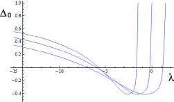
Figure 17: The averaged values of $\Delta_{0}$ for $\alpha=1,\sqrt{2}$ and $2$. It changes from $-0.4$ to $1$ depending on the value of $\lambda$.