Caloric curves fitted by polytropic distributions in the HMF model

Abstract

We perform direct numerical simulations of the Hamiltonian mean field (HMF) model starting from non-magnetized initial conditions with a velocity distribution that is (i) gaussian, (ii) semi-elliptical, and (iii) waterbag. Below a critical energy $E_{c}$, depending on the initial condition, this distribution is Vlasov dynamically unstable. The system undergoes a process of violent relaxation and quickly reaches a quasi-stationary state (QSS). We find that the distribution function of this QSS can be conveniently fitted by a polytrope with index (i) $n=2$, (ii) $n=1$, and (iii) $n=1/2$. Using the values of these indices, we are able to determine the physical caloric curve $T_{kin}(E)$ and explain the negative kinetic specific heat region $C_{kin}=dE/dT_{kin}<0$ observed in the numerical simulations. At low energies, we find that the system takes a “core-halo” structure. The core corresponds to the pure polytrope discussed above but it is now surrounded by a halo of particles. In case (iii), we recover the “uniform” core-halo structure previously found by Pakter & Levin [Phys. Rev. Lett. 106, 200603 (2011)]. We also consider unsteady initial conditions with magnetization $M_{0}=1$ and isotropic waterbag distribution and report the complex dynamics of the system creating phase space holes and dense filaments. We show that the kinetic caloric curve is approximately constant, corresponding to a polytrope with index $n_{0}\simeq 3.56$ (we also mention the presence of an unexpected hump). Finally, we consider the collisional evolution of an initially Vlasov stable distribution, and show that the time-evolving distribution function $f(v,t)$ can be fitted by a sequence of polytropic distributions with a time-dependent index $n(t)$ both in the non-magnetized and magnetized regimes. These numerical results show that polytropic distributions (also called Tsallis distributions) provide in many cases a good fit of the QSSs. They may even be the rule rather than the exception. However, in order to moderate our message, we also report a case where the Lynden-Bell theory (which assumes ergodicity or efficient mixing) provides an excellent prediction of an inhomogeneous QSS. We therefore conclude that both Lynden-Bell and Tsallis distributions may be useful to describe QSSs depending on the efficiency of mixing.

1 Introduction

Systems with long-range interactions are numerous in nature. They include, for example, self-gravitating systems and two-dimensional (2D) vortices which are systems of considerable interest houches . These systems may be trapped in long-lasting non-equilibrium states, called quasi-stationary states (QSS), whose lifetime diverges with the number of particles $N$. These QSSs correspond to galaxies in astrophysics and large-scale vortices (e.g. Jupiter’s great red spot) in 2D hydrodynamics. Therefore, in many cases of physical interest, the system does not reach the Boltzmann distribution but remains stuck in a non-Boltzmannian QSS. This is the case of elliptical galaxies in stellar dynamics because the collisional relaxation time exceeds the age of the universe by many orders of magnitude. This is also the case in 2D geophysical and astrophysical flows because the viscous time is generally much larger than the turnover time of a large-scale vortex. These QSSs are known to be stable steady states of the Vlasov (or 2D Euler) equation on a coarse-grained scale. The Vlasov equation describes the “collisionless” evolution of the system before “collisions” (more precisely correlations, finite $N$ effects, granularities…) drive the system towards Boltzmann’s statistical equilibrium. Since the Vlasov equation admits an infinite number of steady states, the prediction of the QSS that is actually selected by the system is difficult. Our understanding of these QSSs is still incomplete.

A toy model of systems with long-range interactions, called the Hamiltonian mean field (HMF) model, has been actively studied in statistical mechanics cdr . It consists of $N$ particles moving on a ring and interacting via a cosine potential. At statistical equilibrium, this system displays a second order phase transition between a spatially homogeneous (non-magnetized $M=0$) phase and a spatially inhomogeneous (magnetized $M\neq 0$) phase. The magnetized phase appears below the critical energy $E_{c}=3/4$ or below the critical temperature $T_{c}=1/2$. Antoni & Ruffo ar carried out direct numerical simulations of the HMF model. They started from an initial condition in which all the particles are located at $\theta=0$ (corresponding to a magnetization $M_{0}=1$) with a waterbag velocity distribution. They determined the physical caloric curve $T_{kin}(E)$ giving the average kinetic temperature as a function of the energy. They compared their numerical results to the theoretical caloric curve $T(E)$ corresponding to the Boltzmann equilibrium and reported several “anomalies”. In particular, the phase transition takes place at an energy sensibly smaller than $E_{c}=3/4$ and the numerical caloric curve $T_{kin}(E)$ presents a region of negative kinetic specific heats, unlike the theoretical caloric curve $T(E)$ corresponding to the Boltzmann equilibrium. They understood that these discrepancies are due to the fact that the observed structures are out-of-equilibrium QSSs. These results were confirmed by Latora et al. latora ; lrt who showed that the lifetime of these QSSs diverges with $N$ and that their distribution functions are non-Boltzmannian. They also observed many other anomalies in the region of negative kinetic specific heats such as anomalous diffusion, Lévy walks, aging, and dynamical correlations in phase-space. The observation of non-Boltzmannian QSSs was a surprise in the community of statistical mechanics. Latora et al. latora ; lrt proposed to interpret these QSSs in terms of Tsallis generalized thermodynamics tsallis . In particular, they tried to fit the QSS at $E=0.69$ by a $q$-distribution with a power-law tail. To make the distribution normalizable, they introduced a cut-off at large velocities. While their study definitely shows that the QSS is non-Boltzmannian, their procedure is not very convincing and their fit is relatively poor.

The situation changed after the conference in Les Houches in 2002 where it was indicated chavhouches that QSSs were previously observed in stellar dynamics and 2D turbulence. In these domains, the QSSs are interpreted in terms of Lynden-Bell’s statistical theory of violent relaxation lb . The Lynden-Bell theory determines the statistical equilibrium state of the Vlasov equation, taking into account all the constraints of the “collisionless” dynamics, in particular the conservation of the Casimirs. If the system is ergodic, the QSS coincides with the Lynden-Bell distribution (most probable state). In the two-levels case $(f_{0},0)$, the distribution predicted by Lynden-Bell is similar to the Fermi-Dirac distribution in quantum mechanics. When applied to the HMF model, the Lynden-Bell theory predicts an out-of-equilibrium phase transition between a magnetized and a non-magnetized phase, and a phenomenon of phase re-entrance in the $(f_{0},E)$ plane epjb . The nature of these phase transitions has been studied in detail in prl2 ; marseille ; staniscia1 ; staniscia2 . In particular, there exist a tricritical point separating first and second order phase transitions, and a critical point (associated with the re-entrant phase) marking the onset of a second order azeotropy staniscia2 . Direct numerical simulations staniscia1 ; precommun ; prl1 ; bachelard1 ; bachelard2 showed a good agreement with the Lynden-Bell prediction in certain cases but also evidenced discrepancies in other cases. For example, in staniscia1 , the re-entrant phase predicted from the Lynden-Bell theory in a very small range of parameters is confirmed (which is a success of the theory), but a secondary re-entrant phase that is not predicted by the Lynden-Bell theory is also observed (this secondary re-entrant phase has been recently confirmed by another group oy suggesting that it is not a numerical artifact). More generally, the adequacy, or inadequacy, of the Lynden-Bell theory to predict the magnetization of the QSS can be read from the numerical phase diagrams plotted in staniscia1 ; bachelard2 .

These discrepancies can be interpreted as a result of incomplete relaxation lb ; epjb ; incomplete ; hb3 ; hb4 . Indeed, the Lynden-Bell statistical theory is based on an assumption of ergodicity or, at least, efficient mixing. If the system does not mix well, the Lynden-Bell prediction fails and the system may be trapped in a steady state of the Vlasov equation that is not the most mixed state. This is precisely what happens in the case $M_{0}=1$ considered by Antoni & Ruffo ar and Latora et al. latora ; lrt . As discussed in epjb ; hb3 , the failure of the Lynden-Bell prediction is particularly clear in that case. Indeed, for an initial condition with $M_{0}=1$, we are in the non-degenerate (dilute) limit of the Lynden-Bell theory. In this limit, the Lynden-Bell distribution reduces to the Boltzmann distribution (with a different interpretation). Therefore, as argued in hb3 , the theoretical Boltzmann caloric curve plotted by Antoni & Ruffo ar and Latora et al. latora ; lrt should be interpreted as the theoretical Lynden-Bell caloric curve. Consequently, the observed discrepancies between this theoretical caloric curve and the numerical results reveal the failure of the Lynden-Bell prediction in that case (this is confirmed by the phase diagrams of staniscia1 ; bachelard2 ). Therefore, the Lynden-Bell theory does not explain everything. The limitations of the Lynden-Bell theory were emphasized in epjb ; incomplete .

Following these observations, it has been proposed cc ; epjb ; cstsallis that Tsallis $q$-distributions may provide a good fit of the QSSs in certain cases of incomplete relaxation. At the same time, it has been emphasized that this good agreement is not expected to be general, i.e. the Tsallis distributions are not universal attractors. Actually, $q$-distributions correspond to what have been called stellar polytropes in astrophysics bt . They were introduced long ago by Eddington eddington as particular stationary solutions of the Vlasov equation. They were used to construct simple self-consistent mathematical models of galaxies. At some time, they were found to provide a reasonable fit of some observed star clusters, the so-called Plummer plummer model. Improved observation of globular clusters and galaxies showed that the fit is not perfect and more realistic models have been introduced since then bt . However, stellar polytropes are still important in astrophysics for historical reasons and for their mathematical simplicity. Similarly, we believe that these distributions will play a useful role in the HMF model. Of course, the relevance (or irrelevance) of $q$-distributions can only be assessed by the results of numerical simulations that we now briefly review.

Campa et al. campa1 performed direct numerical simulations of the HMF model starting from an initial condition with magnetization $M_{0}=1$ and a waterbag velocity distribution corresponding to an energy $E=0.69$. They obtained a non-magnetized QSS with a velocity distribution that they called “semi-ellipse”. Chavanis hb3 noted that this distribution is a particular polytropic (Tsallis) distribution with index $n=1$. This was the first clear evidence of a polytropic QSS in the HMF model. Furthermore, this distribution has a compact support which is very natural in the phenomenology of incomplete violent relaxation. Chavanis & Campa cc developed a general theory of polytropic distributions in the context of the HMF model. In this approach, polytropic distributions are interpreted as particular steady states of the Vlasov equation, like in astrophysics bt . They studied the dynamical stability problem by using a “thermodynamical analogy” and evidenced a rich variety of phase transitions depending on the polytropic index $n$ (or $q$). They computed the physical caloric curves $T_{kin}(E)$ and found that, for $0.54<n<3.56$, these curves display a region of negative kinetic specific heat $C_{kin}<0$ (see in particular Figure 23 of cc ). They proposed that these results could help interpreting the “anomalies” reported by Antoni & Ruffo ar that have never been explained so far.

Pakter & Levin levin performed direct numerical simulations of the HMF model starting from a rectangular waterbag distribution with $M_{0}=0.40$ and different values of the energy. They found that the QSS has a core-halo structure. The core corresponds to a completely degenerate distribution in the Lynden-Bell theory (i.e. the ground state at $T=0$). The halo is interpreted in terms of a parametric resonance. This core-halo structure is not consistent with the Lynden-Bell prediction that leads to a partially degenerate distribution without core-halo structure. In addition, for $M_{0}=0.40$, the Lynden-Bell theory predicts a second order phase transition prl2 while Pakter & Levin levin find a first order phase transition. We note that the homogeneous core, interpreted as a completely degenerate Lynden-Bell distribution, is a polytrope $n=1/2$ (waterbag distribution) hmfq1 . Therefore, the first order phase transition reported by Pakter & Levin levin may be connected to the first order phase transition found by Chavanis hmfq1 for the pure waterbag distribution (compare Figure 6 of hmfq1 to Figure 2 of levin ).

Morita & Kaneko mk performed direct numerical simulations of the HMF model starting from initial conditions in which the angles and the velocities of the particles have Boltzmannian distributions with different temperatures. They found initial conditions for which the system does not relax toward a QSS. In their simulations, the magnetization exhibits persistent oscillations whose duration diverges with $N$. This long-lasting periodic or quasi periodic collective motion appears through Hopf bifurcation and is due to the presence of clumps (high density regions) in phase space.

This brief review of numerical results in the HMF model shows that the nature of the QSS crucially depends on the initial condition. The purpose of this paper is to investigate other initial conditions that have not been studied previously. We first consider non-magnetized initial states with a velocity distribution that is (i) gaussian, (ii) semi-elliptical, and (iii) waterbag. In each case, we determine the physical caloric curve $T_{kin}(E)$ of the corresponding QSS and plot the distribution function $f(\theta,v)$ as a function of the individual energy $\epsilon=v^{2}/2+\Phi(\theta)$. A steady state of the Vlasov equation is characterized by a function $f=f(\epsilon)$. In each case, we find that the caloric curve presents a region of negative kinetic specific heat: $C_{kin}=dE/dT_{kin}<0$. In that region, we find that the QSS is described by a distribution function $f=f(\epsilon)$ that can be conveniently fitted by a pure polytrope with index (i) $n=2$, (ii) $n=1$, and (iii) $n=1/2$. Using the values of these indices, we are able to determine the theoretical caloric curve $T_{kin}(E)$ and explain the negative kinetic specific heat region found in the numerical simulations. For lower energies, we find that the system takes a “core-halo” structure. The core corresponds to the pure polytrope discussed above but it is now surrounded by a halo of particles. In case (iii), the distribution function in the core is constant ($n=1/2$ polytrope) and we recover the results of Pakter & Levin levin . We also investigate the time evolution of the magnetization in the timescale corresponding to the QSS. We find persistent oscillations similar to those reported by Morita & Kaneko mk . In cases (i) and (ii), they are slowly damped, and in case (iii) they are more persistent. We interpret these oscillations in relation to the Landau damping around a spatially inhomogeneous QSS. For the spatially homogeneous waterbag distribution, we know that there is no Landau damping. By continuity, the damping rate should be small in the inhomogeneous case, and this may explain the numerical results. We also consider unsteady initial conditions with $M_{0}=1$ and isotropic waterbag velocity distribution. In that case, we find that the system forms phase space holes and dense filaments that persist for a very long time. Ultimately, these holes disappear and a QSS is formed. We show that the kinetic caloric curve is approximately constant, corresponding to a polytrope with index $n_{0}\simeq 3.56$. This sensibly differs from the results reported in ar ; latora . Finally, we consider the collisional evolution of an initially Vlasov stable distribution, and show that the time-evolving distribution function $f(v,t)$ can be fitted by a sequence of polytropic distributions with a time-dependent index $n(t)$ both in the non-magnetized and magnetized regimes.

Before discussing these numerical results (Sections 4-6), we summarize our theory of polytropes cc , and provide additional theoretical results that were not given in our previous paper (Section 3). In particular, we analyze in more detail the nature of the kinetic caloric curve $T_{kin}(E)$ as a function of the polytropic index $n$ since these curves are of considerable importance to interpret the numerical simulations. Some readers may skip this theoretical part and go directly to Section 4 where the results of numerical simulations are presented.

2 The HMF model

2.1 The Hamiltonian equations

The HMF model can be viewed as a collection of $N$ particles of unit mass moving on a circle and interacting via a cosine binary potential cdr . The dynamics of these particles is governed by the Hamilton equations

$$\frac{d\theta_{i}}{dt}=\frac{\partial H}{\partial v_{i}},\qquad\frac{dv_{i}}{dt}=-\frac{\partial H}{\partial\theta_{i}},\qquad$$ (1)

$$H=\frac{1}{2}\sum_{i=1}^{N}v_{i}^{2}+\frac{1}{2N}\sum_{i,j=1}^{N}[1-\cos(\theta_{i}-\theta_{j})],$$ (2)

where $\theta_{i}\in[0,2\pi[$ is the angle that particle $i$ makes with an axis of reference $Ox$ and $v_{i}=d\theta_{i}/dt\in]-\infty,+\infty[$ is its velocity. The HMF model conserves the energy $H$ and the number of particles $N$. The order parameter is the magnetization ${\bf M}=(M_{x},M_{y})$ with components

$$M_{x}=\frac{1}{N}\sum_{i}\cos\theta_{i},\qquad M_{y}=\frac{1}{N}\sum_{i}\sin\theta_{i}.$$ (3)

The energy per particle $E=H/N$ can be written as

$$E=\frac{1}{2N}\sum_{i=1}^{N}v_{i}^{2}+\frac{1-M^{2}}{2},$$ (4)

where $M=(M_{x}^{2}+M_{y}^{2})^{1/2}$ is the modulus of the magnetization. The equations of motion (1) can be written in terms of the magnetization components $M_{x}$ and $M_{y}$ as

$$\frac{d\theta_{i}}{dt} = v_{i},$$ (5)

$$\frac{dv_{i}}{dt} = -M_{x}\sin\theta_{i}+M_{y}\cos\theta_{i}.$$ (6)

Following the Kac prescription kac , the interaction strength has been rescaled by a factor $1/N$. This is the right scaling to properly define the thermodynamic limit $N\rightarrow+\infty$ of a system with long-range interactions such as the HMF model. In this way, the total energy of the system $E\sim N$ is extensive. However, the energy remains fundamentally non-additive cdr .

The HMF model can be thought of as a set of $N$ globally coupled rotators or $XY$-spins ($\theta_{i}$ represents the orientation of the $i$-th rotator and $v_{i}$ is the conjugated momentum). In this respect, it is similar to the $XY$ model though the interaction is extended to all couples of spins instead of being restricted to nearest neighbors. It is also similar to a one dimensional periodic self-gravitating system where the potential of interaction has been truncated to the first Fourier mode.

2.2 The Liouville equation

We introduce the $N$-body distribution function $P_{N}(\theta_{1},v_{1},...,\theta_{N},v_{N},t)$ giving the probability density of finding, at time $t$, the first particle with position $\theta_{1}$ and velocity $v_{1}$, the second particle with position $\theta_{2}$ and velocity $v_{2}$ etc. It is normalized such that $\int P_{N}\prod_{i}d\theta_{i}dv_{i}=1$. For an isolated Hamiltonian system, such as the HMF model, the evolution of the $N$-body distribution function is governed by the Liouville equation

$${\partial P_{N}\over\partial t}+\sum_{i=1}^{N}\biggl{(}v_{i}{\partial P_{N}\over\partial\theta_{i}}+F_{i}{\partial P_{N}\over\partial v_{i}}\biggr{)}=0,$$ (7)

where $F_{i}=-{\partial U\over\partial\theta_{i}}=-\frac{1}{N}\sum_{j}\sin(\theta_{i}-\theta_{j})$ is the force acting on particle $i$ due to the interaction with the other particles. It can be written $F_{i}=-M_{x}\sin\theta_{i}+M_{y}\cos\theta_{i}$. The Liouville equation (7) contains exactly the same information as the $N$-body Hamiltonian system (1).

2.3 Collisionless evolution: The Vlasov equation

For systems with long-range interactions, it can be shown that the mean field approximation is exact at the thermodynamic limit $N\rightarrow+\infty$ bh . This means that the $N$-body distribution function is a product of $N$ one-body distributions

$$P_{N}(\theta_{1},v_{1},...,\theta_{N},v_{N},t)=\prod_{i}P_{1}(\theta_{i},v_{i},t).$$ (8)

Let us introduce the one-body distribution function $f(\theta,v,t)=\frac{1}{N}\langle\sum_{i=1}^{N}\delta(\theta-\theta_{i})\delta(v-v_{i})\rangle=P_{1}(\theta,v,t)$. It is normalized such that

$$I[f]\equiv\int f\,d\theta dv=1.$$ (9)

Substituting the decomposition (8) in the Liouville equation (7) and integrating over all variables except $\theta_{1}$, $v_{1}$, we find that, for a fixed interval of time $[0,T]$ (any) and $N\rightarrow+\infty$, the evolution of the distribution function $f(\theta,v,t)$ is governed by the Vlasov equation

$$\frac{\partial f}{\partial t}+v\frac{\partial f}{\partial\theta}-\frac{\partial\Phi}{\partial\theta}\frac{\partial f}{\partial v}=0,$$ (10)

where

$$\Phi(\theta,t)=\int_{0}^{2\pi}[1-\cos(\theta-\theta^{\prime})]\rho(\theta^{\prime},t)\,d\theta^{\prime},$$ (11)

is the self-consistent potential generated by the density of particles $\rho(\theta,t)=\int f(\theta,v,t)\,dv$. The density of particles is defined by $\rho(\theta,t)=\frac{1}{N}\langle\sum_{i=1}^{N}\delta(\theta-\theta_{i})\rangle=P_{1}(\theta,t)$ and it is normalized such that $\int\rho\,d\theta=1$. The mean force acting on a particle located at $\theta$ is $\langle F\rangle(\theta,t)=-\partial\Phi/\partial\theta=-\int_{0}^{2\pi}\sin(\theta-\theta^{\prime})\rho(\theta^{\prime},t)\,d\theta^{\prime}$. Expanding the cosine function in equation (11), we obtain

$$\Phi(\theta,t)=1-M_{x}(t)\cos\theta-M_{y}(t)\sin\theta,$$ (12)

where

$$M_{x}(t)=\int\rho(\theta,t)\cos\theta\,d\theta,$$ (13)

$$M_{y}(t)=\int\rho(\theta,t)\sin\theta\,d\theta,$$ (14)

are the components of the mean magnetization ${\bf M}(t)$. The mean force acting on a particle can be written $F(\theta,t)=-M_{x}(t)\sin\theta+M_{y}(t)\cos\theta$.

The Vlasov equation is a purely mean field equation ignoring collisions (more properly, correlations, graininess, finite $N$-effects…) between particles. It governs the collisionless evolution of the HMF model.

The Vlasov equation admits an infinite number of stationary solutions. Any spatially homogeneous distribution function $f=f(v)$ is a steady state of the Vlasov equation. On the other hand, spatially inhomogeneous distributions of the form $f=f(\epsilon)$, where $\epsilon=v^{2}/2+\Phi(\theta)$ is the individual energy, are also steady states of the Vlasov equation.

2.4 The mean field energy

In the mean field approximation, the energy of the system can be written as

$$E[f]=\int f\frac{v^{2}}{2}\,d\theta dv+\frac{1}{2}\int\rho\Phi\,d\theta=E_{kin}+W,$$ (15)

where $E_{kin}$ is the kinetic energy and $W$ the potential energy. Using equations (12)-(14), the potential energy can be expressed in terms of the magnetization as

$$W=\frac{1-M^{2}}{2}.$$ (16)

The average kinetic temperature $T_{kin}$ is defined by

$$E_{kin}=\frac{1}{2}T_{kin}.$$ (17)

Therefore, the energy can be rewritten

$$E=\frac{1}{2}T_{kin}+\frac{1-M^{2}}{2}.$$ (18)

For a fixed value of the energy, the kinetic temperature directly determines the magnetization, and vice versa. The local pressure is defined by

$$p(\theta,t)=\int fv^{2}\,dv.$$ (19)

The kinetic energy can therefore be written

$$E_{kin}=\frac{1}{2}\int p\,d\theta.$$ (20)

This expression will be useful in the following.

2.5 Incomplete violent relaxation

Starting from an unstable or unsteady initial condition, the Vlasov equation is expected to reach, on a coarse-grained scale, a QSS. This is called weak convergence in mathematics. This QSS is a stable steady state of the Vlasov equation. Since the Vlasov equation admits an infinity of steady states, the prediction of the QSS actually reached by the system is difficult. A prediction can be made based on Lynden-Bell’s statistical theory of violent relaxation. However, this theory assumes that the evolution of the system is ergodic, or at least that the mixing is efficient. There are cases where the Lynden-Bell theory gives a good prediction. However, there also exist cases where this prediction fails. In case of incomplete relaxation, the system can be stuck in a stable steady state of the Vlasov equation that is not the most mixed state, i.e. that differs from the Lynden-Bell distribution. In this paper, we consider a particular class of steady states of the Vlasov equation, called polytropic distributions, that may arise in case of incomplete relaxation. They are associated with the Tsallis “entropy” (in the sense given below).

3 Reminders and complements in the theory of polytropes

The theory of polytropes for the HMF model has been developed in cc . Since this theory is rather rich (several cases arise depending on the polytropic index) and not well-known, we provide here a summary of the main results. In complement to our previous paper, we (i) use more conventional notations, (ii) simplify some important formulae, (iii) treat a case that was forgotten, (iv) describe in detail the physical caloric curve $T_{kin}(E)$ that will be needed to interpret our numerical results, and (v) specifically consider the waterbag distribution which is a particular polytrope of index $n=1/2$.

3.1 Polytropic distributions in phase space

The Tsallis entropy is defined by

$$S[f]=-\frac{1}{q-1}\int(f^{q}-f)\,d\theta dv,$$ (21)

with $q>0$. For $q\rightarrow 1$, it reduces to the Boltzmann entropy

$$S[f]=-\int f\ln f\,d\theta dv.$$ (22)

We consider the microcanonical problem

$$\max_{f}\quad\{S[f]\quad|\quad E[f]=E,\quad I[f]=1\},$$ (23)

and the canonical problem

$$\min_{f}\quad\{F[f]=E[f]-TS[f]\quad|\quad I[f]=1\}.$$ (24)

As explained in cc ; ccstab , these optimization problems determine particular steady states of the Vlasov equation of the form $f=f(\epsilon)$ with $f^{\prime}(\epsilon)<0$ that are dynamically stable. In this dynamical interpretation, $S$ is a pseudo entropy, $F$ is a pseudo free energy, and $T>0$ is a pseudo thermodynamical temperature. By an abuse of language, and to simplify the terminology, we shall omit the prefix “pseudo” in the sequel. However, we must keep in mind that all the references to thermodynamics in our study are purely effective: we are dealing with dynamical stability, not thermodynamical stability. Nevertheless, it is convenient to develop a thermodynamical analogy and use a similar terminology.

We recall that canonical stability (criterion (24)) implies microcanonical stability (criterion (23)) but the converse is wrong in case of ensembles inequivalence ellis . Furthermore, we recall that the thermodynamic-looking optimization problems (23) and (24) provide just sufficient conditions of Vlasov dynamical stability. More refined dynamical stability criteria are discussed in ccstab .

The critical points of entropy at fixed energy and normalization are determined by the variational principle

$$\delta S-\beta\delta E-\alpha\delta I=0,$$ (25)

where $\beta=1/T$ and $\alpha$ are Lagrange multipliers ($T$ is the thermodynamical temperature and $\alpha$ the chemical potential). This yields the Tsallis $q$-distributions

$$f(\theta,v)=\left\{\mu-\frac{(q-1)\beta}{q}\left[\frac{v^{2}}{2}+\Phi(\theta)\right]\right\}_{+}^{1/(q-1)},$$ (26)

where $\mu=[1-(q-1)\alpha]/q$. The notation $[x]_{+}$ stands for $[x]_{+}=x$ if $x\geq 0$ and $[x]_{+}=0$ if $x\leq 0$. These distributions are also obtained as critical points of the free energy at fixed normalization, satisfying $\delta F+\alpha T\delta I=0$. In astrophysics, they are known as “polytropic distributions” bt . They are generally labeled by a polytropic index $n$ that is related to the parameter $q$ by the relation

$$n=\frac{1}{2}+\frac{1}{q-1}.$$ (27)

For $n=1/2$ ($q\rightarrow+\infty$), the polytropic distribution function (26) reduces to the waterbag, or Fermi, distribution (see Section 3.8). For $n\rightarrow+\infty$ ($q\rightarrow 1$), it reduces to the isothermal (Maxwell-Boltzmann) distribution

$$f(\theta,v)=A^{\prime}e^{-\beta\left[\frac{v^{2}}{2}+\Phi(\theta)\right]}.$$ (28)

We need to distinguish two cases depending on the sign of $q-1$. (i) For $q>1$ ($n\geq 1/2$), the distribution function can be written as

$$f=A(\epsilon_{m}-\epsilon)_{+}^{1\over q-1},$$ (29)

where we have set $A=[\beta(q-1)/q]^{1\over q-1}$ and $\epsilon_{m}=q\mu/[\beta(q-1)]$. Such distributions have a compact support in phase space since they vanish for $\epsilon\geq\epsilon_{m}$. At a given position $\theta$, the distribution function vanishes at $v=v_{m}(\theta)=\sqrt{2(\epsilon_{m}-\Phi(\theta))}$. For $n=1/2$, $\epsilon_{m}$ and $v_{m}(\theta)$ correspond to the Fermi energy and to the Fermi velocity, respectively. (ii) For $0<q<1$ ($n<-1/2$), the distribution function can be written as

$$f=\frac{A}{(\epsilon_{0}+\epsilon)^{1\over 1-q}},$$ (30)

where we have set $A=[\beta(1-q)/q]^{1\over q-1}$ and $\epsilon_{0}=q\mu/[\beta(1-q)]$. Such distributions are defined for all individual energies. At a given position $\theta$, the distribution function behaves, for large velocities, as $f\sim v^{-2/(1-q)}\sim v^{-(1-2n)}$. In the following, we shall only consider distribution functions for which the density and the pressure are finite. This implies $1/3<q<1$ ($n<-1$).

Polytropic distributions may arise as a result of incomplete relaxation. In that case, the system does not mix well enough to justify the establishment of the Lynden-Bell distribution which corresponds to the most mixed state. In general, incomplete relaxation manifests itself by the fact that mixing takes place only in a subdomain of phase space. This generally leads to distribution functions with a compact support (the distribution function vanishes above a certain energy $\epsilon_{m}$) while the distribution function predicted by Lynden-Bell remains strictly positive for all values of the energy (which is rather unphysical). Polytropes with index $n\geq 1/2$ have this property of confinement and this is why, in our opinion, they play an important role in case of incomplete relaxation. Therefore, in the following, we shall essentially consider the case $n\geq 1/2$.

3.2 Polytropic equation of state

To any distribution function of the form $f=f(\epsilon)$ with $f^{\prime}(\epsilon)<0$, we can associate a corresponding barotropic gas by defining the density $\rho=\int f\,dv=\rho(\Phi)$ and the pressure $p=\int fv^{2}\,dv=p(\Phi)$, and eliminating $\Phi(\theta)$ between these two expressions. This determines a barotropic equation of state $p=p(\rho)$. For the polytropic distribution (26), we get cc :

$$p=K\rho^{\gamma},\qquad\gamma=1+{1\over n},$$ (31)

with

$$K={1\over n+1}\biggl{\{}\sqrt{2}A{\Gamma(1/2)\Gamma(1/2+n)\over\Gamma(n+1)}\biggr{\}}^{-{1\over n}},$$ (32)

for $n\geq 1/2$ and

$$K=-{1\over n+1}\biggl{\{}\sqrt{2}A{\Gamma(-n)\Gamma(1/2)\over\Gamma(1/2-n)}\biggr{\}}^{-{1\over n}}.$$ (33)

for $n<-1$. Equation (31) is the well-known polytropic equation of state. This is the reason why the distributions (26) are called polytropic distributions. The polytropic constant $K$ is sometimes called the “polytropic temperature”. We can show that $K$ is a monotonically increasing function of the thermodynamical temperature $T$ cc . For isothermal systems ($q=1$, $n=\infty$, $\gamma=1$), we have $K=T$.

3.3 Polytropic distributions in physical space

The density is obtained by integrating Eq. (26) over the velocity. We find that the density is related to the potential $\Phi(\theta)$ by cc :

$$\rho(\theta)=\left[\lambda-\frac{\gamma-1}{K\gamma}\Phi(\theta)\right]_{+}^{\frac{1}{\gamma-1}},$$ (34)

where $\lambda=\epsilon_{m}/(K(n+1))$ for $n\geq 1/2$ and $\lambda=\epsilon_{0}/(-K(n+1))$ for $n<-1$. For $\gamma=1$, Eq. (34) reduces to the isothermal (Boltzmann) distribution

$$\rho(\theta)=Ae^{-\beta\Phi(\theta)},$$ (35)

with $A=(2\pi/\beta)^{1/2}A^{\prime}$. The polytropic distribution in physical space $\rho=\rho(\Phi)$ given by Eq. (34) has the same mathematical form as the polytropic distribution in phase space $f=f(\epsilon)$ given by Eq. (26) with $\gamma$ playing the role of $q$ and $K$ playing the role of $T=1/\beta$. In this correspondence, $\gamma$ is related to $q$ by Eqs. (27) and (31) leading to $\gamma=(3q-1)/(q+1)$ and $K$ is related to $T$ by Eqs. (32) and (33). Polytropic distributions (including the isothermal distribution) are apparently the only distributions for which $f(\epsilon)$ and $\rho(\Phi)$ have the same mathematical form.

Using Eq. (34), the polytropic distribution function (26) can be rewritten cc :

$$f(\theta,v)={1\over Z}\biggl{[}\rho({\theta})^{1/n}-{v^{2}/2\over(n+1)K}\biggr{]}_{+}^{n-1/2},$$ (36)

where $Z$ is given for $n\geq 1/2$ by

$$Z=\sqrt{2}{\Gamma(1/2)\Gamma(1/2+n)\over\Gamma(n+1)}[K(n+1)]^{1/2},$$ (37)

and for $n<-1$ by

$$Z=\sqrt{2}{\Gamma(-n)\Gamma(1/2)\over\Gamma(1/2-n)}[-K(n+1)]^{1/2}.$$ (38)

For $n\rightarrow+\infty$, we recover the isothermal distribution

$$f(\theta,v)=\left(\frac{\beta}{2\pi}\right)^{1/2}\rho(\theta)\,e^{-\beta\frac{v^{2}}{2}}.$$ (39)

Other useful expressions of the polytropic distribution function are given in cc .

3.4 Homogeneous phase: Jeans-type instability

It is convenient to define the polytropic temperature by

$$\Theta=K\left(\frac{1}{2\pi}\right)^{\gamma-1}.$$ (40)

In the homogeneous phase ($M=0$), using Eqs. (36) and (40), the polytropic (Tsallis) distributions can be written

$$f(v)=C\left[1-\frac{v^{2}}{2(n+1)\Theta}\right]_{+}^{n-1/2},$$ (41)

where $C$ is given for $n\geq 1/2$ by

$$C=\frac{1}{2\pi}\frac{\Gamma(n+1)}{\Gamma(1/2)\Gamma(1/2+n)}\frac{1}{\sqrt{2(n+1)\Theta}},$$ (42)

and for $n<-1$ by

$$C=\frac{1}{2\pi}\frac{\Gamma(1/2-n)}{\Gamma(1/2)\Gamma(-n)}\frac{1}{\sqrt{-2(n+1)\Theta}}.$$ (43)

For $n\geq 1/2$, the maximum velocity is $v_{max}=\sqrt{2(n+1)\Theta}$. For $n\rightarrow+\infty$, Eq. (41) reduces to the isothermal (Maxwell) distribution

$$f(v)=\left(\frac{\beta}{2\pi}\right)^{1/2}\rho\,e^{-\beta\frac{v^{2}}{2}}.$$ (44)

On the other hand, using Eqs. (20), (31) and (40), we find that the energy can be written as

$$E=\frac{1}{2}\Theta+\frac{1}{2}.$$ (45)

Therefore, in the homogeneous phase, the kinetic temperature coincides with the polytropic temperature:

$$T_{kin}=\Theta.$$ (46)

In addition, the caloric curve $\Theta(E)$ is the same for all indices $n$. It is defined for $T_{kin}=\Theta\geq 0$ and $E\geq 1/2$. The specific heat is $C=dE/d\Theta=dE/dT_{kin}=1/2$. The equality (46) is not true anymore in the inhomogeneous phase.

For the polytropic equation of state (31), the square of the velocity of sound in the homogeneous phase is given by

$$c_{s}^{2}=K\gamma\rho^{\gamma-1}=\gamma\Theta.$$ (47)

It can be shown that a spatially homogeneous distribution function $f(v)$ with a single maximum at $v=0$ is dynamically stable if, and only, if

$$1+\pi\int_{-\infty}^{+\infty}{{f^{\prime}(v)}\over v}dv>0.$$ (48)

For a distribution function of the form $f=f(v^{2})$ with $f^{\prime}(v^{2})<0$, the stability criterion can also be written as

$$c_{s}^{2}>\frac{1}{2}.$$ (49)

These two stability criteria are equivalent and they determine the spectral, linear and formal stability of the distribution cvb ; ccstab ; yamaguchi ; cd . According to these stability criteria, the homogeneous phase of a polytropic distribution is stable if cvb ; cc :

$$\Theta>\Theta_{c}\equiv\frac{1}{2\gamma},\qquad E>E_{c}=\frac{1}{4\gamma}+\frac{1}{2},$$ (50)

and unstable otherwise. For isothermal distributions ($n=\infty$, $\gamma=1$, $q=1$), we recover the critical values $(T_{c},E_{c})=(1/2,3/4)$. For the waterbag distribution ($n=1/2$, $\gamma=3$, $q=+\infty$), we get $(\Theta_{c},E_{c})=(1/6,7/12)$. For the semi-ellipse ($n=1$, $\gamma=2$, $q=3$), we obtain $(\Theta_{c},E_{c})=(1/4,5/8)$. As shown in previous works ik ; inagaki ; cvb ; cd , the instability below $E_{c}$ is similar to the Jeans instability in astrophysics bt .

3.5 Inhomogeneous phase: complete and incomplete polytropes

We now consider spatially inhomogeneous polytropic distributions. We can assume without loss of generality that the distribution is symmetrical with respect to the $x$-axis (i.e. with respect to the angle $\theta=0$). In that case, the potential can be written $\Phi(\theta)=1-M\cos\theta$ where $M=\int_{0}^{2\pi}\rho(\theta)\cos\theta\,d\theta$ is the magnetization ($M_{y}=0$ and $M=M_{x}$). The density profile (34) can be rewritten cc :

$$\rho(\theta)=A\left(\kappa+\frac{x}{n+1}\cos\theta\right)_{+}^{n}.$$ (51)

where we have noted

$$x=\frac{M}{KA^{1/n}}.$$ (52)

We must consider two cases $\kappa=\pm 1$. As realized in hmfq1 , the case $\kappa=-1$ was forgotten in cc . However, this forgetfulness does not alter the study of phase transitions made in cc since the branch $\kappa=-1$ only completes the caloric curve up to the ground state $E=0$.

For $x>0$, the density profile is concentrated around $\theta=0$ and for $x<0$, we get a symmetrical density profile concentrated around $\theta=\pi$. We can therefore restrict ourselves to $x\geq 0$. For $x=0$, we recover the homogeneous distribution $\rho=1/(2\pi)$. For $x>0$, the density profile is monotonically decreasing. Let us first assume $n\geq 1/2$ (i.e. $1\leq\gamma\leq 3$) and $\kappa=+1$. If $x<x_{c}\equiv n+1=\gamma/(\gamma-1)$, the density is strictly positive on $-\pi\leq\theta\leq\pi$ (incomplete polytrope). If $x>x_{c}$, the density has a compact support (complete polytrope). In that case, it vanishes for $|\theta|\geq\theta_{c}=\arccos(-x_{c}/x)$. We note that $\theta_{c}\geq\pi/2$. For $x\rightarrow+\infty$, the density profile is given by $\rho(\theta)=\Gamma((2+n)/2)/[\sqrt{\pi}\Gamma((1+n)/2)]\cos^{n}\theta$ cc . We now assume $n\geq 1/2$ and $\kappa=-1$. The central density is defined only for $x>x_{c}$. In that case, the polytrope is complete: the density vanishes for $|\theta|\geq\theta_{c}=\arccos(x_{c}/x)$. We note that $\theta_{c}\leq\pi/2$. For $x\rightarrow x_{c}$, the distribution tends to a Dirac peak $\rho(\theta)=\delta(\theta)$. Finally, we consider the case $n<-1$ (i.e. $0\leq\gamma\leq 1$) and $\kappa=+1$. The central density is defined only for $x<x_{c}=|n+1|=|\gamma/(\gamma-1)|$ and the polytrope is incomplete. Some typical density profiles are represented below in Figures 18 and 19.

The amplitude $A$ of the density profile (51) is determined by the normalization condition $\int\rho\,d\theta=1$, leading to

$$A=\frac{1}{2\pi I_{\gamma,0}(x)}.$$ (53)

where we have introduced the $\gamma$-deformed modified Bessel functions cc :

$$I_{\gamma,m}(x)=\frac{1}{2\pi}\int_{-\pi}^{\pi}\left(\kappa+\frac{\gamma-1}{\gamma}x\cos\theta\right)_{+}^{\frac{1}{\gamma-1}}\cos(m\theta)\,d\theta.$$ (54)

On the other hand, substituting Eq. (51) in Eq. (13) for the magnetization, we obtain the self-consistency relation

$$M=\frac{I_{\gamma,1}(x)}{I_{\gamma,0}(x)}.$$ (55)

Combining Eqs. (52), (53) and (55), we find that the polytropic temperature (40) is given by

$${\Theta}=\frac{1}{x}\frac{I_{\gamma,1}(x)}{I_{\gamma,0}(x)^{2-\gamma}}.$$ (56)

Finally, after some calculations cc , we can show that the kinetic temperature and the energy are given by

$$T_{kin}=\frac{\gamma-1}{\gamma}M^{2}+\kappa\frac{M}{x}.$$ (57)

$$E=\frac{1}{2}T_{kin}+\frac{1-M^{2}}{2}.$$ (58)

Equation (57) is equivalent to equation (109) of cc after a straightforward simplification. From equations (55)-(58), we can obtain the curves $\Theta(E)$, $M(\Theta)$, $M(E)$, and $T_{kin}(E)$ in parametric form with parameter $x$. Some of these curves have been analyzed in detail in cc . This analysis will be completed in Section 3.6.

Close to the bifurcation point ($E_{c},\Theta_{c})$, i.e. for $x\rightarrow 0$, using the asymptotic expansions given in cc , we find that the thermodynamical specific heat $C={dE}/{d\Theta}$ is given by

$$C=-\frac{2\gamma^{2}-5\gamma-2}{2(2-\gamma)}.$$ (59)

Let us introduce the critical indices

$$\gamma_{*}=\frac{5+\sqrt{41}}{4}\simeq 2.8507811...$$ (60)

$$n_{*}=\frac{4}{1+\sqrt{41}}\simeq 0.54031242...$$ (61)

The specific heat of the inhomogeneous phase at the bifurcation point is positive for $n>1$, negative for $n_{*}<n<1$ and positive again for $1/2\leq n<n_{*}$. It is infinite for $n=1$ and vanishes for $n=n_{*}$. For $n<-1$, the specific heat is always positive. These results explain the behavior of the caloric curve $\Theta(E)$ close to the bifurcation point cc . For the waterbag distribution ($n=1/2$, $\gamma=3$, $q=+\infty$), we get $C=1/2$ like in the homogeneous phase hmfq1 . For the semi-ellipse ($n=1$, $\gamma=2$, $q=3$), we obtain $C=\infty$. On the other hand, close to the critical point, the magnetization is given as a function of the energy by

$$M^{2}=\frac{8\gamma}{2\gamma^{2}-5\gamma-2}(E-E_{c}).$$ (62)

For isothermal distribution ($n\rightarrow+\infty$), the density profile (51) takes the form

$$\rho(\theta)=\frac{1}{2\pi I_{0}(x)}e^{\beta M\cos\theta},$$ (63)

with $x={M}/{T}$. The self-consistency relation (55) reduces to

$$M=\frac{I_{1}(x)}{I_{0}(x)}.$$ (64)

Finally, the temperature (56) or (57) and the energy (58) become

$$T=T_{kin}=\frac{M}{x},$$ (65)

$$E=\frac{1}{2}T+\frac{1-M^{2}}{2}.$$ (66)

Close to the bifurcation point ($E_{c},T_{c})$=($1/2$, $3/4$), the specific heat is $C={dE}/{dT}=5/2$ and the magnetization is $M=\sqrt{8/5}(E_{c}-E)^{1/2}$. This returns the well-known results of the Boltzmann thermodynamical analysis (see, e.g., cvb ).

3.6 The physical caloric curve

In our previous paper cc , we have plotted the thermodynamical caloric curves giving the thermodynamical temperature $T$, or the polytropic temperature $\Theta$, as a function of the energy $E$. This is the correct way to determine the stability of the system in canonical and microcanonical ensembles and study phase transitions. However, the temperature that is directly accessible to the experiments or to the numerical simulations is the kinetic temperature $T_{kin}$. In general, $T_{kin}\neq T=1/\beta$ in a QSS. For comparison with the numerical results of Sections 4-6, it is useful to study the physical caloric curve $T_{kin}(E)$ as a function of the polytropic index $n$. This study has been only partly done in our previous paper (see Figures 6 and 23 of cc ) and it is here systematically continued.

Close to the bifurcation point ($E_{c},T_{kin}^{c})$, i.e. for $x\rightarrow 0$, using the asymptotic expansions given in cc , we find that the physical (or kinetic) specific heat $C_{kin}={dE}/{dT_{kin}}$ is given by

$$C_{kin}=\frac{2\gamma^{2}-5\gamma-2}{2(2\gamma^{2}-\gamma-2)}.$$ (67)

Let us introduce the critical indices

$$\gamma_{0}=\frac{1+\sqrt{17}}{4}\simeq 1.2807764...$$ (68)

$$n_{0}=\frac{4}{\sqrt{17}-3}\simeq 3.5615528...$$ (69)

The kinetic specific heat of the inhomogeneous phase at the bifurcation point is positive for $n>n_{0}$, negative for $n_{*}<n<n_{0}$ and positive again for $1/2\leq n<n_{*}$. It is infinite for $n=n_{0}$ and vanishes for $n=n_{*}$. For $n<-1$, the kinetic specific heat is always positive. These results explain the behavior of the physical caloric curve $T_{kin}(E)$ close to the bifurcation point (see Figure 1). We note that for $1<n<n_{0}$, the solutions close to the bifurcation point have negative kinetic specific heat $C_{kin}=dE/dT_{kin}<0$ although they have positive thermodynamical specific heat $C=dE/dT>0$ cc . Therefore, one may observe negative kinetic specific heats although the ensembles are equivalent. A similar observation has been made in stfcn for the Lynden-Bell distribution.

Figure 1: The physical caloric curve for different values of $n$.

Figure 2: The physical caloric curve for $n>n_{0}$ (specifically $n=\infty$). The kinetic specific heat is positive. The physical caloric curve exhibits a second order phase transition at $E_{c}$.

Figure 3: The physical caloric curve for $n=n_{0}\simeq 3.56$. The kinetic specific heat close to the bifurcation point is infinite.

Figure 4: The physical caloric curve for $n_{MCP}\simeq 0.68<n<n_{0}$ (specifically $n=1.5$). The kinetic specific heat close to the bifurcation point is negative although the thermodynamical specific heat is positive cc .

Figure 5: The physical caloric curve for $n=1$. The kinetic specific heat close to the bifurcation point is negative ($C_{kin}=-1/2$). For $9/16\leq E\leq E_{c}=5/8$, the physical caloric curve is a straight line given by $T_{kin}=3/2-2E$. The thermodynamical specific heat is infinite cc .

Figure 6: The magnetization curve for $n>n_{MCP}$ (specifically $n=1$). For $9/16\leq E\leq E_{c}=5/8$, we have $M=2(E_{c}-E)^{1/2}$.

Figure 7: Microcanonical phase diagram for $n>n_{MCP}\simeq 0.68$. It shows a second order phase transition at $E_{c}$ and a region of negative kinetic specific heat between $E^{\prime}$ and $E_{c}$ for $n_{MCP}<n<n_{0}$.

Figure 8: Evolution of $T_{kin}^{c}$ and $T_{kin}^{*}$ as a function of $n$.

We must be careful that we cannot deduce any stability result in the canonical ensemble (the optimization problem (24)) from the physical caloric curve $T_{kin}(E)$ since $T_{kin}$ is not the correct variable (the correct variable in the canonical ensemble is $T$ or $\Theta$ cc ). Therefore, we restrict ourselves to the microcanonical ensemble (the optimization problem (23)). Actually, this is the most appropriate ensemble since the natural control parameter is the energy. Since phase transitions for polytropic distributions have already been discussed in our previous paper (from the thermodynamical caloric curve $\Theta(E)$), our discussion here will be more concise. We shall denote global entropy maxima by (S), local entropy maxima by (M) and minima or saddle points of entropy by (U). In the thermodynamical analogy, these symbols correspond to stable, metastable and unstable states. Coming back to the dynamical interpretation, stable states (S) and metastable states (M) are dynamically Vlasov stable. We cannot definitely conclude that unstable states (U) are Vlasov unstable, except for homogeneous distributions, since the optimization problem (23) provides just a sufficient condition of dynamical stability ccstab .

Figure 9: The physical caloric curve for $n_{MTP}\simeq 0.563<n<n_{MCP}$ (specifically $n=0.6$).

Figure 10: Enlargement of the physical caloric curve for $n_{MTP}<n<n_{MCP}$ (specifically $n=0.6$). The kinetic specific heat close to the bifurcation point is negative. The kinetic caloric curve displays a second order phase transition at $E_{c}$ and a first order phase transition at $E_{t}$. The transition energy $E_{t}$ has been determined from the entropy curve $S(E)$ as explained in cc . Note that the Maxwell construction cannot be performed on the physical caloric curve $T_{kin}(E)$ since $T_{kin}\neq T=1/\beta$.

Figure 11: The magnetization curve for $n_{MTP}<n<n_{MCP}$ (specifically $n=0.6$).

Figure 12: The physical caloric curve for $n_{*}<n<n_{MTP}$ (specifically $n=0.55$). The kinetic specific heat close to the bifurcation point is negative. There is a first order phase transition at $E=E_{t}$. The metastable branch exhibits a second order phase transition at $E_{c}$.

Figure 13: The magnetization curve for $n_{*}<n<n_{MTP}$ (specifically $n=0.55$).

Figure 14: The physical caloric curve for $n=n_{*}\simeq 0.54$. The kinetic specific heat close to the bifurcation point vanishes.

Figure 15: The physical caloric curve for $1/2\leq n<n_{*}$ (specifically $n=0.5$). The kinetic specific heat close to the bifurcation point is positive. There is just a first order phase transition.

Figure 16: The magnetization curve for $1/2\leq n<n_{*}$ (specifically $n=0.5$).

Figure 17: Microcanonical phase diagram.

For $n>n_{MCP}\simeq 0.68$, the physical caloric curve $T_{kin}(E)$ exhibits a second order phase transition marked by the discontinuity of $dT_{kin}/dE$ at $E=E_{c}$ (see Figures 2, 3, 4, and 5). An example of magnetization curve is given in Figure 6. For $n>n_{0}\simeq 3.56$, the kinetic specific heat is positive (see Figure 2). For $n_{MCP}<n<n_{0}$, there is a region of negative kinetic specific heat between $E^{\prime}$ and $E_{c}$ (see Figures 4 and 5). The microcanonical phase diagram in the $(n,E)$ plane for $n>n_{MCP}$ is represented in Figure 7. For completeness, we have also plotted $T_{kin}^{c}$ and $T_{kin}^{*}$ (the latter being the kinetic temperature corresponding to $E^{\prime}$) as a function of $n$ in Figure 8, although $T_{kin}$ should not be regarded as a control parameter. For $n_{MTP}\simeq 0.563<n<n_{MCP}$, there is a very interesting situation, already noted in cc , in which the caloric curve exhibits a second order phase transition at $E_{c}$ between the homogeneous phase and the inhomogeneous phase (as before) and a first order phase transition at $E_{t}$ between two inhomogeneous phases (see Figures 9-11). The first order phase transition is marked by the discontinuity of $T_{kin}$ at $E=E_{t}$ and the existence of metastable branches. Therefore, $n_{MCP}\simeq 0.68$ and $E_{MCP}\simeq 0.5873$ is a microcanonical critical point marking the appearance of the first order phase transition. At $n=n_{MTP}$, the energies of the first and second order phase transitions coincide ($E_{t}=E_{c}$) and, for $1/2\leq n<n_{MTP}$, there is only a first order phase transition at $E=E_{t}$ between homogeneous and inhomogeneous states (see Figures 12, 13, 14, and 15). Therefore, $n_{MTP}\simeq 0.563$ and $E_{MTP}\simeq 0.5901$ is a microcanonical tricritical point separating first and second order phase transitions. For $n_{*}\simeq 0.54<n<n_{MTP}$, there remains a sort of second order phase transition at $E=E_{c}$ for the metastable states (see Figures 12 and 13). Between $E^{\prime}_{*}$ and $E_{c}$, the kinetic specific heat is negative. At $n=n_{*}$, the kinetic specific heat close to the critical point vanishes and the energies $E^{\prime}_{*}$ and $E_{c}$ coincide (see Figure 14). For $1/2\leq n<n_{*}$, the kinetic specific heat close to the critical point is positive and the “metastable” second order phase transition disappears (the inhomogeneous states close to the bifurcation point are unstable). In that case, there is only a first order phase transition (see Figures 15 and 16). The microcanonical phase diagram in the $(n,E)$ plane summarizing all these results is represented in Figure 17.

In conclusion, for $n>n_{MCP}$ we have second order phase transitions, for $n_{MTP}<n<n_{MCP}$ we have first and second order phase transitions, and for $1/2\leq n<n_{MTP}$ we have first order phase transitions.

Remark 1: As a corollary, we emphasize that for $n>n_{MCP}\simeq 0.68$, the inhomogeneous polytropes are always entropy maxima at fixed energy and normalization so they are dynamically Vlasov stable. This is an important theoretical result of cc .

3.7 The polytrope $n=1$

The polytropic index $n=1$ (i.e. $\gamma=2$, $q=3$) is particular because it corresponds to a canonical tricritical point cc . Furthermore, for this index, the algebra greatly simplifies and analytical results can be obtained. This is because the relationship (34) between the density and the potential is linear.

The spatially homogeneous distribution is

$$f(v)=\frac{1}{2\pi^{2}\sqrt{\Theta}}\left(1-\frac{v^{2}}{4\Theta}\right)^{1/2},$$ (70)

if $|v|\leq v_{max}=2\sqrt{\Theta}$ and $f=0$ otherwise. It corresponds to what has been called “semi-ellipse” in campa1 . The homogeneous phase is dynamically stable if, and only, if $\Theta\geq\Theta_{c}=1/4$ or $E\geq E_{c}=5/8$.

The density profile of $n=1$ polytropes is

$$\rho(\theta)=A\left(\kappa+\frac{x}{2}\cos\theta\right)_{+}.$$ (71)

Some density profiles are plotted in Figure 18. For $\kappa=+1$ and $x<x_{c}=2$ (incomplete polytropes), the deformed Bessel functions take the simple form $I_{2,0}(x)=1$ and $I_{2,1}(x)={x}/{4}$. Then, we get

$$A=\frac{1}{2\pi},\quad\Theta=\frac{1}{4},\quad M=\frac{x}{4},$$ (72)

$$E=\frac{5}{8}-\frac{x^{2}}{64},\quad T_{kin}=\frac{1}{4}+\frac{x^{2}}{32}.$$ (73)

The spatially inhomogeneous distributions with $x<x_{c}$ have the same polytropic temperature $\Theta_{c}=1/4$ but different energies ranging from $9/16$ to $E_{c}=5/8$. Their magnetizations are in the range $0\leq M\leq 1/2$, and they are related to the energy by $M=2\sqrt{E_{c}-E}$ (see Figure 6). The thermodynamical caloric curve forms a plateau $\Theta(E)=\Theta_{c}$ in the range $9/16\leq E\leq 5/8$, so it has an infinite specific heat $C=dE/d\Theta=\infty$ (see Figure 12 of cc ). By contrast, in the same range of energies, the physical caloric curve (see Figure 5) is given by

$$T_{kin}=\frac{3}{2}-2E,$$ (74)

and it has a constant specific heat

$$C_{kin}=\frac{dE}{dT_{kin}}=-\frac{1}{2},$$ (75)

which turns out to be negative. Therefore, for $n=1$, the thermodynamical and physical caloric curves are very different.

Figure 18: Density profile of $n=1$ polytropes for different values of $x$. We have added the case $\kappa=-1$ that was forgotten in cc .

For complete polytropes, we can get analytical expressions of the thermodynamical parameters by using the following expressions of the $\gamma$-deformed modified Bessel functions:

$$I_{2,0}(x)=\frac{1}{2\pi}\left[\sqrt{x^{2}-4}+2\kappa\arccos\left(-\frac{2\kappa}{x}\right)\right],$$ (76)

$$I_{2,1}(x)=\frac{1}{2\pi}\left[\frac{\kappa}{x}\sqrt{x^{2}-4}+\frac{x}{2}\arccos\left(-\frac{2\kappa}{x}\right)\right].$$ (77)

Other analytical results are given in cc .

3.8 The waterbag distribution (polytrope $n=1/2$)

A detailed study of the possibly inhomogeneous waterbag distribution that is a steady state of the Vlasov equation has been performed in hmfq1 . Here, we only recall the main results of this study that will be needed to interpret the numerical simulations of Section 4.3. The waterbag distribution is defined by

$$f=\Biggl{\{}\begin{array}[]{cc}f_{0}&\qquad(\epsilon<\epsilon_{F}),\\ 0&\qquad(\epsilon\geq\epsilon_{F}).\end{array}$$ (80)

It is similar to the Fermi distribution in quantum mechanics where $f_{0}$ plays the role of the maximum value of the distribution function fixed by the Pauli exclusion principle and $\epsilon_{F}$ plays the role of the Fermi energy. Comparing Eq. (80) with Eq. (29), we see that the waterbag distribution corresponds to a polytrope of index $n=1/2$ (i.e. $\gamma=3$, $q=+\infty$). This correspondence can also be obtained by determining the equation of state associated with the waterbag distribution. To that purpose, we rewrite Eq. (80) in the form

$${f}=\Biggl{\{}\begin{array}[]{cc}f_{0}&\qquad(v<v_{F}(\theta)),\\ 0&\qquad(v\geq v_{F}(\theta)),\end{array}$$ (83)

where $v_{F}(\theta)=\sqrt{2(\epsilon_{F}-\Phi(\theta))}$ is the local maximum velocity (the analogous of the Fermi velocity in quantum mechanics). The density is given by $\rho(\theta)=2f_{0}v_{F}(\theta)$ and the pressure by $p(\theta)=(2/3)f_{0}v_{F}^{3}(\theta)$. Eliminating $v_{F}(\theta)$ between these two expressions, we find that the equation of state of the waterbag distribution is

$$p=\frac{1}{12f_{0}^{2}}\rho^{3}.$$ (84)

This is the equation of state of a polytrope of index $n=1/2$ and polytropic constant $K=1/(12f_{0}^{2})$. Therefore, $f_{0}$ is related to the polytropic temperature $\Theta=K/(2\pi)^{2}$ by

$$f_{0}=\frac{1}{4\pi\sqrt{3\Theta}}.$$ (85)

The velocity of sound is given by

$$c_{s}(\theta)=\frac{1}{2f_{0}}\rho(\theta)=v_{F}(\theta),$$ (86)

and it coincides with the maximum local velocity (the Fermi velocity in quantum mechanics).

The spatially homogeneous waterbag distribution is the step function

$$f=f_{0},\quad{\rm if}\quad|v|\leq v_{F},$$

$$f=0,\quad{\rm if}\quad|v|>v_{F},$$ (87)

where $v_{F}$ is determined by the normalization condition (9) leading to

$$v_{F}=\frac{1}{4\pi f_{0}}=\sqrt{3\Theta}.$$ (88)

The kinetic temperature is given by $T_{kin}=\Theta=v_{F}^{2}/3$, so the total energy can be written as

$$E=\frac{1}{6}v_{F}^{2}+\frac{1}{2}.$$ (89)

The velocity of sound in the homogeneous phase is $c_{s}=v_{F}$. According to the general criteria (48) and (49), the homogeneous phase is dynamically stable if

$$E>E_{c}=\frac{7}{12},\qquad\Theta>\Theta_{c}=\frac{1}{6},$$ (90)

$$f_{0}<(f_{0})_{c}=\frac{1}{2\pi\sqrt{2}},\qquad v_{F}>(v_{F})_{c}=\frac{1}{\sqrt{2}},$$ (91)

and unstable otherwise. These stability criteria can also be directly obtained from the dispersion relation $\epsilon(\omega)=0$ which can be solved analytically for the waterbag distribution (see, e.g., cvb ).

Figure 19: Density profile of $n=1/2$ polytropes for different values of $x$. For $\kappa=+1$ we have taken $x=1$ and $x=3$. For $\kappa=-1$ we have taken $x=3$.

Figure 20: Phase space portrait of $n=1/2$ incomplete ($x=1$) polytropes with $\kappa=+1$. The distribution function has the uniform value $f=\eta_{0}$ in the shaded area ($\epsilon<\epsilon_{F}$) and $f=0$ outside ($\epsilon>\epsilon_{F}$).

Figure 21: Phase space portrait of $n=1/2$ complete ($x=3$) polytropes with $\kappa=+1$. The distribution function has the uniform value $f=\eta_{0}$ in the shaded area ($\epsilon<\epsilon_{F}$) and $f=0$ outside ($\epsilon>\epsilon_{F}$).

Using the results of Section 3.5, the density profile of the spatially inhomogeneous waterbag distribution is given by

$$\rho(\theta)=\frac{1}{2\pi I_{3,0}(x)}\left(\kappa+\frac{2}{3}x\cos\theta\right)_{+}^{1/2},$$ (92)

with $\kappa={\rm sgn}(\epsilon_{F}-1)$. The polytrope is incomplete for $\kappa=+1$ and $x<x_{c}=3/2$, and complete otherwise. Some representative density profiles are plotted in Figure 19. The local maximum velocity is related to the local density by $v_{F}(\theta)=\rho(\theta)/(2f_{0})$, so it is proportional to the density profile. Combining Eqs. (56), (85), and (92), we obtain

$$v_{F}(\theta)=\sqrt{\frac{3I_{3,1}(x)}{xI_{3,0}(x)}}\left(\kappa+\frac{2}{3}x\cos\theta\right)_{+}^{1/2}.$$ (93)

The waterbag distribution is represented in phase space in Figures 20 and 21. The velocity distribution $\phi(v)$ can be obtained analytically hmfq1 .

The dynamical stability of the waterbag distribution has been studied in hmfq1 . The magnetization curve $M(E)$ is reproduced in Figure 16 and the physical caloric curve $T_{kin}(E)$ is plotted in Figure 15. There is a first order phase transition at $E_{t}=0.588$ marked by the discontinuity of the magnetization passing from $M_{t}=0.44$ to zero. The homogeneous phase is stable for $E>E_{t}$, metastable for $E_{c}=7/12<E<E_{t}$ and unstable for $0\leq E<E_{c}$. The inhomogeneous phase is stable for ($0\leq E<E_{t}$, $M_{t}<M\leq 1$), metastable for ($E_{t}<E\leq E_{*}=0.595$, $M_{*}=0.37\leq M<M_{t}$), and unstable for ($E_{c}<E<E_{*}$, $0<M<M_{*}$).

Remark 2: The magnetization curve $M(E)$ of the pure waterbag distribution (polytrope $n=1/2$) reported in Figure 16 (see also hmfq1 ) may be compared with Figure 2 of Pakter & Levin levin for a core-halo state in which the core is a polytrope $n=1/2$. They both exhibit a first order phase transition.

Remark 3: As discussed in hmfq1 , the waterbag distribution corresponds to the minimum energy state in the Lynden-Bell theory, when the initial condition has only two levels $0$ and $f_{0}$. This has been used to construct the curve $E_{ground}(f_{0})$ in Appendix A of staniscia2 .

4 Numerical simulations

We have performed a number of simulations of the HMF model that we analyze in this and in the following two Sections. We have considered different types of initial conditions. In this Section, we study the characteristics of the QSS that are reached by the system after a violent relaxation from a spatially homogeneous initial state which is Vlasov unstable. In Section 5, we study the evolution of the system initially prepared in a Vlasov stable spatially homogeneous state. In that case, the system is in a QSS from the beginning, and the slow evolution is due to finite size effects (“collisions”). We have already analyzed this evolution in the non-magnetized regime in Ref. campa2 , and here we extend our analysis to the magnetized regime. In Section 6, we treat the case in which the system is initially in an unsteady inhomogeneous state with magnetization $M_{0}=1$ and isotropic waterbag distribution.

In this Section, the initial distributions $f_{0}(v)$ of the velocities are of several types: Gaussian, i.e., $f_{0}(v)\propto{\rm e}^{-av^{2}}$, semi-elliptical, i.e., $f_{0}(v)\propto\sqrt{v_{0}^{2}-v^{2}}$, and waterbag, i.e., $f_{0}(v)\propto\theta(v_{m}-|v|)$, with the value of the parameters $a$, $v_{0}$ and $v_{m}$ determining the energy $E$. These three cases correspond to homogeneous polytropic distributions with $n=\infty$, $n=1$ and $n={1}/{2}$, respectively. In all cases, the energy $E$ is chosen smaller than the critical energy $E_{c}$ for Vlasov stability of the corresponding case. The critical energy, computed from Eq. (50), can be written in terms of $n$ as

$$E_{c}=\frac{3n+2}{4n+4}\,\,.$$ (94)

Substituting the values of $n$ we get that $E_{c}=0.75$ for the Gaussian distribution, $E_{c}={5}/{8}$ for the semi-elliptical distribution, and $E_{c}={7}/{12}$ for the waterbag distribution. The state is unstable if $E<E_{c}$. Then, after a rapid relaxation, the system settles down in a QSS. In this Section, our purpose is to analyze the physical caloric curves of the QSSs and to compare them with those of the polytropic distribution functions.

The simulations have been performed with $N=2^{17}$ particles. However, they are representative of a system with twice the number of particles, i.e., $2^{18}$, gaining in this way a factor of $2$ in the computer time needed. In fact, we have exploited the following symmetry property of the HMF model. If, in the initial conditions, for each particle with $(\theta,v)$ there is a particle with $(-\theta,-v)$, this property is conserved throughout the dynamics, keeping at the same time $M_{y}\equiv 0$. In fact, choosing the numbering of the particles in such a way that in the initial conditions we have $\theta_{i+\frac{N}{2}}=-\theta_{i}$ and $v_{i+\frac{N}{2}}=-v_{i}$, the equations of motion (5) give:

$$\frac{d^{2}\theta_{i+\frac{N}{2}}}{dt^{2}}=-M_{x}\sin\theta_{i+\frac{N}{2}}=M_{x}\sin\theta_{i}=-\frac{d^{2}\theta_{i}}{dt^{2}}\,\,,$$ (95)

that proves the statement. Furthermore, it is sufficient to follow (and thus to represent in the computer) the dynamics of only the first $\frac{N}{2}$ particles. We remark that extracting the initial condition from a distribution that is invariant under the inversion $(\theta,v)\to(-\theta,-v)$ should not introduce any peculiarity, since we expect that in the thermodynamic limit this invariance is satisfied.

We should note also the following point. The length of our simulations is sufficient to follow the rapid relaxation to the QSS and its initial stages. With $2^{18}$ particles the lifetime of the QSS is expected to be very large, since the collisional processes of the dynamics, due to finite size effects, are very slow. It is true that the lifetime of magnetized QSSs, as the ones we are going to analyze, is expected to be proportional to $N$ jstat , and not to a higher power of $N$ as for homogeneous QSSs campa1 ; however, such high values of $N$ lead to lifetimes that are much larger than the times we have considered. In conclusion, we have observed only the settling of the QSS in its inital form, before the slow collisional evolution has caused any significant variation in the direction of the BG equilibrium.

4.1 Gaussian initial conditions

In this case, for a given energy $E$, the initial velocities are extracted from the distribution

$$f_{0}(v)=\frac{1}{\sqrt{\pi\left(4E-2\right)}}\exp\left[-\frac{v^{2}}{4E-2}\right]\,\,.$$ (96)

The critical energy for Vlasov stability is $E_{c}=0.75$. We have performed simulations at several energies smaller than $E_{c}$, and precisely at the energy values $0.51$, $0.55$, $0.58$, $0.60$, $0.62$, $0.65$ and $0.69$. We note that the smallest possible energy for an initial condition with $M=0$ is $0.5$ (see Eq. (18)). In all cases, after the rapid relaxation, the system reaches a QSS with a magnetization smaller than the equilibrium value, and thus also with an average kinetic temperature smaller than at equilibrium (again from Eq. (18) one clearly sees that, for a given energy $E$, a decrease of $M$ implies a decrease of $T_{kin}$). In Figure 22 we show a representative plot of the magnetization vs time, $M(t)$, for the run at $E=0.58$.

Figure 22: Magnetization as a function of time $M(t)$ for $E=0.58$. It shows damped oscillations. They may be related to Landau damping for inhomogeneous QSS.

It appears that, after the rapid increase of $M$ and after a short transient with large oscillations, the system settles to a state with small persistent magnetization oscillations. The almost regularity of the oscillations indicates that they are not due to finite size noise, but that they are an intrinsic property of the QSS. Therefore, strictly speaking, we should consider the following two possibilities for the state reached by the system after the rapid relaxation. Either the state is not a stationary state of the Vlasov equation, but rather a quasi-periodic state; or the oscillations are due to a sort of Landau damping of an inhomogeneous QSS, and they will eventually die out on a time scale large with respect to the one simulated here. The first case is reminiscent of the results found by Morita and Kaneko mk , that studied initial conditions different from ours, and in some cases they obtained almost periodic oscillations of the magnetization.

A similar picture holds for the other energies studied, in some case with oscillations of a somewhat larger amplitude. Whatever the explanation of the oscillations, we can use the average value of the magnetization (and consequently the average value of the kinetic temperature) to characterize the state of the system; since the oscillations are small we can approximately consider the state to be stationary.

As already noted in the Introduction, a steady state (stable or unstable) of the Vlasov equation is characterized by a one particle distribution function that depends on $\theta$ and $v$ only through the individual energy $\epsilon=v^{2}/2+\Phi(\theta)$. Then, in our QSS the coordinates $(\theta,v)$ of the particles should be distributed according to this property. In our simulations, where $M_{y}\equiv 0$, the potential energy $\Phi(\theta)$ is given by $1-M_{x}\cos\theta$ (see Eq. (12)), where $M_{x}$ is the average value of the magnetization mentioned above. We have therefore divided the one particle phase space in cells small enough to characterize each cell with a good approximation with a single value of the individual energy $\epsilon$ (e.g., the value of the central point of the cell), but big enough to contain a large number of particles. Taking a snapshot of the system configuration in the QSS (at the end of the run), we have then counted the number of particles in each cell, and plotted this number vs the energy value attributed to the cells. If the points of this plot are arranged on a continuous line, this means that the one particle distribution function depends only on $\epsilon$, confirming that the state is a QSS.

In Figures 23 and 24 we plot the distribution $f(\epsilon)$ for the two cases $E=0.58$ and $E=0.55$, respectively. It is clear that, with a very good approximation, the points are arranged along a single line in both cases, confirming that the state of the system is a QSS. In particular, we note that the line is practically a straight line in Figure 23, while it is a straight line in Figure 24 up to a certain energy $\epsilon$, above which it deviates.

Figure 23: The distribution $f(\epsilon)$ has been fitted by a pure polytrope $n=3/2$ (long-dash) or $n=2$ (short-dash). We have also plotted the initial condition (dot).

Figure 24: The distribution $f(\epsilon)$ has been fitted by a polytropic core $n=3/2$ (long-dash) or $n=2$ (short-dash) and a halo. We have also plotted the initial condition (dot).

Looking at the polytropic distribution, Eq. (26), and at the relation between the indices $q$ and $n$ in Eq. (27), we see that an $f(\epsilon)$ given by a straight line between the minimum and maximum values of the individual energy, and zero for higher energies, corresponds to a polytrope with $n=3/2$. In Figure 24 and in Figure 23 the fit of the numerical distributions $f(\epsilon)$ with a straight line, i.e., with a polytrope with $n=3/2$, is reported. However, we report also the fit with a polytrope with index $n=2$, that, in spite of the different functional form, is numerically very close to the $n=3/2$ fit (it is actually slightly better). The use of the $n=2$ polytropes is in addition justified by the numerical caloric curve that we are going to discuss shortly.

From the operative point of view the fit is performed by writing Eq. (26) for $q>1$ in the following form:

$$f(\epsilon)=A(b-\epsilon)_{+}^{n-1/2}$$ (97)

with $n\geq{1}/{2}$. Once chosen, from the numerical distribution data, the minimum and maximum energies within which the fit has to be performed ($\epsilon_{min}$ and $\epsilon_{max}$ respectively), the parameter $b$ is equal to $\epsilon_{max}$, while $A(b-\epsilon_{min})_{+}^{n-1/2}$ is the value of the fit at the minimum energy.

The difference between $E=0.55$ and $E=0.58$ is evident: for $E=0.55$ the part of $f(\epsilon)$ at the higher energies $\epsilon$ is outside the fit. It is due to a halo of particles, and we have checked that this halo is robust and does not disappear at later times. Later, showing the results for the waterbag initial conditions, we will present a picture of the location of the particles in the one particle phase space in another case in which the halo in the distribution function $f(\epsilon)$ is evident.

The numerical distributions $f(\epsilon)$ for the other energies are not plotted here, and we briefly describe what has been obtained. For the smallest energy, $0.51$, and for the energies $0.60$ and $0.62$, the fit with $n={3}/{2}$ or $n=2$ is equally good, with the exception of the higher energies $\epsilon$ for $E=0.51$, where a halo is present as for $E=0.55$. For $E=0.62$ a small bending at the smaller and at the higher energies $\epsilon$ begins to appear in the numerical distribution, such that its second derivative is negative at small energies and positive at high enegies. This bending is marked at $E=0.65$ and even more pronounced at $E=0.69$. For these cases, the fit with a polytrope is not good, especially for $E=0.69$. This can easily be understood from Eq. (97): the sign of the second derivative of the polytrope is the same in all the energy range $[\epsilon_{min},\epsilon_{max}]$, i.e., positive for $n>{3}/{2}$ and negative for $n<{3}/{2}$.

In Figure 25 we plot, with white circles, the kinetic temperature as a function of the energy for the QSS reached by the system with gaussian initial conditions. Accordingly with the fit performed in Figures 23 and 24, we fit this numerical caloric curve with the analogous one that holds for $n={3}/{2}$ and $n=2$ polytropes (the fit by $n=2$ polytropes appears to be very good). Both of them show a negative kinetic specific heat in that energy range, and so does the numerical caloric curve. The explanation of this negative specific heat region in terms of polytropic, or close to polytropic distributions, is an important result of our paper. This is intrinsically due to incomplete relaxation (lack of ergodicity). We “guess” that the Lynden-Bell theory, which assumes complete mixing, would not produce a negative specific heat region.

Figure 25: The numerical caloric curve displays a region of negative kinetic specific heat $C_{kin}=dE/dT_{kin}<0$. It has been fitted by a polytrope $n=3/2$ for which $C_{kin}=-43/34$ and by a polytrope $n=2$ for which $C_{kin}=-5/2$.

We see that at the higher energies, $0.65$ and $0.69$, the fit of the caloric curve is less good, coherently with what has been found for the fit of the distribution functions. We note that at these energies the kinetic temperature of the QSS is not much higher than that of the homogeneous branch (equivalently, the magnetization of the QSS is small). It is then plausible that the relaxation from the homogeneous initial condition to the stable state can be approximately described by a quasi-linear theory, that treats the inhomogeneity of the distribution function as a perturbation of the angle-averaged homogeneous distribution. This is left for a future investigation quasilinear .

4.2 Semi-ellipse initial conditions

Now, for a given energy $E$, the initial velocities are extracted from the distribution

$$f_{0}(v)=\frac{1}{\pi\left(4E-2\right)}\sqrt{8E-4-v^{2}}\,\,,$$ (98)

corresponding to a $n=1$ homogeneous polytrope. The critical energy for Vlasov stability is $E_{c}={5}/{8}=0.625$. We have performed runs at the energies $0.51$, $0.55$, $0.58$, $0.59$, $0.60$ and $=0.61$. As before, after a rapid relaxation the system reaches a QSS with a magnetization and a kinetic temperature smaller than the respective equilibrium values.

We do not show analogous plots of the magnetization vs time, since they are very similar to those obtained for the gaussian initial conditions, with small persistent oscillations. We go directly to the plots of the numerical distribution functions. We show the two cases $E=0.59$ and $E=0.55$, respectively in Figures 26 and 27.

Figure 26: The distribution $f(\epsilon)$ has been fitted by a pure polytrope $n=1$ (dash). We have also plotted the initial condition (dot).

Figure 27: The distribution $f(\epsilon)$ has been fitted by a polytropic core $n=1$ (dash) and a halo. We have also plotted the initial condition (dot).

The points of the numerical distribution functions are arranged along a line, as it should be for a QSS. As for the gaussian case, the distributions at the smaller energies $E$ present a halo. The fit with a polytropic distribution has been performed with the $n=1$ polytrope. The fit appears rather good in both cases, of course except for the halo at $E=0.55$. The picture is similar as for the gaussian case, i.e., there is a halo at small energies (we have one also for $E=0.51$) and the fit with the polytrope worsen at high energies, here $E=0.60$ and $E=0.61$, when the sign of the second derivative of the numerical distributions is negative at small energies $\epsilon$ and positive at high energies. Actually, we found that also at energy $E=0.58$ the fit with a polytrope distribution is not satisfying.

In Figure 28 we show the numerical kinetic caloric curve of the QSS reached by the system, fitted by the $n=1$ polytropic kinetic caloric curve, that has a negative kinetic specific heat in that energy range. We see that the polytropic fit is relatively good for most energies. As for the gaussian case, at the highest energies the fit is less good, and probably the QSS in that case could be better explained by a perturbative analysis.

Figure 28: The numerical caloric curve displays a region of negative kinetic specific heat $C_{kin}=dE/dT_{kin}<0$. It has been fitted by a polytrope $n=1$ for which $C_{kin}=-1/2$.

We remark that the polytropic index that fits the QSS is the same as that of the initial velocity distribution, i.e. $n=1$.

4.3 Waterbag initial conditions

For this class of initial conditions, the initial velocities at a given $E$ are extracted from the distribution

$$f_{0}(v)=\frac{1}{2\sqrt{6E-3}}\Theta\left(\sqrt{6E-3}-|v|\right)\,\,,$$ (99)

corresponding to a $n={1}/{2}$ polytrope. The critical energy for Vlasov stability is $E_{c}={7}/{12}$. We have performed runs at the energies $0.51$, $0.55$, and $0.582$. The last energies is only very slightly smaller than the critical energy. While sharing the previous general picture, i.e., the rapid approach to a magnetized QSS, there are some new features. We begin by showng the plots of the magnetization vs time for the two energies $E=0.582$ and $E=0.55$, respectively in Figures 29 and 30.

Figure 29: Magnetization as a function of time $M(t)$ for $E=0.582$. It shows undamped (or slowly damped) oscillations. This may be related to the absence of Landau damping for the QSS ($=$ inhomogeneous waterbag) as for the homogeneous waterbag distribution.

Figure 30: Magnetization as a function of time $M(t)$ for $E=0.55$. The amplitude of the oscillations is smaller than in Figure 29. This may be due to the presence of the halo.

We note that the magnetization oscillations are more marked than previously, becoming very pronounced at $E=0.582$. This is relatively close to the situation reported by Morita & Kaneko mk . We noted before that one possible explanation of the oscillations is a Landau damping associated to the inhomogeneous QSS. Now, these large oscillations suggest that this damping could be very weak. It is suggestive to interpret this as a continuation with what happens for the homogeneous waterbag QSS, for which we know that Landau damping is absent (this being due to the singularity of the waterbag distribution, that, contrary to distributions strictly decreasing for increasing $|v|$, admits purely real proper frequencies).

Figure 31: The distribution $f(\epsilon)$ has been fitted by a “pure” homogeneous distribution (waterbag) corresponding to a $n=1/2$ polytrope. We have also plotted the initial homogeneous waterbag distribution (dot).

Figure 32: The distribution $f(\epsilon)$ has been fitted by a $n=1/2$ polytrope (core) with a halo. This “core-halo” structure is similar to the one found in levin . We have also plotted the initial homogeneous waterbag distribution (dot).

Nevertheless, we proceed as before and plot the numerical distributions as a function of the individual energy, using the average value of $M$ to define the last quantity. In Figures 31 and 32, we plot the numerical distributions for the cases $E=0.582$ and $E=0.55$, together with the fit with the $n={1}/{2}$ polytrope. At $E=0.582$, the QSS is an almost pure inhomogeneous waterbag distribution and the phase portrait looks like Fig. 21. At the smaller energy $E=0.55$ there is a halo that cannot be reproduced by the polytropic fit. This halo is clearly evident in Figure 33 that shows the location of all the particle in the one particle phase space in the QSS state at $E=0.55$. The boundary between the more densely populated region and the less densely populated region (the halo) is at the energy where the halo begins in Figure 32.

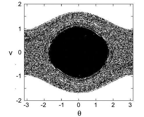
Figure 33: Occupation of the one particle phase space in the QSS state at $E=0.55$. The halo, i.e., the region less densely populated, is clearly visible.

Figure 34: Relation between the energy $E$ and the distribution value $f$ of a waterbag distribution that is a steady state of the Vlasov equation hmfq1 . Homogeneous and inhomogeneous distributions are represented. In the simulations, we start from an unstable homogeneous waterbag distribution with energy $E$ and distribution value $f_{0}$. We see that only at $E=E_{t}$ does the inhomogeneous polytrope have the same $f$ as the homogeneous polytrope. In the other cases, a halo is necessary to maintain the initial value $f_{0}$ in the core of the QSS (as observed in the simulations) while conserving energy. However, close to $E=E_{t}$, the effect of the halo is weak and a pure waterbag distribution provides a good approximation of the QSS.

As for the semi-ellipse initial conditions, we remark that the polytropic index of the QSS is the same as that of the initial velocity distribution, i.e. here $n=1/2$. A difference with respect to the two previous cases is that the fit appears to be good also very close to the critical energy $E_{c}$. Furthermore, the value of the numerical distribution function in the QSS is practically the same as that of the initial waterbag distribution (see Figures 31 and 32). This means that the core does not mix at all. Using this observation, we can explain the presence or the absence of the halo. To that purpose, we plot in Fig. 34 the relation between the uniform distribution value $f$ and the energy $E$ of a pure waterbag distribution that is solution of the Vlasov equation (the construction of this Figure is explained in hmfq1 ). This Figure shows the first order phase transition between homogeneous and inhomogeneous waterbag distributions discussed in Sec. 3.8. We see that, in general, the homogeneous and inhomogeneous waterbag distributions with the same $f$ have a different energy (see the vertical line in Fig. 34). Therefore, if $f$ is the same in the initial homogeneous waterbag distribution and in the inhomogeneous waterbag QSS (as it turns out to be), there must necessarily exist a halo of particles in order to satisfy the conservation of energy. The halo should be particularly important at low energies $E$ (as in Fig. 32 for $E=0.55$) where $\Delta E$ is large. By contrast, at the transition energy $E_{t}$, the homogeneous and inhomogeneous waterbag distributions have the same $f$ and $E$ so that the presence of a halo is not required. By continuity, close to the transition energy (as in Figure 31 for $E=0.582$), the halo should be modest since $\Delta E$ is small (for $E=0.582$ we find $\Delta E/E=0.01$). These arguments are consistent with the observations.

In Figure 35 we plot the numerical kinetic caloric curve, together with the $n={1}/{2}$ kinetic caloric curve. In principle, the $n={1}/{2}$ kinetic caloric curve should display a first order phase transition as shown in Fig. 15. However, for systems with long-range interactions, the metastable states (local entropy maxima) are extremely robust, and they are as much relevant as fully stable states (global entropy maxima). For that reason, we have chosen to represent the full series of equilibria, displaying both global entropy maxima, local entropy maxima, and even saddle points of entropy.

The first thing to note is that, apart from the highest energies, the kinetic temperature is very close to that of the BG equilibrium. However, as clearly proved from the numerical distribution functions, the state is far from being the BG one, that has a Boltzmann distribution. The second thing to note it that, also in this case, there is a region of negative kinetic specific heat.

Figure 35: The numerical caloric curve has been fitted by a polytrope $n=1/2$. Strictly speaking, this caloric curve exhibits a first order phase transition at $E_{t}=0.588$, leading to $C_{kin}=0$. However, metastable states are equally relevant as fully stable states, so the whole series of equilibria has been plotted.

A striking feature of Figure 32 is the core-halo state. This core-halo state, arising from a waterbag initial condition, was previously observed by Pakter & Levin levin , although they did not explicitly calculate the curve $f(\epsilon)$ (they observed the core-halo state from the phase space portrait). A new contribution of our work is to show that this core-halo state is also present at low energies for other types of initial conditions (see Secs. 4.1 and 4.2). In all the cases considered, the core can be fitted by a polytrope with a different index ($n=1/2$ for the waterbag initial condition). This generalizes the results of levin .

There are a few differences between our approach and the approach of levin . First, we have considered a waterbag initial condition with $M_{0}=0$ while they took $M_{0}=0.40$. For $M_{0}=0.40$, the Lynden-Bell theory predicts a second order phase transition (see prl2 or Figures 2 and 4 of staniscia1 ) which is in clear disagreement with the first order phase transition reported in levin . By contrast, for $M_{0}=0$, the Lynden-Bell theory predicts a first order phase transition. It is, however, different from the first order phase transition reported in Figure 35 because the Lynden-Bell prediction corresponds to a distribution that is partially degenerate while we find a distribution that is either completely degenerate, or with a core-halo structure. Therefore, both in levin and in the present study, the Lynden-Bell prediction fails although the situation is a bit different. Secondly, in order to obtain their theoretical magnetization curve, Pakter & Levin levin assume that the distribution function in the core of the QSS is equal to the initial distribution $f_{0}$ (our numerical distribution functions give further support to this assumption, as shown in Figures 31 and 32) and determine the properties of the halo by a semi-analytical approach. While we agree with their procedure which provides a good prediction of the QSS for all energies, we have proceeded differently. We have obtained the theoretical magnetization curve (or kinetic caloric curve) by assuming that the QSS is a pure polytrope $n=1/2$. Since we ignore the halo, the distribution function $f_{th}$ that we theoretically compute is generally different from the initial distribution function $f_{0}$ in order to satisfy the conservation of energy (see the horizontal line in Fig. 34). This procedure provides a reasonable agreement with the numerical simulations in the region where the halo is not pronounced, i.e. close to the transition energy, where $\Delta f/f_{0}\ll 1$ (for $E=0.582$ we find $\Delta f/f=0.02$). By contrast, it clearly fails for lower energies where the halo is significant. This simply reflects the fact that a pure polytrope cannot hold for all the energies, and that a core-halo state is required.

Figure 36: Full line: The distribution $f(\epsilon)$ obtained in the QSS reached by the waterbag initial condition with $E=0.6$ and $M_{0}=0.1711$ (we have indicated by a dotted line the value of the initial distribution function $f_{0}$). Dashed line: the distribution predicted by the Lynden-Bell theory. We see that the agreement is almost perfect. We may also plot $\ln[\overline{f}/(f_{0}-\overline{f})]$ as a function of $\epsilon$, as suggested in staniscia2 , and check that it is a straight line. In this way, we do not have to compute the theoretical Lynden-Bell distribution. The Lagrange multipliers $\alpha$ and $\beta$ may be determined from the relation $\ln[\overline{f}/(f_{0}-\overline{f})]=-\beta f_{0}(\epsilon+\alpha)$.

In this paper, we have chosen to focus on examples where the Lynden-Bell prediction fails. However, as recalled in the Introduction, we know that the Lynden-Bell predictions are in many cases verified. In order to moderate our message about the inadequacy of the Lynden-Bell distribution to describe the QSS in certain cases, we give here an example of a QSS in which the numerical distribution function agrees with that predicted by the Lynden-Bell theory with extremely good precision. In Figure 36 we show the numerical distribution function in the QSS reached by the system initially prepared with a waterbag distribution of the same kind as those considered in precommun ; precisely, we considered a rectangular waterbag initial distribution at $E=0.6$ and initial magnetization $M_{0}=0.1711$ (this initial condition corresponds to the point $E=0.6$ and $f_{0}=0.113$ on Figure 10 of staniscia1 ). The Lynden-Bell theory predicts in this case a magnetized QSS. Not only do we find the magnetization in the simulation agrees with that of the Lynden-Bell theory ($M_{QSS}=0.348$), as observed previously in staniscia1 , but we also find that the numerical $f(\epsilon)$ is that predicted by the theory (a feature that was not explicitly checked in staniscia1 ). The Lynden-Bell function is plotted, in Figure 36, together with the numerical distribution function.

5 The approach to BG equilibium of homogeneous Vlasov stable states

In previous works campa1 ; campa2 , we have studied the modalities of the approach to BG equilibrium of the system prepared in a Vlasov stable homogeneous state at energies below the thermodynamical critical energy $E_{c}=0.75$. In that case, we were interested in the lifetime of these homogeneous states, whose slow evolution is governed by the finite size effects. We know that this evolution changes slowly the state of the system, that remains homogeneous, until the distribution becomes Vlasov unstable and the system begins to magnetize and to approach equilibrium. In Ref. campa2 we showed that, during the slow “collisional” evolution, and for homogeneous distributions, the velocity distribution $f(v,t)$ can be fitted with good approximation by a polytropic function, whose index $n(t)$ changes with time in correspondence with the change of the distribution. We considered in particular the mostly studied energy $E=0.69$, preparing the system with velocities extracted from a semi-elliptical $n=1$ polytrope. This initial state is Vlasov stable, since $E>E_{c}={5}/{8}$. We found that, during the dynamics, the index $n(t)$ of the fitting polytrope increases. Solving Eq. (94) for $n$, we see that for a given energy $E<{3}/{4}$ the homogeneous polytrope is Vlasov stable if, and only, if $n<n_{c}=(4E-2)/(3-4E)$. For $E=0.69$ this gives $n<n_{c}={19}/{6}$. We found that when $n$ approaches the critical value $n_{c}$ the homogeneous distribution begins to destabilize, and the system begins to magnetize.

In Ref. campa2 we had not analyzed the distribution functions after the homogeneous phase becomes Vlasov unstable, and the system becomes magnetized. Here, we are interested to know whether the magnetized states $f(\epsilon,t)$ can still be fitted by inhomogeneous polytropes with a time dependent index $n(t)$. If true, the index will start from about $n_{c}=19/6$ and increases towards infinity, which corresponds to the BG state, as time goes on. From the study of cc , we know that the inhomogeneous polytropes with index $n>n_{MCP}\simeq 0.68$ are always Vlasov stable (see Remark 1). Therefore, we conclude that the whole sequence of inhomogeneous polytropes with index larger than $n_{c}=19/6$ is Vlasov stable.

Here, we have performed a simulation of the system initially prepared, at $E=0.69$, in a homogeneous state with the velocities distributed according to the semi-elliptical distribution. This is the same initial condition considered in campa2 , but now we have studied the one-particle distribution function $f(\epsilon,t)$ in the time range mentioned before (i.e., in the magnetized phase). We could not use the same number of particles as for the analysis of the QSS reached from a Vlasov unstable state (see Sec. 4) since this would have required an unmanageable computer time. Our runs have been made with $2^{11}$ particles, representative of a system of $2^{12}$ particles, for the same symmetry property as before.

In Figure 37, we plot the time evolution of the magnetization. We remark that at the end of the run the BG state has not yet been reached (the equilibrium magnetization is about $0.31$), but the length is sufficient for our analysis. Here, we consider the one particle distribution functions during the time range in which the magnetization rises.

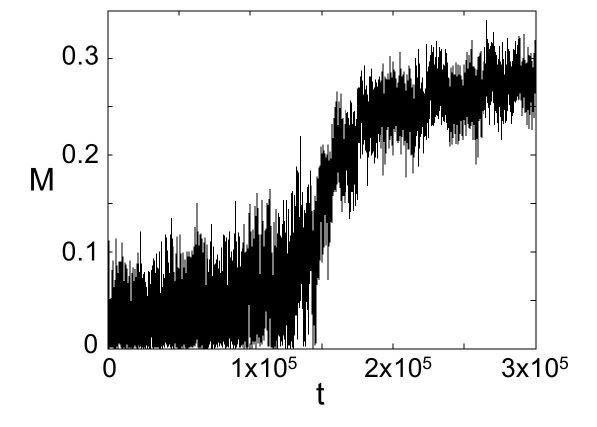
Figure 37: Magnetization vs time for homogeneous initial conditions with semi-elliptical velocity distribution, at $E=0.69$, for a system with $N=2^{12}$ particles.

We have computed the distributions at the times $t=1.5\times 10^{5}$, $t=1.7\times 10^{5}$, $t=2.0\times 10^{5}$, $t=2.4\times 10^{5}$, $t=2.8\times 10^{5}$. From Figure 37 it can be seen that these times are all after the destabilization of the homogeneous phase (the corresponding values of the magnetization, averaged over a short interval of time, are $M=0.17$, $M=0.19$, $M=0.26$, $M=0.26$, and $M=0.28$). In Figure 38 we show the distribution $f(\epsilon)$ obtained at $t=2.8\times 10^{5}$.

Figure 38: One particle distribution function at time $t=2.8\times 10^{5}$. It has been fitted with a polytrope with index $n=4.3$.

In all cases, the points are arranged along a line and therefore at all times the system is in a stationary state of the Vlasov equation. Therefore, for all the time range during the approach to BG equilibrium, the system passes by a sequence of quasi stationary steady solutions of the Vlasov equation, slowly evolving under the effect of “collisions”. This property is due to the scale separation between the relaxation time (larger than $N$) and the dynamical time (of order unity). Furthermore, the system never goes through Vlasov instability, and all the dynamics is governed by the collisional finite size effects.

The distributions have been fitted with polytropic functions, with index $n=2.5$, $3.0$, $3.5$, $4.0$ and $4.3$, respectively. The fit is very good in all cases (it is shown in Figure 38 for the case $n=4.3$). In addition, the fits suggest an increasing index with time. This is of course natural since the BG equilibrium corresponds to a polytrope with index $n=\infty$. We note that the first index calculated in the magnetized phase is somewhat smaller than $n_{c}$, and the second index is very close but slightly smaller than $n_{c}$. In principle this can be considered perfectly legitimate; in fact, even though the numerical distribution function is all the time very close to a polytrope, small discrepancies can give rise to small uncertainties in the value of the index $n$, considering that in the case of inhomogeneous distribution we have to fit a function $f(\epsilon)$ instead of a function $f(v)$, and there are more sources of numerical errors (like, e.g., the determination of the magnetization $M$ in the definition of the individual energy $\epsilon$). Furthermore, a slight change of the maximum energy of the fit could correspond to a slight change of the polytropic index $n$. We remark that for small values of $n$, like those of the previous Section, this problem of the small uncertainty in the value of $n$ is much less relevant, because of the steeper decrease of those polytropes. It is also possible that a value of $n(t)$ smaller than $n_{c}$ in the inhomogeneous phase is real (i.e. it is not a artifact due to the fit). We may well imagine that the homogeneous phase destabilizes when $n(t)=n_{c}$ and that the inhomogeneous polytropes just after the transition have an index smaller than $n_{c}$. In other words, the evolution of $n(t)$ could be non-monotonic.

6 Waterbag initial condition with $M_{0}=1$

In this Section, we consider a different class of initial conditions, i.e., a waterbag distribution for the velocities, and all the angles at $\theta=0$ so that the initial magnetization is $M_{0}=1$ (this distribution is unsteady). That was the first initial condition considered for the HMF model, the one that revealed the existence of QSSs ar ; latora ; lrt . These conditions have been extensively studied, with the purpose to determine the scaling with $N$ of the QSS lifetime and of its magnetization. It is known that there are large fluctuations from run to run, so it is necessary to perform an average on several runs to estimate the mentioned scaling. In Ref. campa1 , it was shown that the fluctuations can be reduced by using the so-called isotropic waterbag conditions, in which the velocities are not randomly extracted from the waterbag, but are taken equally spaced. This is equivalent to using normal waterbag distributions and performing averages over many runs. We adopt this strategy here, but now with the purpose to study the one particle distribution functions in the QSS.

We have performed runs at the energies $E=0.55$, $E=0.57$, $E=0.61$, $E=0.64$, $E=0.65$, $E=0.66$, $E=0.665$, $E=0.67$ and $E=0.69$. As in Section 4, we simulate a system with $2^{18}$ particles. The last energy is the one mostly studied in the literature, where it is shown that the magnetization of the QSS vanishes in the large $N$ limit. We confirm this result here. On the other hand, we found that at all the smaller energies the magnetization of the QSS does not vanish. In Figures 39 and 40 we show the time evolution of the magnetization for the two energies $E=0.61$ and $E=0.69$, respectively.

Figure 39: Magnetization vs time for waterbag initial conditions with $M(0)=1$, at $E=0.61$.

Figure 40: Magnetization vs time for waterbag initial conditions with $M(0)=1$, at $E=0.69$.

In the early stages of the QSS, the occupation of the one particle phase space presents holes that tend to disappear. This peculiarity is shown in some figures where we plot the location of all the particles in the one particle phase space. The plots correspond to the two energies $E=0.61$ and $E=0.69$, and to two different times for each energy. Figure 41 represents the phase space occupancy at $E=0.61$ at the time $t=100$, which is one fifth of the duration time of the run, as it can be seen from Figure 39. The phase space occupancy at the latest time, $t=500$, is plotted in Figure 42.

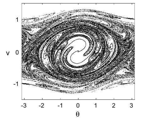
Figure 41: Occupation of the one particle phase space in the early stage ($t=100$) of the QSS at $E=0.61$, for the run with waterbag initial conditions for the velocities, and with $M_{0}=1$. The plot shows a hole in the center.

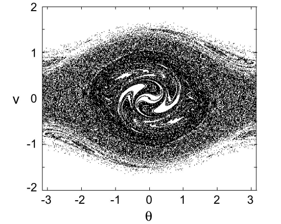
Figure 42: Occupation of the one particle phase space at later times ($t=500$) of the QSS at $E=0.61$. The hole at the center has shrunk considerably.

Although the hole at the center of the phase space has shrunk considerably at $t=500$, it is still very clearly visible. This appears to be in apparent contrast with the numerical distribution function $f(\epsilon)$ at the same time $t=500$, that is shown in Figure 43. As in the previous cases, the disposition along a line of the numerical data confirms that the state is a QSS. However, the interesting point to stress is the presence of a pronounced peak at the smallest energies $\epsilon$. From the expression of the individual energy $\epsilon$, we know that the smallest energies correspond to the particles located near the center of the one particle phase space. Then, we could argue that there is a contradiction between this high peak in $f(\epsilon)$ and the hole in the center of the phase space.

Figure 43: Distribution function $f(\epsilon)$ in the QSS for $E=0.61$. It has been fitted, neglecting the high peak at small energies, by a $n_{0}\simeq 3.56$ polytrope.

To clarify this point we have enlarged the region near the center of the phase space (we do not report here these plots), and this has revealed that the hole contains in fact many particles arranged along thick filaments, that in the two-dimensional plots embracing the whole phase space are not visible. These filaments could be explained by the following argument.

We know that, as long as the evolution of the one particle distribution function $f(\theta,v,t)$ is governed by the Vlasov equation, the mass of each of its phase levels is conserved. However, the evolution causes a complex intertwinement of the various phase levels; this is what allows to consider coarse-grained distributions, and justifies the fact that the numerical distributions, that inevitably have an implicit averaging (at small scales as it may be) have to be compared with the theoretical coarse-grained distributions. For the case under study in this Section, the fine-grained distribution function has only two levels, zero and infinite (i.e., it is a $\delta$ function), since all the particles are initially at $\theta=0$. It may then be argued that for a while there remains very high values also for the coarse-grained distribution function, that are gradually decreased by the mixing. Unless the coarse-grained distribution is analyzed at a very small scale (but this would be possible only with a very large number of particles), high values can be obtained only with particles arranged approximately along a one-dimensional region, i.e., a line.

In Figures 44 and 45 we show the occupancy of the one particle phase space for the energy $E=0.69$, at the times $t=100$ and $t=500$ respectively. Again, at the earlier time the plot presents holes, although they are not at the center. We remind, however, that now the QSS is not magnetized, as shown in Figure 40. At the later time the holes have disappeared.

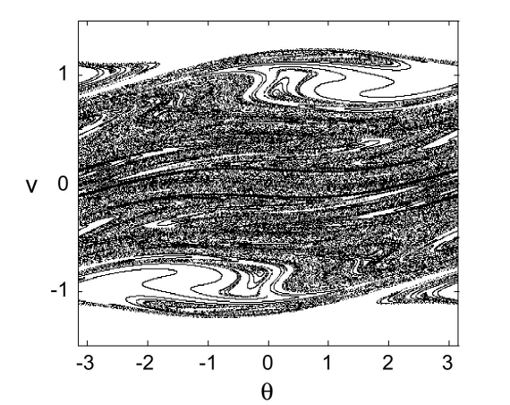
Figure 44: Occupation of the one particle phase space in the early stage ($t=100$) of the QSS at $E=0.69$, for the run with waterbag initial conditions for the velocities, and with $M_{0}=1$. The plot shows two holes.

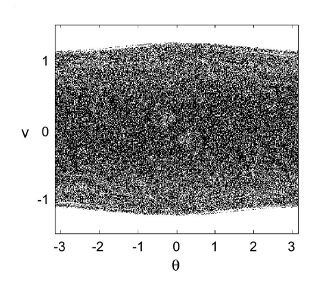
Figure 45: Occupation of the one particle phase space at later times ($t=500$) of the QSS at $E=0.69$. The holes have disappeared.

Also in this case the one particle distribution function at $t=500$ has a pronounced peak at the smaller energy $\epsilon$, as it can be seen in Figure 46. As a matter of fact, the peak is present for all energies $E$ that have been simulated. However, neglecting the high peak at small energy, we see that the distribution function at $E=0.69$ can be fitted with a polytrope with $n=1$. In a previous work campa1 , with numerical simulations performed with much less particles, and therefore with stronger finite size effects and faster QSS evolution, the peak probably had disappeared very soon, and no evidence of it was found (the velocity distribution $f(v)$ could be nicely fitted by a pure $n=1$ polytrope).

Figure 46: Distribution function in the QSS for $E=0.69$. It has been fitted, neglecting the high peak at small energy, by a $n=1$ polytrope.

Figure 47: Numerical caloric curve for the QSS reached from the waterbag $M(0)=1$ initial conditions. It has been fitted by a polytrope with index $n_{0}\simeq 3.56$ for which $C_{kin}\rightarrow\infty$ close to the bifurcation point. The fit is relatively good except for three points that reveal a sort of “hump”. This hump seems to be real (i.e. it is not a numerical artifact). It presents a region of negative kinetic specific heat.

It is interesting to plot the numerical kinetic caloric curve obtained from our simulations. This is done in Figure 47. Except for the curious points around the energy $E=0.66$ (more precisely, the points at $E=0.65$, $E=0.66$ and $E=0.665$) that reveal a sort of “hump”, it seems that $T_{kin}$ is almost constant with $E$. This “plateau” corresponds to a region with infinite kinetic specific heat $C_{kin}=\infty$. Actually, the numerical caloric curve is well-fitted by the physical caloric curve of $n_{0}\simeq 3.56$ polytropes that presents a region of infinite specific heat close to the bifurcation point (see Section 3.6). The distribution function of the QSS at $E=0.61$ is also well-fitted by a $n_{0}$ polytrope, except again for small energies (see Figure 43). These new results do not support the “guess” made in our previous paper cc that the numerical caloric cuve can be fitted by $n=1$ polytropes. They are also in conflict with the early claims of ar ; latora that the numerical caloric curve presents a region of negative kinetic specific heat (this region is not clearly apparent in our simulations, except in the hump). However, we know that a system prepared in the waterbag distribution has a strange dynamics, so that more averages may be needed to obtain reliable results.

7 Conclusion

In spite of the large amount of numerical studies performed on the HMF model, there are two main problems that are still poorly understood. The first one is the anomalous scaling law with $N$ of the homogeneous QSS; the second, treated in this work, is the dependence of the QSS reached by the system from a generic initial condition. The first problem should be restricted to the homogeneous QSSs of one-dimensional systems, where the collisional effects vanish at order ${1}/{N}$. The second problem is expected to be relevant to long-range systems in general.

The Lynden-Bell theory determines, at least in principle, the distribution function of the QSS, although a technical difficulty is to compute it in the generic case of multi-levels initial distributions. On the other hand, various numerical simulations have shown that the theory works only in some cases, failing in others. Since the theory is based on ergodicity or efficient mixing, the reason of the failure has to be traced to an incomplete mixing incomplete . If the system does not mix well, we should not expect any “universality”: The QSS will depend on the degree of mixing. This rises the level of difficulty of the problem since we do not have indications on the further constraints that are imposed by the lack of full mixing.

In this work we have not offered a solution of this problem, in the sense that we have not proposed a way to predict the QSS as a function of the initial condition. Rather, we have proposed to analyze the correspondence between a class of stationary states of the Vlasov equation and the numerical QSS reached by the system starting from various kinds of initial conditions. We have found numerically that, in many cases, the QSS is well-fitted by a polytropic distribution with a compact support. The fact that the distribution has a compact support is consistent with the phenomenology of incomplete relaxation according to which some parts of the phase space (usually those with high energy $\epsilon$) are not sampled by the system. In this respect, the value of the index $n$ may be a measure of mixing.

Polytropic distributions were introduced in different situations:

(i) In astrophysics, they were introduced as particular steady states of the Vlasov equation eddington . Furthermore, it was shown that they extremize a “pseudo-entropy” functional $S=-\int f^{1+1/(n-3/2)}\,d{\bf r}d{\bf v}$ at fixed mass $M$ and energy $E$ ipser , and that maxima of such functionals are dynamically Vlasov stable ih ; aaantonov . This is the interpretation that we have followed in this paper.

(ii) Polytropic distributions were also introduced by Tsallis tsallis from an approach of generalized thermodynamics. In that case, the functional $S$ is interpreted as a generalized entropy and its maximization at fixed mass and energy determines the most probable state of a non-ergodic system for which some regions of phase space are forbidden by the dynamics. Several classes of generalized entropies are possible but the Tsallis entropy is the simplest deviation to the Boltzmann entropy. We leave open the debate about the relevance of this interpretation and refer to cstsallis ; assise for more discussions about this issue.

In this work, we have performed numerical simulations of the HMF model initially prepared in a Vlasov unstable steady state, and we have analyzed the properties of the QSS reached by the system after the rapid relaxation. There have been previous studies dedicated to the description of the QSS in the HMF model, and the following ones have treated the subject under different conditions. In Refs. prl2 ; staniscia1 ; precommun ; bachelard2 , the authors have compared the numerically obtained QSS phase diagram with the theoretical one arising from the application of the Lynden-Bell theory to rectangular waterbag initial conditions. They found that the results agree in some regions of the phase diagram, and disagree in others. Morita and Kaneko mk have analyzed the magnetization of the QSS reached by particular initial conditions, i.e. of the same form as that attained in the BG equilibrium, but with out-of-equilibrium parameter values; the value and the possible oscillations of the QSS magnetization have been studied as a function of the parameters of the initial distribution. Finally, Pakter and Levin levin have studied the same two levels initial distributions as in prl2 , with the purpose to propose an alternative QSS one particle distribution function, with respect to the Lynden-Bell functions, for the cases where the latter does not work.

From the point of view of the initial conditions analyzed, our work is in a sense complementary to those just cited. We have studied several classes of initial distribution functions, some of which with only two levels, as in prl2 ; staniscia1 ; precommun ; bachelard2 and levin , and some with continuous values, as in mk . In addition we have analyzed the properties of the QSS distribution functions, showing that they can be fitted in many cases with polytropic functions. In this respect, the spirit of our work is closer to levin , where the authors try to find the expression for the distribution function. Our results for the QSS reached from waterbag homogeneous initial conditions confirm the results of Ref. levin : we found that the QSS distribution function has a core-halo structure; the limits of the core, in the one particle phase space, are given by a constant energy line, and the core can be fitted by a function $f(\epsilon)$ with a waterbag structure, i.e., a $n={1}/{2}$ polytrope. In addition, we found that the magnetization in the QSS presents oscillations, reminiscent of those found in mk . This could be due to the absence of Landau damping, analogously to what holds for the homogeneous waterbag function, characterized by purely real proper frequencies for the corresponding linearized Vlasov equation.

We found that polytropic functions can fit the QSS distributions also in the other cases, with an index depending on the class of initial condition, although the fit is not very good for all the energies considered. In particular, for energies slightly smaller than the instability threshold the fit appears less satisfying, and probably those cases could be considered with a quasilinear approach quasilinear . The fit with polytropic functions has allowed us to compare the numerical caloric curves with the kinetic caloric curves computed on the basis on the theory of polytropes cc . In particular, using this theory, we have been able to explain the negative kinetic specific heat region observed in the numerical simulations for intermediate energies. This is one of the main results of the paper. For lower energies, the system is not a pure polytrope but it takes a core-halo structure. The core can be fitted by a polytrope, which may differ from the waterbag distribution. The halo may also be fitted by a polytrope so that the core-halo state may be viewed as a “mixture” of two polytropes. Therefore, our results complement, and generalize, the findings in Ref. levin for the waterbag initial condition.

An interesting problem is to understand why the QSS can be fitted by a core-halo state with a polytropic core. Furthermore, the polytropic index of the QSS seems to be correlated to the initial distribution function. Indeed, for the semi-ellipse and waterbag initial conditions, we find that the QSS can be fitted by a polytrope with index $n=1$ and $n=1/2$, respectively. This could be interpreted by saying that the system keeps memory of the initial condition. For the waterbag case, the core does not mix well so it keeps its uniform distribution. On the other hand, a halo is formed probably due to parametric resonance levin . As explained in this paper, the halo is necessary in order to conserve the value of $f_{0}$ in the core while keeping the total energy unchanged. Similar explanations may hold for more general distributions.

We have also studied the approach to BG equilibrium of a system initially prepared in a homogeneous Vlasov stable state. This approach is due to finite size effects. In Ref. campa2 we found that the slowly changing homogeneous distribution function can be fitted by a sequence of polytropes with a time dependent index. Here we extended that work, and we have found that this fit is good also in the successive time range, during which the system progressively magnetizes. We found that the polytropic index increases with time, although the index in the early stages of the magnetized phase appears to be slightly less than the critical index for the homogeneous polytrope. This increase is to be expected since in the BG equilibrium state the index should approach infinity. The reason why polytropic distributions fit well the collisional relaxation of the system remains a mystery. We recall, however, that a similar observation has been made by Taruya & Sakagami ts for self-gravitating systems. Therefore, polytropic distributions seem to be ubiquitous in long-range systems.

Finally, we have considered the QSS reached by a peculiar initial state, in which all the rotators are at $\theta=0$, i.e., with the initial magnetization equal to $1$. In this case, the dynamics is complex due to the formation of phase space holes and thick filaments, and the results have been more difficult to interpret. We found that, except for a few energy values, the numerical caloric curve presents a horizontal segment corresponding to an infinite kinetic specific heat. However, we do not have an explanation for the odd results for the three energies that do not comply with the others and seem to reveal a hump. We also found that the fit with polytropes is here more problematic. For the only energy with a non magnetized QSS, $E=0.69$, we found that the QSS distribution function can be fitted with a semi-ellipse, i.e., an $n=1$ polytrope, only neglecting the pronounced central peak at the smaller energies. We have shown that this peak tends to disappear during the slow QSS evolution. For the others energies with a magnetized QSS, the numerical caloric curve has been compared to the kinetic caloric curve of $n_{0}\simeq 3.56$ polytropes that presents an infinite kinetic specific heat $C_{kin}=+\infty$ (plateau) close to the bifurcation point. The fit is fairly good, except for the three anomalous points mentioned above. The distribution function at $E=0.61$ has also been fitted by a $n_{0}$ polytrope, again excluding the small energies.

Summarizing, we have shown that, for some classes of initial conditions, the QSS can be characterized by polytropic distributions. This appears to be the norm rather than the exception. This does not solve the problem of predicting the QSS structure as a function of the initial conditions since there is no theory to predict the polytropic index $n$, and there exist cases where the QSS is not even a polytrope (hence, polytropic distributions are not “universal attractors”). The problem of predicting the QSS would probably need a proper kinetic equation rather than a theory based on pseudo-entropy functionals (see discussion in incomplete ). However, we hope that these results can give some hint for the search of a more quantitative explanation. We have also shown that for other classes of initial conditions the QSS can be described by a Lynden-Bell distribution (see Fig. 36). The distinction between polytropic (Tsallis) and Lynden-Bell distributions may be related to the ergodic properties of the dynamics. When the system “mixes well”, the Lynden-Bell distribution is reached. Otherwise, the relaxation is incomplete and polytropic distributions may emerge. We conclude that both Lynden-Bell and Tsallis distributions may be relevant to describe QSSs depending on the efficiency of mixing as argued in epjb .

References

- (1) Dynamics and thermodynamics of systems with long range interactions, edited by T. Dauxois, S. Ruffo, E. Arimondo, M. Wilkens, Lecture Notes in Physics 602, (Springer, 2002)
- (2) A. Campa, T. Dauxois, S. Ruffo, Physics Reports 480, 57 (2009)
- (3) J. Messer, H. Spohn, J. Stat. Phys. 29, 561 (1982)
- (4) T. Konishi, K. Kaneko, J. Phys. A 25, 6283 (1992)
- (5) S. Inagaki, T. Konishi, Publ. Astron. Soc. Japan 45, 733 (1993)
- (6) S. Inagaki, Prog. Theor. Phys. 90, 577 (1993)
- (7) C. Pichon, PhD thesis, Cambridge (1994)
- (8) M. Antoni, S. Ruffo, Phys. Rev. E 52, 2361 (1995)
- (9) P.H. Chavanis, J. Vatteville, F. Bouchet, Eur. Phys. J. B 46, 61 (2005)
- (10) P.H. Chavanis, A. Campa, Eur. Phys. J. B 76, 581 (2010)
- (11) V. Latora, A. Rapisarda, C. Tsallis, Phys. Rev. E 64, 056134 (2001)
- (12) V. Latora, A. Rapisarda, C. Tsallis, Physica A 305, 129 (2002)
- (13) C. Tsallis, J. Stat. Phys. 52, 479 (1988)
- (14) P.H. Chavanis, Statistical mechanics of two-dimensional vortices and stellar systems in houches .
- (15) D. Lynden-Bell, MNRAS 136, 101 (1967)
- (16) J. Miller, Phys. Rev. Lett. 65, 2137 (1990)
- (17) R. Robert, J. Sommeria, J. Fluid Mech. 229, 291 (1991)
- (18) P.H. Chavanis, Eur. Phys. J. B 53, 487 (2006)
- (19) A. Antoniazzi, D. Fanelli, S. Ruffo, Y. Yamaguchi, Phys. Rev. Lett. 99, 040601 (2007)
- (20) P.H. Chavanis, G. De Ninno, D. Fanelli, S. Ruffo, in Chaos, Complexity and Transport, edited by C. Chandre, X. Leoncini and G. Zaslavsky (World Scientific, Singapore, 2008) p. 3
- (21) F. Staniscia, P.H. Chavanis, G. De Ninno, D. Fanelli, Phys. Rev. E 80, 021138 (2009)
- (22) F. Staniscia, P.H. Chavanis, G. De Ninno, Phys. Rev. E 83, 051111 (2011)
- (23) A. Antoniazzi, D. Fanelli, J. Barré, P.H. Chavanis, T. Dauxois, S. Ruffo, Phys. Rev. E 75, 011112 (2007)
- (24) A. Antoniazzi, F. Califano, D. Fanelli, S. Ruffo, Phys. Rev. Lett. 98, 150602 (2007)
- (25) R. Bachelard, C. Chandre, D. Fanelli, X. Leoncini, S. Ruffo, Phys. Rev. Lett. 101, 260603 (2008)
- (26) R. Bachelard, C. Chandre, A. Ciani, D. Fanelli, Y.Y. Yamaguchi, Physics Letters A 373, 4239 (2009)
- (27) S. Ogawa, Y. Yamaguchi, Phys. Rev. E 84, 061140 (2011)
- (28) P.H. Chavanis, Physica A 365, 102 (2006)
- (29) P.H. Chavanis, Physica A 387, 787 (2008)
- (30) P.H. Chavanis, Physica A 387, 1504 (2008)
- (31) P.H. Chavanis, C. Sire, Physica A 356, 419 (2005)
- (32) J. Binney, S. Tremaine, Galactic Dynamics (Princeton Series in Astrophysics, 1987)
- (33) A.S. Eddington, MNRAS 76, 572 (1916)
- (34) H.C. Plummer, MNRAS 71, 460 (1911)
- (35) A. Campa, A. Giansanti, G. Morelli, Phys. Rev. E 76, 041117 (2007)
- (36) R. Pakter, Y. Levin, PRL 106, 200603 (2011)
- (37) F. Hohl, J.W. Campbell, Astron. J. 73, 611 (1968)
- (38) S. Goldstein, S. Cuperman, M. Lecar, Mon. Not. R. astr. Soc. 143, 209 (1969)
- (39) S. Cuperman, S. Goldstein, M. Lecar, Mon. Not. R. astr. Soc. 146, 161 (1969)
- (40) M. Lecar, L. Cohen, Astrophys. Space Sci. 13, 397 (1971)
- (41) G. Janin, Astron. Astrophys. 11, 188 (1971)
- (42) J. Tanekusa, Publ. Astron. Soc. Japan 39, 425 (1987)
- (43) P. Mineau, M.R. Feix, J.L. Rouet, Astron. Astrophys. 228, 344 (1990)
- (44) Y.Y. Yamaguchi, Phys. Rev. E 78, 041114 (2008)
- (45) T.N. Teles, Y. Levin, R. Pakter, F.B. Rizzato, J. Stat. Mech., P05007 (2010)
- (46) M. Joyce, T. Worrakitpoonpon, Phys. Rev. E 84, 011139 (2011)
- (47) P.H. Chavanis, J. Stat. Mech. (2011) P08002
- (48) H. Morita, K. Kaneko, PRL 96, 050602 (2006)
- (49) M. Kac, G.E. Uhlenbeck, P.C. Hemmer, J. Math. Phys. 4, 216 (1963)
- (50) W. Braun, K. Hepp, Comm. Math. Phys. 56, 101 (1977)
- (51) A. Campa, P.H. Chavanis, J. Stat. Mech. (2010) P06001
- (52) P.H. Chavanis, AIP Conf. Proc. 970, 39 (2008)
- (53) R. Ellis, K. Haven, B. Turkington, J. Stat. Phys. 101, 999 (2000)
- (54) Y.Y. Yamaguchi, J. Barré, F. Bouchet, T. Dauxois, S. Ruffo, Physica A 337, 36 (2004)
- (55) P.H. Chavanis, L. Delfini, Eur. Phys. J. B 69, 389 (2009)
- (56) F. Staniscia, A. Turchi, D. Fanelli, P.H. Chavanis, G. De Ninno, PRL 105, 010601 (2010)
- (57) A. Campa, P.H. Chavanis, A. Giansanti, G. Morelli, Phys. Rev. E 78, 040102(R) (2008)
- (58) P.H. Chavanis, J. Stat. Mech., P05019 (2010)
- (59) P.H. Chavanis, A. Campa, in preparation
- (60) J. Ipser, ApJ 193, 463 (1974)
- (61) J. Ipser, G. Horwitz, ApJ 232, 863 (1979)
- (62) P.H. Chavanis, A&A 451, 109 (2006)
- (63) B.M. Boghosian, Phys. Rev. E 53, 4754 (1996)
- (64) C. Anteneodo, C. Tsallis, J. Mol. Liq. 71, 255 (1997)
- (65) S. Abe, J. Plasmas Fusion Res. 78, 36 (2002)
- (66) H. Brands, P.H. Chavanis, R. Pasmanter, J. Sommeria, Phys. Fluids 11, 3465 (1999)
- (67) A. Taruya, M. Sakagami, Phys. Rev. Lett. 90, 181101 (2003)
- (68) W. Ettoumi, M.C. Firpo, [arXiv:1206.7002]
- (69) P. Chen, M.C. Cross, Phys. Rev. Lett. 77, 4174 (1996)
- (70) C. Sire, P.H. Chavanis, J. Sopik, Phys. Rev. E 84, 056317 (2011)
- (71) P.H. Chavanis, J. Stat. Mech. 02, 02019 (2012)