Testing for dynamical dark energy models with redshift-space distortions

Abstract

The red-shift space distortions in the galaxy power spectrum can be used to measure the growth rate of matter density perturbations $\delta_{m}$. For dynamical dark energy models in General Relativity we provide a convenient analytic formula of $f(z)\sigma_{8}(z)$ written as a function of the redshift $z$, where $f=d\ln\delta_{m}/d\ln a$ ($a$ is the cosmological scale factor) and $\sigma_{8}$ is the rms amplitude of over-density at the scale $8$ $h^{-1}$ Mpc. Our formula can be applied to the models of imperfect fluids, quintessence, and k-essence, provided that the dark energy equation of state $w$ does not vary significantly and that the sound speed is not much smaller than 1. We also place observational constraints on dark energy models of constant $w$ and tracking quintessence from the recent data of red-shift space distortions.

I Introduction

After the first discovery of cosmic acceleration from the distance measurements of the supernovae type Ia (SN Ia) RP , the existence of dark energy has been also supported from other observational data such as Cosmic Microwave Background (CMB) Spergel ; Komatsu and Baryon Acoustic Oscillations (BAO) BAO . From the theoretical point of view, such a late-time cosmic acceleration is problematic because of the huge difference between the observed dark energy scale and the expected value of the vacuum energy appearing in particle physics Weinberg . Along with the cosmological constant $\Lambda$, many alternative acceleration mechanisms have been proposed, including modifications of the matter/energy content and large-scale modifications of gravity (see Refs. review ; review2 for reviews).

The dark energy equation of state $w$ is constrained by measuring the expansion rate of the Universe from the observations of SN Ia, CMB, and BAO Komatsu ; Suzuki ; BlakeBAO ; BOSS12 ; DNT12 . Although it is possible to rule out some accelerating scenarios from the analysis of the cosmic expansion history alone, we require further precise observational data to clearly distinguish between models with subtly-varying $w$. So far the $\Lambda$-Cold-Dark-Matter ($\Lambda$CDM) model has been consistent with the data, but there are many other dynamical models such as quintessence quinpapers , k-essence kinf ; kespapers , and $f(R)$ gravity fR which are compatible with current observations.

The large-scale structure of the galaxy distribution provides additional important information to discriminate between different dark energy models Tegmark03 . The galaxy clustering occurs due to the gravitational instability of primordial matter density perturbations. The growth rate of matter perturbations can be measured from the redshift-space distortion (RSD) of clustering pattern of galaxies. This distortion is caused by the peculiar velocity of inward collapse motion of the large-scale structure, which is directly related to the growth rate of the matter density contrast $\delta_{m}$ Kaiser . Hence the RSD measurement is very useful to constrain the cosmic growth history.

Recent galaxy redshift surveys have provided bounds on the growth rate $f(z)$ or $f(z)\sigma_{8}(z)$ in terms of the redshift $z=1/a-1$, where $f=d\ln\delta_{m}/d\ln a$ and $\sigma_{8}$ is the rms amplitude of $\delta_{m}$ at the comoving scale $8~{}h^{-1}$ Mpc ($h$ is the normalized Hubble constant $H_{0}=100\,h$ km sec^-1 Mpc^-1) Tegmark04 ; Percival04 ; Porto ; Guzzo08 ; Savas ; Alam ; Blake ; Samushia11 ; Reid12 ; Beutler12 ; Koyama ; Rapetti ; Samushia12 . Although the observational error bars of $f\sigma_{8}$ are not yet small, the data are consistent with the prediction of the $\Lambda$CDM model Blake ; Samushia12 . Recently the RSD data were used to place constraints on modified gravity models such as $f(R)$ gravity and (extended) Galileons Linder12 ; OTT12 . Since the growth rate of matter perturbations in these models is different from that in the $\Lambda$CDM fRper ; Kase ; DTextended , the allowed parameter space is quite tightly constrained even from current observations.

For the models based on General Relativity (GR) without a direct coupling between dark energy and non-relativistic matter, the gravitational coupling appearing in the matter perturbation equation is equivalent to the Newton’s gravitational constant, as long as the dark energy perturbation is negligible relative to the matter perturbation. Nonetheless the evolution of perturbations depends on the background cosmology, so that the dynamical dark energy models with $w$ different from $-1$ can be distinguished from the $\Lambda$CDM. In particular, the future RSD observations may reach the level of discriminating between different dark energy models constructed in the framework of GR.

In this paper we derive an analytic formula of $f(z)\sigma_{8}(z)$ valid for dynamical dark energy models including imperfect fluids, quintessence, and k-essence. Provided that the sound speed $c_{s}$ is not much smaller than $1$ and that the variation of $w$ is not significant, our formula can reproduce the full numerical solutions with high accuracy. The derivation of $f(z)\sigma_{8}(z)$ is based on the expansion of $w$ in terms of the dark energy density parameter $\Omega_{x}$, i.e., $w=w_{0}+\sum_{n=1}w_{n}(\Omega_{x})^{n}$. Since $f(z)\sigma_{8}(z)$ is expressed in terms of the present values of $\sigma_{8}$ and $\Omega_{x}$ as well as $w_{n}$ ($n=0,1,2,\cdots$), our formula is convenient to test for dynamical dark energy models with the observational data of the cosmic growth rate. For the models with constant $w$ there are 3 parameters $w_{0}$, $\sigma_{8}(z=0)$, and $\Omega_{x}(z=0)$ in the analytic expression of $f(z)\sigma_{8}(z)$. In tracking quintessence models Zlatev , where the dark energy equation of state is nearly constant during the matter era ($w=w_{(0)}$), we show that our formula of $f(z)\sigma_{8}(z)$ also contains only 3 parameters: $w_{(0)}$, $\sigma_{8}(z=0)$, and $\Omega_{x}(z=0)$. Using the recent RSD data, we carry out the likelihood analysis by varying these 3 parameters to find observational bounds on $w_{0}$ and $w_{(0)}$.

This paper is organized as follows. In Sec. II we review cosmological perturbation theory in general dark energy models including imperfect fluids, quintessence, and k-essence. In Sec. III dynamical dark energy models are classified depending on how the equation of state $w$ is expanded in terms of $\Omega_{x}$. In Sec. IV we derive an analytic formula for $f(z)\sigma_{8}(z)$ and in Sec. V we confirm the validity of this formula in concrete examples of dark energy models. In Sec. VI we perform the likelihood analysis to test for constant $w$ and tracking quintessence models with the recent RSD data. Sec. VII is devoted to our main conclusions.

II Cosmological perturbations and redshift-space distortions

As the dark energy component we consider a fluid characterized by the equation of state $w=P_{x}/\rho_{x}$, where $P_{x}$ is the pressure and $\rho_{x}$ is the energy density. We also take into account non-relativistic matter (cold dark matter and baryons) with the energy density $\rho_{m}$ and treat it as a perfect fluid with the equation of state $w_{m}=0$. We deal with such a two-fluid system in the framework of GR under the assumption that dark energy is uncoupled to non-relativistic matter. Our analysis covers quintessence quinpapers and k-essence kinf ; kespapers models, in which the Lagrangian $P$ of dark energy depends on a scalar field $\phi$ and a kinetic term $X=-(\nabla\phi)^{2}/2$. In these models we have that $P_{x}=P$ and $\rho_{x}=2XP_{,X}-P$, where $P_{,X}\equiv\partial P/\partial X$.

In the flat Friedmann-Lemaître-Robertson-Walker (FLRW) background with the scale factor $a(t)$, where $t$ is the cosmic time, dark energy and non-relativistic matter obey, respectively, the following continuity equations

$$\rho_{x}^{\prime}+3(1+w)\rho_{x}=0\,,$$ (1)

$$\rho_{m}^{\prime}+3\rho_{m}=0\,,$$ (2)

where a prime represents a derivative with respect to $N=\ln a$. We introduce the density parameters $\Omega_{x}=8\pi G\rho_{x}/(3H^{2})$ and $\Omega_{m}=8\pi G\rho_{m}/(3H^{2})$, where $G$ is the gravitational constant and $H=\dot{a}/a$ is the Hubble parameter (a dot represents derivative with respect to $t$). From the Einstein equations it follows that

$$\Omega_{x}+\Omega_{m}=1\,,$$ (3)

$$\frac{H^{\prime}}{H}=-\frac{3}{2}(1+w\Omega_{x})\,.$$ (4)

The dark energy density parameter satisfies the differential equation

$$\Omega_{x}^{\prime}=-3w\Omega_{x}(1-\Omega_{x})\,.$$ (5)

Let us consider scalar metric perturbations about the flat FLRW background. We neglect the contribution of tensor and vector perturbations. In the absence of the anisotropic stress the perturbed line element in the longitudinal gauge is given by Bardeen

$$ds^{2}=-(1-2\Phi)\,dt^{2}+a^{2}(t)(1+2\Phi)d{\bm{x}}^{2}\,,$$ (6)

where $\Phi$ is the gravitational potential. We decompose the energy densities $\rho_{i}$ (where $i=x,m$) and the pressure $P_{x}$ into the background and inhomogeneous parts, as $\rho_{i}=\rho_{i}(t)+\delta\rho_{i}(t,{\bm{x}})$ and $P_{x}=P_{x}(t)+\delta P_{x}(t,{\bm{x}})$. We also define the following quantities

$$\delta_{i}\equiv\frac{\delta\rho_{i}}{\rho_{i}}\,,\qquad\theta_{i}\equiv\frac{\nabla^{2}v_{i}}{aH}\qquad(i=x,m),$$ (7)

where $v_{x}$ and $v_{m}$ are the rotational-free velocity potentials of dark energy and non-relativistic matter, respectively.

In Fourier space dark energy perturbations obey the following equations of motion Kodama ; Bean ; Sapone ; DEbook

$$\delta_{x}^{\prime}+3(c_{x}^{2}-w)\delta_{x}=-(1+w)\left(3\Phi^{\prime}+\theta_{x}\right)\,,$$ (8)

$$\theta_{x}^{\prime}+\left(2-3w+\frac{H^{\prime}}{H}+\frac{w^{\prime}}{1+w}\right)\theta_{x}=\left(\frac{k}{aH}\right)^{2}\left(\frac{c_{x}^{2}}{1+w}\delta_{x}-\Phi\right)\,,$$ (9)

where $c_{x}^{2}=\delta P_{x}/\delta\rho_{x}$ and $k$ is a comoving wave number. The perturbed equations of non-relativistic matter (perfect fluids) are

$$\delta_{m}^{\prime}=-3\Phi^{\prime}-\theta_{m}\,,$$ (10)

$$\theta_{m}^{\prime}+\left(2+\frac{H^{\prime}}{H}\right)\theta_{m}=-\left(\frac{k}{aH}\right)^{2}\Phi\,.$$ (11)

From the Einstein equations we obtain

$$\left(\frac{k}{aH}\right)^{2}\Phi=\frac{3}{2}\left(\Omega_{m}\hat{\delta}_{m}+\Omega_{x}\hat{\delta}_{x}\right)\,,$$ (12)

$$\Phi^{\prime}+\Phi=-\frac{3}{2}\left(\frac{aH}{k}\right)^{2}\left[\Omega_{m}\theta_{m}+(1+w)\Omega_{x}\theta_{x}\right]\,,$$ (13)

where $\hat{\delta}_{m}$ and $\hat{\delta}_{x}$ are the rest frame gauge-invariant density perturbations defined by

$$\hat{\delta}_{m}=\delta_{m}+3\left(\frac{aH}{k}\right)^{2}\theta_{m}\,,\qquad\hat{\delta}_{x}=\delta_{x}+3\left(\frac{aH}{k}\right)^{2}(1+w)\theta_{x}\,.$$ (14)

For imperfect fluids such as quintessence and k-essence there exist non-adiabatic entropy perturbations generated from dissipative processes. We introduce a gauge-invariant entropy perturbation $\delta s_{x}$ of dark energy, as Kodama ; Bean ; BTW05

$$\delta s_{x}=(c_{x}^{2}-c_{a}^{2})\delta_{x}=\frac{\dot{P}_{x}}{\rho_{x}}\left(\frac{\delta P_{x}}{\dot{P}_{x}}-\frac{\delta\rho_{x}}{\dot{\rho}_{x}}\right)\,,$$ (15)

where $c_{a}$ is the adiabatic sound speed defined by

$$c_{a}^{2}=\frac{\dot{P}_{x}}{\dot{\rho}_{x}}=w-\frac{w^{\prime}}{3(1+w)}\,.$$ (16)

In the rest frame where the entropy perturbation is given by $\delta s_{x}=(\hat{c}_{x}^{2}-c_{a}^{2})\hat{\delta}_{x}$, the sound speed squared $c_{s}^{2}\equiv\hat{c}_{x}^{2}$ is gauge-invariant. Using the definition of $\hat{\delta}_{x}$ in Eq. (14), the pressure perturbation of dark energy can be expressed as

$$\delta P_{x}=c_{s}^{2}\,\delta\rho_{x}+3\left(\frac{aH}{k}\right)^{2}(1+w)(c_{s}^{2}-c_{a}^{2})\rho_{x}\theta_{x}\,,$$ (17)

whereas the sound speed squared $c_{x}^{2}=\delta P_{x}/\delta\rho_{x}$ in the random frame is related to $c_{s}^{2}$ via

$$c_{x}^{2}=c_{s}^{2}+3\left(\frac{aH}{k}\right)^{2}(1+w)(c_{s}^{2}-c_{a}^{2})\frac{\theta_{x}}{\delta_{x}}\,.$$ (18)

In terms of $c_{s}^{2}$, Eqs. (8) and (9) can be written as

$$\delta_{x}^{\prime}+3(c_{s}^{2}-w)\delta_{x}=-3(1+w)\Phi^{\prime}-(1+w)\left[1+9\left(\frac{aH}{k}\right)^{2}(c_{s}^{2}-c_{a}^{2})\right]\theta_{x}\,,$$ (19)

$$\theta_{x}^{\prime}+\left(2+\frac{H^{\prime}}{H}-3c_{s}^{2}\right)\theta_{x}=\left(\frac{k}{aH}\right)^{2}\left(\frac{c_{s}^{2}}{1+w}\delta_{x}-\Phi\right)\,.$$ (20)

In k-essence characterized by the Lagrangian density $P(\phi,X)$, the perturbed quantities can be expressed as

$$\delta\rho_{x} = \left(P_{,X}+2XP_{,XX}\right)\delta X-\left(P_{,\phi}-2XP_{,X\phi}\right)\delta\phi\,,$$ (21)

$$\delta P_{x} = P_{,X}\delta X+P_{,\phi}\delta\phi\,,$$ (22)

$$\theta_{x} = \frac{k^{2}}{a\dot{\phi}}\delta\phi\,,$$ (23)

where $\delta\phi$ is the field perturbation and $\delta X=\dot{\phi}\,\dot{\delta\phi}+\dot{\phi}^{2}\Phi$. From Eq. (17) the rest frame sound speed can be obtained by setting $\delta\phi=0$ in Eqs. (21) and (22), i.e., $c_{s}^{2}=P_{,X}/(P_{,X}+2XP_{,XX})$ Garriga . In quintessence characterized by the Lagrangian $P=X-V(\phi)$, the sound speed squared reduces to $c_{s}^{2}=1$.

From Eqs. (10) and (11) it follows that

$$\delta_{m}^{\prime\prime}+\left(2+\frac{H^{\prime}}{H}\right)\delta_{m}^{\prime}-\left(\frac{k}{aH}\right)^{2}\Phi=-3\left[\Phi^{\prime\prime}+\left(2+\frac{H^{\prime}}{H}\right)\Phi^{\prime}\right]\,.$$ (24)

For the perturbations deep inside the Hubble radius ($k\gg aH$) relevant to large-scale structures, the r.h.s. of Eq. (24) can be neglected relative to the l.h.s. of it, in addition to the fact that $\hat{\delta}_{m}\simeq\delta_{m}$. If the contribution of dark energy perturbations can be neglected relative to that of matter perturbations in Eq. (12), i.e. $|\Omega_{m}\hat{\delta}_{m}|\gg|\Omega_{x}\hat{\delta}_{x}|$, Eq. (24) reads

$$\delta_{m}^{\prime\prime}+\frac{1}{2}\left(1-3w\Omega_{x}\right)\delta_{m}^{\prime}-\frac{3}{2}\Omega_{m}\delta_{m}\simeq 0\,,$$ (25)

where we made use of Eq. (4).

During the deep matter era in which $\Omega_{m}\simeq 1$, there is a growing-mode solution $\delta_{m}=\delta_{m}^{\prime}\propto a$ to Eq. (25). In this regime Eq. (12) tells us that $\Phi=\,{\rm constant}$ and hence $\theta_{m}\simeq-\delta_{m}^{\prime}$ from Eq. (10). For the dark energy density contrast $\delta_{x}$, it is natural to choose the adiabatic initial condition Kodama ; DEbook

$$\delta_{x}=(1+w)\delta_{m}\,.$$ (26)

The initial condition of $\theta_{x}$ is known by substituting Eq. (26) and $\delta_{x}^{\prime}=(1+w+w^{\prime})\delta_{m}$ into Eq. (19). We will discuss the accuracy of the approximate equation (25) in Sec. III.

$z$	$f\sigma_{8}$	survey
0.067	0.423$\pm$ 0.055	6dFGRS (2012) Beutler12
0.17	0.51$\pm$ 0.06	2dFGRS (2004) Percival04
0.22	0.42$\pm$ 0.07	WiggleZ (2011) Blake
0.25	0.3512$\pm$ 0.0583	SDSS LRG (2011) Samushia11
0.37	0.4602$\pm$ 0.0378	SDSS LRG (2011) Samushia11
0.41	0.45$\pm$ 0.04	WiggleZ (2011) Blake
0.57	0.415$\pm$ 0.034	BOSS CMASS (2012) Reid12
0.6	0.43$\pm$ 0.04	WiggleZ (2011) Blake
0.78	0.38$\pm$ 0.04	WiggleZ (2011)Blake

Table 1: Data of $f\sigma_{8}$ versus the redshift $z$ measured from the RSD.

The growth rate of matter perturbations can be measured from the RSD in clustering pattern of galaxies because of radial peculiar velocities. The perturbation $\delta_{g}$ of galaxies is related to the matter perturbation $\delta_{m}$, as $\delta_{g}=b\delta_{m}$, where $b$ is a bias factor. The galaxy power spectrum ${\cal P}_{g}({\bm{k}})$ in the redshift space can be expressed as Kaiser ; Tegmark06 ; Song09 ; White

$${\cal P}_{g}({\bm{k}})={\cal P}_{gg}({\bm{k}})-2\mu^{2}{\cal P}_{g\theta}({\bm{k}})+\mu^{4}{\cal P}_{\theta\theta}({\bm{k}})\,,$$ (27)

where $\mu={\bm{k}}\cdot{\bm{r}}/(kr)$ is the cosine of the angle of the ${\bm{k}}$ vector to the line of sight (vector ${\bm{r}}$), ${\cal P}_{gg}({\bm{k}})$ and ${\cal P}_{\theta\theta}({\bm{k}})$ are the real space power spectra of galaxies and $\theta$, respectively, and ${\cal P}_{g\theta}({\bm{k}})$ is the cross power spectrum of galaxy-$\theta$ fluctuations in real space.

In Eq. (10) the variation of the gravitational potential is neglected relative to the growth rate of $\delta_{m}$, so that

$$\theta_{m}\simeq-f\delta_{m}\,,\qquad f\equiv\frac{\dot{\delta}_{m}}{H\delta_{m}}\,.$$ (28)

Under the continuity equation (28), ${\cal P}_{gg}$, ${\cal P}_{g\theta}$, and ${\cal P}_{\theta\theta}$ in Eq. (27) depend on $(b\delta_{m})^{2}$, $(b\delta_{m})(f\delta_{m})$, and $(f\delta_{m})^{2}$, respectively. We normalize the amplitude of $\delta_{m}$ at the scale $8\,h^{-1}$ Mpc, for which we write $\sigma_{8}$. Assuming that the growth of perturbations is scale-independent, the constraints on $b\delta_{m}$ and $f\delta_{m}$ translate into those on $b\sigma_{8}$ and $f\sigma_{8}$. The advantage of using $f\sigma_{8}$ is that the growth rate is directly known without the bias factor $b$. In Table 1 we show the current data of $f\sigma_{8}$ as a function of $z$ from the RSD measurements.

III Dynamical dark energy models

In this section, we discuss a number of dynamical dark energy models in which the field equations presented in the previous section can be applied.

III.1 Imperfect fluids

For imperfect fluids the rest frame sound speed $c_{s}$ is generally different from the adiabatic sound speed $c_{a}$. For constant $w$ one has $c_{a}^{2}=w$. If $c_{s}^{2}$ is constant as well, the evolution of dark energy perturbations is known by solving Eqs. (19) and (20) together with the background equations (3)-(5). This is the approach taken in Ref. Bean . Note also that for $c_{s}$ of the order of 1 the contribution of dark energy perturbations to $\Phi$ in Eq. (12) is negligibly small relative to matter perturbations Bean ; Riotto .

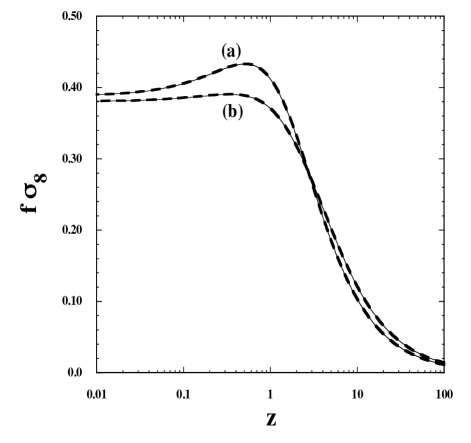
Figure 1: Evolution of $f\sigma_{8}$ versus the redshift $z$ for $c_{s}^{2}=1$, $k=0.07\,h$ Mpc^-1, $\sigma_{8}(z=0)=0.811$, and $\Omega_{m}(z=0)=0.73$. The cases (a) and (b) correspond to $w=-0.8$ and $w=-0.5$, respectively. The solid lines show the numerically integrated solutions, whereas the bald dashed lines correspond to the solutions derived by using the approximate equation (25).

In Fig. 1 we plot the evolution of $f\sigma_{8}$ for $c_{s}^{2}=1$ and $k=0.07\,h$ Mpc^-1 with two different values of $w$. The approximate equation (25) reproduces the full numerical solution within the 0.1 % accuracy. This means that, for $c_{s}^{2}=1$, the contribution of dark energy perturbations to the gravitational potential is suppressed relative to that of matter perturbations. For $c_{s}^{2}=0$ and $w=-0.8$ we find that the difference of $f\sigma_{8}(z=0)$ between the numerical result and the approximated solution is about 4 % for the mode $k=0.07\,h$ Mpc^-1. For $w$ larger than $-0.8$ the difference gets even larger, but such values of $w$ are not allowed observationally Komatsu ; Suzuki . In Ref. Sapone it was found that galaxy redshift and tomographic redshift surveys can constrain the sound speed only if $c_{s}^{2}$ is sufficiently small, of the order of $c_{s}^{2}\lesssim 10^{-4}$.

III.2 Quintessence

Quintessence quinpapers is characterized by the Lagrangian $P(\phi,X)=X-V(\phi)$, where $V(\phi)$ is the field potential. In this case the sound speed $c_{s}$ is equivalent to 1, so that the contribution of dark energy perturbations to the gravitational potential is negligible. There are several classes of potentials which give rise to different evolution of $w$.

The first class is the model with constant $w$, which can be realized by the following potential review ; Saini03 ; Sahni06

$$V(\phi)=\frac{3H_{0}^{2}(1-w)(1-\Omega_{m0})^{1/|w|}}{16\pi G\Omega_{m0}^{\alpha}}\sinh^{-2\alpha}\left(|w|\sqrt{\frac{6\pi G}{1+w}}(\phi-\phi_{0}+\phi_{1})\right),$$ (29)

where $\alpha=(1+w)/|w|$, $\phi_{0}$ and $\Omega_{m0}$ are the today’s values of $\phi$ and $\Omega_{m}$ respectively, and

$$\phi_{1}=\sqrt{\frac{1+w}{6\pi G}}\frac{1}{|w|}\ln\frac{1+\sqrt{1-\Omega_{m0}}}{\sqrt{\Omega_{m0}}}\,.$$ (30)

This case is identified as an imperfect fluid with $c_{s}^{2}=1$ and $w=\,$constant discussed in Sec. III.1.

The second class consists of freezing models CL05 , in which the evolution of the field gradually slows down at late times. A typical example is the inverse power-law potential Ratra

$$V(\phi)=M^{4+p}\phi^{-p}\,,$$ (31)

where $p$ is a positive constant. For this potential there exists a so-called tracker solution Zlatev with a nearly constant field equation of state $w=w_{(0)}\equiv-2/(p+2)$ during the matter era, which is followed by the decrease of $w$. Considering a homogeneous perturbation $\delta w$ around $w_{(0)}$, the field equation of state is expressed as Chiba

$$w=w_{(0)}+\sum_{n=1}^{\infty}\frac{(-1)^{n-1}w_{(0)}(1-w_{(0)}^{2})}{1-(n+1)w_{(0)}+2n(n+1)w_{(0)}^{2}}\left(\frac{\Omega_{x}}{1-\Omega_{x}}\right)^{n}\,.$$ (32)

Expansion of $w$ around $\Omega_{x}$ reads

$$w = w_{(0)}+\frac{(1-w_{(0)}^{2})w_{(0)}}{1-2w_{(0)}+4w_{(0)}^{2}}\Omega_{x}+\frac{(1-w_{(0)}^{2})w_{(0)}^{2}(8w_{(0)}-1)}{(1-2w_{(0)}+4w_{(0)}^{2})(1-3w_{(0)}+12w_{(0)}^{2})}\Omega_{x}^{2}$$ (33)

$$+\frac{2(1-w_{(0)}^{2})w_{(0)}^{3}(4w_{(0)}-1)(18w_{(0)}+1)}{(1-2w_{(0)}+4w_{(0)}^{2})(1-3w_{(0)}+12w_{(0)}^{2})(1-4w_{(0)}+24w_{(0)}^{2})}\Omega_{x}^{3}+{\cal O}(\Omega_{x}^{4})\,,$$

which varies with the growth of $\Omega_{x}$.

The third class consists of thawing models CL05 , in which the field is nearly frozen by a Hubble friction during the early cosmological epoch and it starts to evolve once the field mass $m$ drops below $H$. In this case $w$ is initially close to $-1$ and then $w$ starts to grow at late times. The representative potential of this class is that of the pseudo Nambu-Goldstone boson PNGB , i.e.,

$$V(\phi)=\Lambda^{4}\left[1+\cos(\phi/f)\right]\,,$$ (34)

where $\Lambda$ and $f$ are constants. Assuming that the evolution of the scale factor can be approximated as that of the $\Lambda$CDM model, the field equation of state is estimated as Dutta (see also Ref. Scherrer )

$$w=-1+(1+\tilde{w}_{0})a^{3(K-1)}\left[\frac{(K-F(a))(F(a)+1)^{K}+(K+F(a))(F(a)-1)^{K}}{(K-\Omega_{x0}^{-1/2})(\Omega_{x0}^{-1/2}+1)^{K}+(K+\Omega_{x0}^{-1/2})(\Omega_{x0}^{-1/2}-1)^{K}}\right]^{2}\,,$$ (35)

where $\tilde{w}_{0}$ and $\Omega_{x0}$ are the today’s values of $w$ and $\Omega_{x}$ respectively, and

$$K=\sqrt{1-\frac{V_{,\phi\phi}(\phi_{i})}{6\pi GV(\phi_{i})}}\,,\qquad F(a)=\sqrt{1+(\Omega_{x0}^{-1}-1)a^{-3}}\,.$$ (36)

The constant $K$ is related to the mass of the field at the initial displacement, $\phi=\phi_{i}$. Expansion around $\Omega_{x}=0$ gives

$$w=-1+w_{1}\Omega_{x}+\frac{1}{5}(K^{2}+1)w_{1}\Omega_{x}^{2}+\frac{1}{175}(3K^{4}+31K^{2}+3)w_{1}\Omega_{x}^{3}+{\cal O}(\Omega_{x}^{4})\,,$$ (37)

where

$$w_{1}=\frac{4}{9}\,\frac{1+\tilde{w}_{0}}{[(K-\Omega_{x0}^{-1/2})(\Omega_{x0}^{-1/2}+1)^{K}+(K+\Omega_{x0}^{-1/2})(\Omega_{x0}^{-1/2}-1)^{K}]^{2}}\left(\frac{1-\Omega_{x0}}{\Omega_{x0}}\right)^{K-1}K^{2}(K-1)^{2}(K+1)^{2}\,.$$ (38)

The growth of $\Omega_{x}$ leads to the deviation from $w=-1$.

III.3 K-essence

The equation of state for K-essence with the Lagrangian density $P(\phi,X)$ is given by $w=P/(2XP_{,X}-P)$. This shows that cosmic acceleration with $w\approx-1$ can be realized either for (a) $X\approx 0$ or (b) $P_{,X}\approx 0$.

In the case (a) Chiba et al. Chibake showed that, for the factorized function $P(\phi,X)=V(\phi)F(X)$, the field equation of state is given by the same form as Eq. (35) with the replacement $K=\sqrt{1-V_{,\phi\phi}(\phi_{i})/(6\pi GF_{,X}(0)V^{2}(\phi_{i}))}$, where $F(X)$ is expanded around $X=0$ as $F(X)=F(0)+F_{,X}(0)X$. In this case the sound speed squared is also close to 1, so that the situation is similar to that in thawing quintessence models.

In the case (b) the evolution of $w$ depends on the functional form of $P(\phi,X)$, so it is difficult to derive a general expression of $w$ Chibake . One of the examples which belongs to this class is the dilatonic ghost condensate model Piazza characterized by the Lagrangian $P(\phi,X)=-X+e^{\kappa\lambda\phi}X^{2}/M^{4}$, where $\kappa=\sqrt{8\pi G}$, $\lambda$ and $M$ are constants (see also Ref. Mukohyama ). In this model the fixed points during the radiation and matter eras correspond to $P_{,X}=0$ and $w=-1$, i.e., $y\equiv Xe^{\kappa\lambda\phi}/M^{4}=1/2$. On the other hand the (no-ghost) accelerated fixed point corresponds to $y=1/2+\lambda^{2}f(\lambda)/16$ with the equation of state $w=-[1-\lambda^{2}f(\lambda)/8]/[1+3\lambda^{2}f(\lambda)/8]>-1$, where $f(\lambda)=1+\sqrt{1+16/(3\lambda^{2})}$. Hence the evolution of $w$ is similar to that in thawing quintessence models.

The sound speed squared in the dilatonic ghost condensate model is given by $c_{s}^{2}=(2y-1)/(6y-1)$, so that $c_{s}^{2}\simeq 0$ during radiation and matter eras. The late-time cosmic acceleration occurs for $1/2\leq y<2/3$ and hence $0\leq c_{s}^{2}<1/9$ at this fixed point. The fact that $c_{s}^{2}$ is close to 0 during most of the cosmological epoch is a different signature relative to quintessence. However, since $w$ is very close to $-1$ during radiation and matter eras, the adiabatic initial condition (26) shows that the dark energy perturbation $\delta_{x}$ is initially suppressed relative to the matter perturbation $\delta_{m}$. As long as the today’s value of $w$ is not significantly away from $-1$ the contribution of the dark energy perturbation to $\Phi$ is suppressed relative to the matter perturbation, so that the approximate equation (25) can be trustable even in such cases.

IV Analytic solutions of $f\sigma_{8}$

We derive analytic solutions of $f\sigma_{8}$ by solving the approximate equation (25). Recall that the equation of state for tracking and thawing models of quintessence can be expressed in terms of the field density parameter $\Omega_{x}$, see Eqs. (33) and (37). We generally expand the dark energy equation of state in terms of the density parameter $\Omega_{x}$, as

$$w=w_{0}+\sum_{n=1}^{\infty}w_{n}(\Omega_{x})^{n}\,.$$ (39)

Since $\Omega_{x}$ grows as large as 0.7 today, we expect that it may be necessary to pick up the terms higher than the first few terms in Eq. (39).

In terms of the function $f=\delta_{m}^{\prime}/\delta_{m}$, Eq. (25) can be written as Wang

$$3w\Omega_{x}(1-\Omega_{x})\frac{df}{d\Omega_{x}}=f^{2}+\frac{1}{2}(1-3w\Omega_{x})f-\frac{3}{2}(1-\Omega_{x})\,,$$ (40)

where we employed Eq. (5). Introducing the growth index $\gamma$ as $f=(\Omega_{m})^{\gamma}=(1-\Omega_{x})^{\gamma}$ Peebles , Eq. (40) reads

$$3w\Omega_{x}(1-\Omega_{x})\ln(1-\Omega_{x})\frac{d\gamma}{d\Omega_{x}}=\frac{1}{2}-\frac{3}{2}w(1-2\gamma)\Omega_{x}+(1-\Omega_{x})^{\gamma}-\frac{3}{2}(1-\Omega_{x})^{1-\gamma}\,.$$ (41)

We derive the solution of Eq. (41) by expanding $\gamma$ in terms of $\Omega_{x}$, i.e., $\gamma=\gamma_{0}+\sum_{n=1}\gamma_{n}(\Omega_{x})^{n}$. While $\Omega_{m}$ is smaller than $\Omega_{x}$ today, the former is not suitable as an expansion parameter as we would like to derive an analytic formula valid at high redshifts as well. In fact, it is expected that future RSD surveys such as Subaru/FMOS will provide high-redshift data up to $z=2$. Using the expansion of $w$ in Eq. (39) as well, we obtain the following approximate solution

$$\gamma = \frac{3(1-w_{0})}{5-6w_{0}}+\frac{3}{2}\frac{(1-w_{0})(2-3w_{0})+2w_{1}(5-6w_{0})}{(5-6w_{0})^{2}(5-12w_{0})}\Omega_{x}$$ (42)

$$+[(w_{0}-1)(3w_{0}-2)(324w_{0}^{2}-420w_{0}+97)+12(5-6w_{0})^{2}(5w_{2}-12w_{2}w_{0}+12w_{1}^{2})$$

$$~{}~{}~{}+6(5-6w_{0})(72w_{0}^{2}-90w_{0}+23)w_{1}]/[4(5-6w_{0})^{3}(5-12w_{0})(5-18w_{0})]\,\Omega_{x}^{2}+{\cal O}(\Omega_{x}^{3})\,.$$

The 1-st order solution is identical to the one found in Ref. Gong by setting $w_{1}=0$. For $w_{0}=-1$, $w_{1}=0$, and $w_{2}=0$ it follows that $\gamma\simeq 0.545+7.29\times 10^{-3}\Omega_{x}+4.04\times 10^{-3}\Omega_{x}^{2}$. In this case the second and third terms are indeed much smaller than the first one, so that $\gamma$ is nearly constant. For the models with $w_{0}=-1$, $w_{1}=0.3$, and $w_{2}=0$ (in which case the value of $w$ today is around $-0.8$) one has $\gamma\simeq 0.545+1.21\times 10^{-2}\Omega_{x}+6.55\times 10^{-3}\Omega_{x}^{2}$. Even in this case the variation of $\gamma$ induced by the second and third terms is small (see also Refs. Linder for related works).

From the definition of $f$ the matter perturbation obeys the differential equation $(\ln\delta_{m})^{\prime}=(1-\Omega_{x})^{\gamma}$. Using Eq. (5), we obtain

$$\frac{d}{d\Omega_{x}}\ln\delta_{m}=-\frac{(1-\Omega_{x})^{\gamma-1}}{3w\Omega_{x}}\,.$$ (43)

In the following we derive the solution of this equation under the approximation that $\gamma$ is constant. We expand the term $(1-\Omega_{x})^{\gamma-1}$ around $\Omega_{x}=0$, as

$$(1-\Omega_{x})^{\gamma-1}=1+\sum_{n=1}^{\infty}\alpha_{n}(\Omega_{x})^{n}\,,\qquad\alpha_{n}=\frac{(-1)^{n}}{n!}(\gamma-1)(\gamma-2)\cdots(\gamma-n)\,.$$ (44)

In order to evaluate the r.h.s. of Eq. (43), we expand $1/w$ in the form

$$\frac{1}{w}=\frac{1}{w_{0}}\left[1+\sum_{n=1}^{\infty}\beta_{n}(\Omega_{x})^{n}\right]\,,$$ (45)

where the coefficients $\beta_{n}$’s can be expressed by $w_{n}$’s, say $\beta_{1}=-w_{1}/w_{0}$. Then Eq. (43) can be written as

$$\frac{d}{d\Omega_{x}}\ln\delta_{m}=-\frac{1}{3w_{0}\Omega_{x}}\left[1+\sum_{n=1}^{\infty}c_{n}(\Omega_{x})^{n}\right]\,,$$ (46)

where

$$c_{n}=\sum_{i=0}^{n}\alpha_{n-i}\beta_{i}\,,$$ (47)

with $\alpha_{0}=\beta_{0}=1$. The first three coefficients $c_{i}$ are

$$c_{1} = -(\gamma-1)-\frac{w_{1}}{w_{0}}\,,$$ (48)

$$c_{2} = \frac{1}{2}(\gamma-1)(\gamma-2)+(\gamma-1)\frac{w_{1}}{w_{0}}-\frac{w_{2}w_{0}-w_{1}^{2}}{w_{0}^{2}}\,,$$ (49)

$$c_{3} = -\frac{1}{6}(\gamma-1)(\gamma-2)(\gamma-3)-\frac{1}{2}(\gamma-1)(\gamma-2)\frac{w_{1}}{w_{0}}+(\gamma-1)\frac{w_{2}w_{0}-w_{1}^{2}}{w_{0}^{2}}-\frac{w_{3}w_{0}^{2}-2w_{1}w_{2}w_{0}+w_{1}^{3}}{w_{0}^{3}}\,.$$ (50)

Integrating Eq. (46), it follows that

$$\delta_{m}=\delta_{m0}\exp\left\{\frac{1}{3w_{0}}\left[\ln\frac{\Omega_{x0}}{\Omega_{x}}+\sum_{n=1}^{\infty}\frac{c_{n}}{n}\left((\Omega_{x0})^{n}-(\Omega_{x})^{n}\right)\right]\right\},$$ (51)

where $\delta_{m0}$ is the today’s value of $\delta_{m}$. Normalizing $\delta_{m0}$ in terms of $\sigma_{8}(z=0)$, we obtain the following expression

$$f\sigma_{8}(z)=(1-\Omega_{x})^{\gamma}\,\sigma_{8}(z=0)\,\exp\left\{\frac{1}{3w_{0}}\left[\ln\frac{\Omega_{x0}}{\Omega_{x}}+\sum_{n=1}^{\infty}\frac{c_{n}}{n}\left((\Omega_{x0})^{n}-(\Omega_{x})^{n}\right)\right]\right\}\,.$$ (52)

In terms of the redshift $z$ the energy densities of non-relativistic matter and dark energy are given, respectively, by $\rho_{m}=\rho_{m0}(1+z)^{3}$ and $\rho_{x}=\rho_{x0}\exp[\int_{0}^{z}3(1+w)/(1+\tilde{z})d\tilde{z}]$. The 0-th order solution to the field energy density is obtained by substituting $w=w_{0}$ into the expression of $\rho_{x}$, i.e., $\rho_{x}^{(0)}=\rho_{x0}(1+z)^{3(1+w_{0})}$. This gives the 0-th order solution to $\Omega_{x}$, as $\Omega_{x}^{(0)}=\Omega_{x0}(1+z)^{3w_{0}}/[1-\Omega_{x0}+\Omega_{x0}(1+z)^{3w_{0}}]$. If we expand $w$ up to first order with respect to $\Omega_{x}$, we can use the iterative solution $w=w_{0}+w_{1}\Omega_{x}^{(0)}$. This process leads to the following integrated solution of $\Omega_{x}$ :

$$\Omega_{x}^{(1)}=\frac{\Omega_{x0}(1+z)^{3w_{0}}[1-\Omega_{x0}+\Omega_{x0}(1+z)^{3w_{0}}]^{w_{1}/w_{0}}}{1-\Omega_{x0}+\Omega_{x0}(1+z)^{3w_{0}}[1-\Omega_{x0}+\Omega_{x0}(1+z)^{3w_{0}}]^{w_{1}/w_{0}}}\,.$$ (53)

In the presence of the terms higher than second order, we can simply carry out the similar iterative processes. Practically it is sufficient to use the 1-st order solution (53) for the evaluation of $\Omega_{x}$ in Eq. (52).

The growth factor $\gamma$ in Eq. (52) is given by the analytic formula (42). Since $\gamma$ is expressed in terms of $w_{n}$ ($n=0,1,\cdots$) and $\Omega_{x}$, this means that $f\sigma_{8}(z)$ depends on the free parameters $w_{i}$, $\Omega_{x0}$, and $\sigma_{8}(z=0)$. For the models of constant equation of state there are 3 free parameters $w_{0}$, $\Omega_{x0}$, $\sigma_{8}(z=0)$ in the expression of $f\sigma_{8}(z)$.

In tracking quintessence models the coefficients $w_{n}$’s ($n\geq 1$) are expressed in terms of $w_{0}=w_{(0)}$, see Eq. (33). Hence there are only 3 free parameters $w_{0}$, $\Omega_{x0}$, and $\sigma_{8}(z=0)$. In thawing models of quintessence one has $w_{0}=-1$ and $w_{n}$’s ($n\geq 2$) can be expressed in terms of $w_{1}$ and $K$, see Eqs. (37). Then $f\sigma_{8}$ in Eq. (52) is written as a function of $z$ with 4 free parameters: $w_{1}$, $\Omega_{x0}$, $\sigma_{8}(z=0)$, and $K$.

V Validity of analytic solutions

We study the validity of the analytic estimation given in the previous section. We discuss three different cases: (i) constant $w$ models, (ii) tracking models, and (iii) thawing models, separately. In all the numerical simulations in this section, we identify the present epoch to be $\Omega_{x0}=0.73$ with $\sigma_{8}(z=0)=0.811$.

V.1 Constant $w$ models

Figure 2: Evolution of $f\sigma_{8}$ versus $z$ for the constant $w$ model with $w=-0.9$ and $c_{s}^{2}=1$. The present epoch is identified to be $\Omega_{x0}=0.73$ with $\sigma_{8}(z=0)=0.811$. The solid line shows the numerically integrated solution, whereas the dot-dashed, dotted, and bold dashed lines correspond to the solutions summed up to 1-st, 3-rd, and 7-th order terms of $c_{n}$ in Eq. (52).

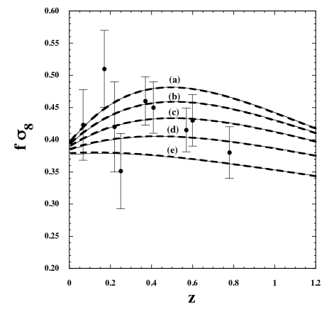
Figure 3: Evolution of $f\sigma_{8}$ versus $z$ for the models with $c_{s}^{2}=1$ and (a) $w=-1.2$, (b) $w=-1$, (c) $w=-0.8$, (d) $w=-0.6$, (e) $w=-0.4$, respectively. The solid lines correspond to the numerically integrated solutions, whereas the bald dashed lines are derived from the analytic estimation (52) with the 10-th order terms of $c_{n}$. We also show the current RSD data.

Let us first study constant $w$ models realized by either imperfect fluids or quintessence. Unless $c_{s}^{2}\ll 1$ the dark energy perturbation is negligible relative to the matter perturbation, so that the approximate equation (25) is sufficiently accurate. Since $w_{n}=0$ ($n\geq 1$), the coefficients $c_{n}$ and $\Omega_{x}$ are given, respectively, by

$$c_{n}=\alpha_{n}=\frac{(-1)^{n}}{n!}(\gamma-1)(\gamma-2)\cdots(\gamma-n)\,,\qquad\Omega_{x}=\frac{\Omega_{x0}(1+z)^{3w_{0}}}{1-\Omega_{x0}+\Omega_{x0}(1+z)^{3w_{0}}}\,.$$ (54)

For the growth index (42) we take into account the terms up to 2-nd order with respect to $\Omega_{x}$, i.e.,

$$\gamma=\frac{3(1-w_{0})}{5-6w_{0}}+\frac{3}{2}\frac{(1-w_{0})(2-3w_{0})}{(5-6w_{0})^{2}(5-12w_{0})}\Omega_{x}+\frac{(w_{0}-1)(3w_{0}-2)(324w_{0}^{2}-420w_{0}+97)}{4(5-6w_{0})^{3}(5-12w_{0})(5-18w_{0})}\Omega_{x}^{2}\,.$$ (55)

Recall that the terms higher than 2-nd order in $\gamma$ are negligibly small. Then $f\sigma_{8}$ is analytically known from Eq. (52) just by specifying the values of $\sigma_{8}(z=0)$, $\Omega_{x0}$, and $w=w_{0}$.

In Fig. 2 we plot the evolution of $f\sigma_{8}$ obtained by the analytic estimation (52) for $w=-0.9$ and $c_{s}^{2}=1$. A number of different lines correspond to the solutions derived by taking into account the $c_{n}$ terms up to 1-st, 3-rd, and 7-th orders. As we pick up higher-order coefficients $c_{n}$ in Eq. (54), the solutions tend to approach the numerically integrated solution of $f\sigma_{8}$. In Fig. 2 we find that the solution up to 7-th order terms of $c_{n}$ can reproduce the full numerical result in good precision.

In Fig. 3 we show $f\sigma_{8}$ versus $z$ for five different values of $w$. In order to obtain a good convergence we pick up the $c_{n}$ terms up to 10-th order. Figure 3 shows that our analytic estimation (52) is sufficiently trustable to reproduce the numerically integrated solutions accurately. If we only pick up the terms inside $\gamma$ up to 1-st order with respect to $\Omega_{x}$, there is small difference of $f\sigma_{8}$ between the analytic estimation and the numerical solutions for $w\gtrsim-0.6$ (which occurs in the low redshift regime). Taking into account the 2-nd order term in Eq. (42), this difference gets smaller. Fig. 3 also displays the RSD data given in Table 1, which will be used to place observational constraints on $w$ in Sec. VI.

V.2 Tracking quintessence models

From Eq. (33), we see that all coefficients $w_{n}$’s ($n\geq 1$) in tracking models of quintessence are expressed in terms of the tracker equation of state $w_{0}=w_{(0)}$. In this case there are contributions to $c_{n}$ coming from the variation of $w$, i.e., non-zero values of $\beta_{n}$. Note that $\beta_{n}$’s depend only on $w_{(0)}$.

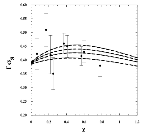
Figure 4: Evolution of $f\sigma_{8}$ versus $z$ for the tracking quintessence model characterized by the inverse power-law potential $V(\phi)=M^{4+p}\phi^{-p}$. From top to bottom the solid lines correspond to the numerically integrated solutions for $p=0.1,0.5,1,2$, respectively, whereas the bold dashed lines are derived from the analytic solution (52) with the 10-th order terms. The RSD data are the same as those given in Fig. 3.

For the tracking quintessence with the inverse power-law potential $V(\phi)=M^{4+p}\phi^{-p}$ ($p>0$), we compare the numerically integrated solutions of $f\sigma_{8}$ with those derived by the analytic expression (52). In Fig. 4 we show the evolution of $f\sigma_{8}$ for $p=0.1,0.5,1,2$ evaluated from (52) as well as the numerical solutions. In Eq. (52) we take into account the $c_{n}$’s up to 10-th order terms, whereas in the analytic expression of $\gamma$ in Eq. (42) the terms up to 2-nd order in $\Omega_{x}$ are included. For the evaluation of $\Omega_{x}$ the 1-st order solution (53) with $\Omega_{x0}=0.73$ is used. From Fig. 4 we find that the analytic solution (52) is accurate enough to reproduce the full numerical solution in high precisions. If we take into account the $c_{n}$’s up to the 3-rd order terms, for example, there is some difference between the analytic and numerical results. This difference tends to disappear by including the higher-order terms of $c_{n}$. While the terms up to 10-th order are taken into account in Fig. 4, the 7-th order solutions are sufficiently accurate.

While our analytic formula of $f\sigma_{8}$ is trustable, readers may think that 7-th order expansion of $c_{n}$ is not very convenient for practical purpose. However, using this analytic formula is simpler than solving the perturbation equations numerically for arbitrary initial conditions. If we take the latter approach, we need first to identify the present epoch (say, $0.7<\Omega_{x0}<0.73$) by solving the background equations from some redshift ($z=z_{i}$). Then the perturbation equations are solved with arbitrary initial values of $\sigma_{8}(z_{i})$ to find $f\sigma(z)$ for each $z$. On the other hand, with our analytic formula, the likelihood analysis in terms of 3 free parameters $w_{0}$, $\sigma_{8}(z=0)$, and $\Omega_{x0}$ can be done much easier even with the 7-th order expansion of $c_{n}$. We also would like to stress that our formula of $f\sigma_{8}(z)$ includes the free parameters $\sigma_{8}(z=0)$ and $\Omega_{x0}$ today, by which the joint analysis with other data (such as CMB) can be conveniently performed.

V.3 Thawing models

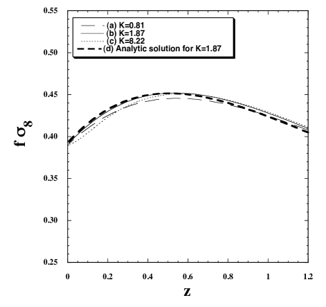
Figure 5: Evolution of $f\sigma_{8}$ versus $z$ for the freezing quintessence with the potential $V(\phi)=\Lambda^{4}[1+\cos(\phi/f)]$. The cases (a)-(c) correspond to the full numerical solutions with the model parameters (a) $K=0.81$, $w_{1}=0.17$, (b) $K=1.87$, $w_{1}=4.7\times 10^{-2}$, and (c) $K=8.22$, $w_{1}=3.6\times 10^{-6}$, respectively, whereas the case (d) is derived by the 10-th order analytic solution (52) for $K=1.87$, $w_{1}=4.7\times 10^{-2}$.

In thawing models of quintessence the field equation of state is given by Eq. (35). For larger $K$ the deviation of $w$ from $-1$ occurs at later times with a sharper transition. From Eq. (37) we find that the higher-order terms in $\Omega_{x}$ are not negligible for $K$ larger than the order of 1. In fact we have numerically confirmed that, for $K>{\cal O}(1)$, the expansion (37) does not accommodate the rapid transition of $w$ at late times unless the higher-order terms are fully taken into account. This property also holds for the evolution of $f\sigma_{8}$. Only when $K$ is smaller than the order of 1, the analytic estimation (52) can reproduce the full numerical solutions in good precision.

In Fig. 5 we plot the numerical evolution of $f\sigma_{8}$ for the potential $V(\phi)=\Lambda^{4}[1+\cos(\phi/f)]$ with three different values of $K$. Since $w$ is close to $-1$ in all these cases and the deviation from $w=-1$ occurs only at late times, the evolution of $f\sigma_{8}$ is not very different from each other for $K<10$. From this analysis, it is clear that, only when very accurate data of $f\sigma_{8}$ are available in the future, it will be possible to distinguish between the models with different values of $K$. In Fig. 5 we also show the analytic solution derived for $K=1.87$ and $w_{1}=4.7\times 10^{-2}$ as the bold dashed line (d). We take into account the $c_{n}$’s up to 10-th order to evaluate $f\sigma_{8}$ in Eq. (52). Compared to the full numerical solution labelled as (b), there is a small difference in the high-redshift regime. We confirm that this deviation tends to be smaller by involving the $c_{n}$’s higher than 10-th order. For $K<1$ the analytic estimation is more accurate even without including such higher-order terms.

VI Constraints from the current RSD data

In this section, we place observational bounds on two models of dark energy discussed in Secs. V.1 and V.2 by using the current RSD data presented in Table 1. For the today’s value of $\sigma_{8}$ we consider the prior obtained from observations of CMB, BAO, and Hubble constant measurement ($H_{0}$), i.e.,

$$\sigma_{8}(z=0)=0.816\pm 0.024\,.$$ (56)

Here and in what follows all the error bars correspond to the 68.3% confidence level (CL). Recall that we derived the analytic formula (52) under the approximation that the dark energy perturbation is neglected relative to the matter perturbation. For the validity of this approximation we put the prior $w<-0.1$.

VI.1 Constant $w$ models

For the models of constant $w$ the today’s matter density parameter constrained from SN Ia, CMB, BAO, and $H_{0}$ observations is Suzuki

$$\Omega_{m0}=0.272^{+0.013}_{-0.013}\,.$$ (57)

Under the priors (56) and (57) we estimate the best-fit to the set of parameters ${\mathbf{P}}\equiv(w,\sigma_{8}(z=0),\Omega_{m0})$ by evaluating the likelihood distribution function, ${\cal{L}}\propto e^{-\chi^{2}/2}$, with

$$\chi^{2}=\sum_{i=1}^{9}\left(\frac{f\sigma_{8,{\rm ob}}(z_{i})-f\sigma_{8,{\rm th}}(z_{i})}{\sigma_{i}}\right)^{2}\;.$$ (58)

Here $f\sigma_{8,{\rm ob}}(z_{i})$ ($i=1,\cdots,9$) are the 9 data displayed in Table 1 with the error bars $\sigma_{i}$, whereas $f\sigma_{8,{\rm th}}(z_{i})$ are the theoretical values derived from the analytic solution (52). For the evaluation of $f\sigma_{8,{\rm th}}(z_{i})$ we pick up the $c_{n}$’s up to 10-th order. For the growth index $\gamma$ the terms up to 2-nd order with respect to $\Omega_{x}$ are included in Eq. (42). For $\Omega_{x}$ we use the 1-st order solution (53). In tracking quintessence models analyzed in Sec. VI.2 we also take the same orders of expansions for $f\sigma_{8}$, $\gamma$, and $\Omega_{x}$.

We find that the best-fit model parameters are

$$w=-0.604\,,\qquad\sigma_{8}(z=0)=0.840\,,\qquad\Omega_{m0}=0.285\,,$$ (59)

with reduced $\chi^{2}_{r}=0.947$ ($\chi^{2}_{r}\equiv\chi^{2}_{\rm min}/\nu$, where $\nu$ stands for the degrees of freedom). At 68.3% CL, our analysis restricts the equation-of-state parameter to the interval

$$-1.245<w<-0.347\,,$$ (60)

whereas $\sigma_{8}(z=0)$ and $\Omega_{m0}$ are unconstrained by current data even assuming the priors (56) and (57). Although the current bounds on $w$ are weaker than those arising from background tests (see, e.g., Refs. Komatsu ; Suzuki ), we expect that upcoming RSD data from ongoing and planned galaxy redshift surveys can improve this situation in the near future.

VI.2 Tracking quintessence models

For the tracking quintessence models in which the equation of state is given by Eq. (32) we also carry out the likelihood analysis by using the analytic solution (52) of $f\sigma_{8}$ as well as the expressions for $\gamma$ and $\Omega_{x}$ given in Eqs. (42) and (53) respectively. While the equation of state (32) is derived for quintessence, we do not impose the prior $w_{(0)}>-1$ for generality. For this kind of models, a joint analysis involving current SN Ia, CMB, and BAO gives the following bound on the matter density parameter CDT :

$$0.273<\Omega_{m0}<0.293\,,$$ (61)

which is used in our analysis as a prior for $\Omega_{m0}$. The best-fit model parameters are found to be

$$w_{(0)}=-0.461\,,\qquad\sigma_{8}(z=0)=0.840\,,\qquad\Omega_{m0}=0.293\,,$$ (62)

with $\chi^{2}_{r}=0.923$. At 68.3% CL, we found

$$-1.288<w_{(0)}<-0.214\,,$$ (63)

whereas the parameters $\sigma_{8}(z=0)$ and $\Omega_{m0}$ are again unconstrained in the regions of (56) and (61). As expected, the bounds on $w_{(0)}$ are weaker than those obtained in constant $w$ models [Eq. (60)]. We note that in tracking models the equation of state decreases at late times, which is accompanied by the decrease of $f\sigma_{8}$. Compared to constant $w$ models, this allows the possibility to fit the data better even for larger values of $w$ during the matter era.

VII Conclusions

In this paper we have provided an analytic formula of $f\sigma_{8}$ for dynamical dark energy models in the framework of GR. This was derived by using the approximate matter perturbation equation (25), which is trustable as long as the contribution of the dark energy perturbation to the gravitational potential is negligible relative to that of the matter perturbation. Our formula of $f\sigma_{8}$ can be applied to many dark energy models including imperfect fluids, quintessence, and k-essence in which the sound speed squared $c_{s}^{2}$ is not very close to 0.

Our derivation of $f\sigma_{8}$ is based on the expansion of $w$ with respect to the dark energy density parameter $\Omega_{x}$, i.e., $w=w_{0}+\sum_{n=1}w_{n}(\Omega_{x})^{n}$. The growth rate $f=\delta_{m}^{\prime}/\delta_{m}$ of matter perturbations is parametrized by the growth index $\gamma$, as $f=(1-\Omega_{x})^{\gamma}$. We expanded $\gamma$ in terms of $\Omega_{x}$ up to 2-nd order terms. Since $\gamma$ is dominated by the term $\gamma_{0}=3(1-w_{0})/(5-6w_{0})$, it is a good approximation to treat $\gamma$ as a constant for the derivation of the integrated solution of $\delta_{m}$. The $c_{n}$’s in Eq. (52) are given by Eq. (47), where $\alpha_{n}$ and $\beta_{n}$ appear as the coefficients of the expansion of the terms $(1-\Omega_{x})^{\gamma-1}$ and $1/w$ respectively. For the density parameter $\Omega_{x}$, the 1-st order solution (53) is usually sufficient to obtain accurate analytic solutions of $f\sigma_{8}$.

In Sec. V we have studied the validity of the analytic formula (52) in concrete models of dark energy. For constant $w$ models in which $c_{n}$ and $\Omega_{x}$ are given by Eq. (54), the analytic solution up to 7-th order terms of $c_{n}$ reproduces the numerically integrated solutions with good precision. This property also holds for tracking quintessence models where the evolution of $w$ is given by Eq. (33). In thawing quintessence and k-essence models, where $w$ is given by Eq. (35), the formula (52) can be trustable for $K\lesssim 1$, but for $K$ larger than the order of 1, we need to fully take into account the higher-order terms of $c_{n}$ to have good convergence of $f\sigma_{8}$.

In Sec. VI we have discussed observational constraints on two different dark energy models by using the current RSD data. In both constant $w$ and tracking quintessence models the analytic solution (52) includes the three parameters $\sigma_{8}(z=0)$, $\Omega_{m0}$, and $w$ (or $w_{(0)}$). Under the priors on $\sigma_{8}(z=0)$ and $\Omega_{m0}$ constrained by SN Ia, CMB, BAO, and $H_{0}$ measurements, we derived the bounds $-1.245<w<-0.347$ (68 % CL) for constant $w$ models and $-1.288<w_{(0)}<-0.214$ (68 % CL) for tracking quintessence models. Although the upper bounds on the dark energy equation of state are still weak with current data, we expect to obtain more precise data from ongoing surveys or near-future projects such as Subaru/FMOS, HETDEX, and J-PAS. Our analytic formula of $f\sigma_{8}$ will be useful to place tighter bounds on dynamical dark energy models in the future.

So far, observational bounds on $f\sigma_{8}$ (listed in Table 1) have been derived in the standard cosmological scenario without taking into account additional effects such as a possible coupling between dark matter and dark energy, irrotational flow, and so on. Reflecting this observational status, we did not assume any non-standard picture to estimate the theoretical values of $f\sigma_{8}$. However, if the standard cosmological scenario does not match with future high-precision data very well, it may be necessary to include non-standard effects mentioned above as a next step. We leave the theoretical estimation of such effects for future work.

References

- (1) A. G. Riess et al. [Supernova Search Team Collaboration], Astron. J. 116, 1009 (1998); S. Perlmutter et al. [Supernova Cosmology Project Collaboration], Astrophys. J. 517, 565 (1999).
- (2) D. N. Spergel et al. [WMAP Collaboration], Astrophys. J. Suppl. 148, 175 (2003).
- (3) E. Komatsu et al. [WMAP Collaboration], Astrophys. J. Suppl. 192, 18 (2011).
- (4) D. J. Eisenstein et al. [SDSS Collaboration], of SDSS luminous red galaxies,” Astrophys. J. 633, 560 (2005); W. J. Percival et al. [SDSS Collaboration], Mon. Not. Roy. Astron. Soc. 401, 2148 (2010).
- (5) S. Weinberg, Rev. Mod. Phys. 61, 1 (1989).
- (6) V. Sahni and A. A. Starobinsky, Int. J. Mod. Phys. D 9, 373 (2000).
- (7) S. M. Carroll, Living Rev. Rel. 4, 1 (2001); T. Padmanabhan, Phys. Rept. 380, 235 (2003); P. J. E. Peebles and B. Ratra, Rev. Mod. Phys. 75, 559 (2003); E. J. Copeland, M. Sami and S. Tsujikawa, Int. J. Mod. Phys. D 15, 1753 (2006); T. P. Sotiriou and V. Faraoni, Rev. Mod. Phys. 82, 451 (2010); A. De Felice and S. Tsujikawa, Living Rev. Rel. 13, 3 (2010); S. Tsujikawa, Lect. Notes Phys. 800, 99 (2010); arXiv:1004.1493 [astro-ph.CO].
- (8) N. Suzuki et al., Astrophys. J. 746, 85 (2012).
- (9) C. Blake et al., Mon. Not. Roy. Astron. Soc. 418, 1707 (2011).
- (10) L. Anderson et al., arXiv:1203.6594 [astro-ph.CO].
- (11) A. De Felice, S. Nesseris and S. Tsujikawa, JCAP 1205, 029 (2012).
- (12) Y. Fujii, Phys. Rev. D 26, 2580 (1982); L. H. Ford, Phys. Rev. D 35, 2339 (1987); C. Wetterich, Nucl. Phys B. 302, 668 (1988); T. Chiba, N. Sugiyama and T. Nakamura, Mon. Not. Roy. Astron. Soc. 289, L5 (1997); P. G. Ferreira and M. Joyce, Phys. Rev. Lett. 79, 4740 (1997); R. R. Caldwell, R. Dave and P. J. Steinhardt, Phys. Rev. Lett. 80, 1582 (1998).
- (13) C. Armendariz-Picon, T. Damour and V. F. Mukhanov, Phys. Lett. B 458, 209 (1999).
- (14) T. Chiba, T. Okabe and M. Yamaguchi, Phys. Rev. D62, 023511 (2000); C. Armendariz-Picon, V. F. Mukhanov and P. J. Steinhardt, Phys. Rev. Lett. 85, 4438-4441 (2000).
- (15) S. Capozziello, Int. J. Mod. Phys. D 11, 483 (2002); S. Capozziello, S. Carloni and A. Troisi, Recent Res. Dev. Astron. Astrophys. 1, 625 (2003); S. M. Carroll, V. Duvvuri, M. Trodden and M. S. Turner, Phys. Rev. D 70, 043528 (2004); L. Amendola, R. Gannouji, D. Polarski and S. Tsujikawa, Phys. Rev. D 75, 083504 (2007); L. Amendola and S. Tsujikawa, Phys. Lett. B 660, 125 (2008); W. Hu and I. Sawicki, Phys. Rev. D 76, 064004 (2007); A. A. Starobinsky, JETP Lett. 86, 157 (2007); S. A. Appleby and R. A. Battye, Phys. Lett. B 654, 7 (2007); S. Tsujikawa, Phys. Rev. D 77, 023507 (2008); E. V. Linder, Phys. Rev. D 80, 123528 (2009); M. Campista, B. Santos, J. Santos and J. S. Alcaniz, Phys. Lett. B 699, 320 (2011); B. Santos, M. Campista, J. Santos and J. S. Alcaniz, arXiv:1207.2478 [astro-ph.CO].
- (16) M. Tegmark et al. [SDSS Collaboration], Phys. Rev. D 69, 103501 (2004); U. Seljak et al. [SDSS Collaboration], Phys. Rev. D 71, 103515 (2005); M. Tegmark et al. [SDSS Collaboration], Phys. Rev. D 74, 123507 (2006).
- (17) N. Kaiser, Mon. Not. Roy. Astron. Soc. 227, 1 (1987).
- (18) M. Tegmark et al. [SDSS Collaboration], Astrophys. J. 606, 702 (2004).
- (19) W. J. Percival et al. [The 2dFGRS Collaboration], Mon. Not. Roy. Astron. Soc. 353, 1201 (2004).
- (20) C. Di Porto and L. Amendola, Phys. Rev. D 77, 083508 (2008).
- (21) L. Guzzo et al., Nature 451, 541 (2008).
- (22) S. Nesseris and L. Perivolaropoulos, Phys. Rev. D 77, 023504 (2008).
- (23) U. Alam, V. Sahni and A. A. Starobinsky, Astrophys. J. 704, 1086 (2009).
- (24) C. Blake et al., Mon. Not. Roy. Astron. Soc. 415, 2876 (2011).
- (25) L. Samushia, W. J. Percival and A. Raccanelli, Mon. Not. Roy. Astron. Soc. 420, 2102 (2012).
- (26) B. A. Reid et al., arXiv:1203.6641 [astro-ph.CO].
- (27) F. Beutler et al., arXiv:1204.4725 [astro-ph.CO].
- (28) E. Jennings, C. M. Baugh, B. Li, G. -B. Zhao and K. Koyama, arXiv:1205.2698 [astro-ph.CO].
- (29) D. Rapetti, C. Blake, S. W. Allen, A. Mantz, D. Parkinson and F. Beutler, arXiv:1205.4679 [astro-ph.CO].
- (30) L. Samushia et al., arXiv:1206.5309 [astro-ph.CO].
- (31) S. A. Appleby and E. V. Linder, JCAP 1208, 026 (2012).
- (32) H. Okada, T. Totani and S. Tsujikawa, arXiv:1208.4681 [astro-ph.CO].
- (33) S. M. Carroll, I. Sawicki, A. Silvestri and M. Trodden, New J. Phys. 8, 323 (2006); R. Bean, D. Bernat, L. Pogosian, A. Silvestri and M. Trodden, Phys. Rev. D 75, 064020 (2007); S. Tsujikawa, Phys. Rev. D 76, 023514 (2007); L. Pogosian and A. Silvestri, Phys. Rev. D 77, 023503 (2008); S. Tsujikawa, R. Gannouji, B. Moraes and D. Polarski, Phys. Rev. D 80, 084044 (2009).
- (34) A. De Felice, R. Kase and S. Tsujikawa, Phys. Rev. D 83, 043515 (2011).
- (35) A. De Felice and S. Tsujikawa, JCAP 1203, 025 (2012).
- (36) I. Zlatev, L. M. Wang and P. J. Steinhardt, Phys. Rev. Lett. 82, 896 (1999); P. J. Steinhardt, L. -M. Wang and I. Zlatev, Phys. Rev. D 59, 123504 (1999).
- (37) J. M. Bardeen, Phys. Rev. D 22, 1882 (1980).
- (38) H. Kodama and M. Sasaki, Prog. Theor. Phys. Suppl. 78, 1 (1984).
- (39) R. Bean and O. Dore, Phys. Rev. D 69, 083503 (2004).
- (40) D. Sapone, M. Kunz and L. Amendola, Phys. Rev. D 82, 103535 (2010).
- (41) L. Amendola and S. Tsujikawa, Dark energy–Theory and Observations, Cambridge University Press (2010).
- (42) B. A. Bassett, S. Tsujikawa and D. Wands, Rev. Mod. Phys. 78, 537 (2006).
- (43) J. Garriga and V. F. Mukhanov, Phys. Lett. B 458, 219 (1999).
- (44) M. Tegmark et al. [SDSS Collaboration], Phys. Rev. D 74, 123507 (2006).
- (45) Y. -S. Song and W. J. Percival, JCAP 0910, 004 (2009).
- (46) M. White, Y. -S. Song and W. J. Percival, Mon. Not. Roy. Astron. Soc. 397, 1348 (2008).
- (47) G. Ballesteros and A. Riotto, Phys. Lett. B 668, 171 (2008).
- (48) V. Sahni, T. D. Saini, A. A. Starobinsky and U. Alam, JETP Lett. 77, 201 (2003).
- (49) V. Sahni and A. Starobinsky, Int. J. Mod. Phys. D 15, 2105 (2006).
- (50) R. R. Caldwell and E. V. Linder, Phys. Rev. Lett. 95, 141301 (2005).
- (51) P. J. E. Peebles and B. Ratra, Astrophys. J. 325, L17 (1988); B. Ratra and J. Peebles, Phys. Rev D 37, 3406 (1988).
- (52) T. Chiba, Phys. Rev. D 81, 023515 (2010).
- (53) J. A. Frieman, C. T. Hill, A. Stebbins and I. Waga, Phys. Rev. Lett. 75, 2077 (1995).
- (54) S. Dutta and R. J. Scherrer, Phys. Rev. D 78, 123525 (2008).
- (55) R. J. Scherrer and A. A. Sen, Phys. Rev. D 77, 083515 (2008).
- (56) T. Chiba, S. Dutta and R. J. Scherrer, Phys. Rev. D 80, 043517 (2009).
- (57) F. Piazza and S. Tsujikawa, JCAP 0407, 004 (2004).
- (58) N. Arkani-Hamed, H. -C. Cheng, M. A. Luty and S. Mukohyama, JHEP 0405, 074 (2004).
- (59) L. -M. Wang and P. J. Steinhardt, Astrophys. J. 508, 483 (1998).
- (60) P. J. E. Peebles, Large-Scale Structure of the Universe, Princeton University Press (1980).
- (61) Y. Gong, M. Ishak and A. Wang, Phys. Rev. D 80, 023002 (2009).
- (62) E. V. Linder, Phys. Rev. D 72, 043529 (2005); E. V. Linder and R. N. Cahn, Astropart. Phys. 28, 481 (2007).
- (63) T. Chiba, A. De Felice, and S. Tsujikawa, arXiv:1210.3859 [astro-ph.CO].