Application of the BDEs Method to One Problem of Free Turbulence

Application of the $\boldsymbol{B}$-Determining Equations Method
to One Problem of Free Turbulence

Oleg V. KAPTSOV and Alexey V. SCHMIDT

O.V. Kaptsov and A.V. Schmidt

Institute of Computational Modeling SB RAS, Akademgorodok, Krasnoyarsk, 660036, Russia kaptsov@icm.krasn.ru, schmidt@icm.krasn.ru

Received May 17, 2012, in final form October 04, 2012; Published online October 16, 2012

A three-dimensional model of the far turbulent wake behind a self-propelled body in a passively stratified medium is considered. The model is reduced to a system of ordinary differential equations by a similarity reduction and the $B$-determining equations method. The system of ordinary differential equations satisfying natural boundary conditions is solved numerically. The solutions obtained here are in close agreement with experimental data.

turbulence; far turbulent wake; $B$-determining equations method

76M60; 76F60

1 Introduction

Most flows occurring in nature and engineering practice are turbulent (see, e.g., [10, 20, 22]). Semiempirical models of turbulence are widely used in the modeling of turbulent flows [16, 21, 27]. However, there are only a few analytical results on such models (see, e.g., [2, 11]).

The far turbulent wake behind an axisymmetric body in a stratified medium is an example of a free shear flow. Sufficiently complete experimental data on the dynamics of turbulent wakes generated by moving bodies in stratified fluids were obtained by Lin and Pao [17].

The far turbulent wake behind an axisymmetric towed body in a linearly stratified medium was numerically simulated in [9]. Chernykh et al. [6] carried out the numerical simulation of the dynamics of turbulent wakes in a stable stratified medium based on hierarchy of second order closure models. Calculation results obtained in [6, 9] are in close agreement with experimental data [17].

Similarity solutions for several turbulence models were constructed in [7, 13, 14, 15]. In the current paper we consider three-dimensional semiempirical model of the far turbulent wake behind an axisymmetrical self-propelled body in a passively stratified medium (see [6, 4, 25] and the references therein).

This paper is organized as follows. In Section 3 we determine the most general continuous classical symmetry group of the model and obtain the similarity reduction of the model. In Section 4 we use the $B$-determining equations (BDEs) method [1, 12] to transform the reduced system into a system of ordinary differential equations (ODEs).

In the last section, we consider a boundary value problem for the system of ODEs. We use the modified shooting method and the asymptotic expansion of the solution in the vicinity of the singular point to solve this problem. Finally, computational results are given.

2 Model

The following three-dimensional semiempirical model of turbulence was constructed in [4, 6, 25] to calculate characteristics of the far turbulent wake behind an axisymmetric self-propelled body in a passively stratified medium:

$$U_{0}\frac{\partial e}{\partial x}=\frac{\partial}{\partial y}C_{e}\frac{e^{2}}{\varepsilon}\frac{\partial e}{\partial y}+\frac{\partial}{\partial z}C_{e}\frac{e^{2}}{\varepsilon}\frac{\partial e}{\partial z}-\varepsilon,$$ (1)

$$U_{0}\frac{\partial\varepsilon}{\partial x}=\frac{\partial}{\partial y}C_{\varepsilon}\frac{e^{2}}{\varepsilon}\frac{\partial\varepsilon}{\partial y}+\frac{\partial}{\partial z}C_{\varepsilon}\frac{e^{2}}{\varepsilon}\frac{\partial\varepsilon}{\partial z}-{C_{\varepsilon}}_{2}\frac{\varepsilon^{2}}{e},$$ (2)

$$U_{0}\frac{\partial\langle\rho_{1}\rangle}{\partial x}=\frac{\partial}{\partial y}C_{\rho}\frac{e^{2}}{\varepsilon}\frac{\partial\langle\rho_{1}\rangle}{\partial y}+\frac{\partial}{\partial z}C_{\rho}\frac{e^{2}}{\varepsilon}\frac{\partial\langle\rho_{1}\rangle}{\partial z}-\frac{\partial}{\partial z}C_{\rho}\frac{e^{2}}{\varepsilon},$$ (3)

$$U_{0}\frac{\partial\langle\rho^{\prime 2}\rangle}{\partial x}=\frac{\partial}{\partial y}{C_{1}}_{\rho}\frac{e^{2}}{\varepsilon}\frac{\partial\langle\rho^{\prime 2}\rangle}{\partial y}+\frac{\partial}{\partial z}{C_{1}}_{\rho}\frac{e^{2}}{\varepsilon}\frac{\partial\langle\rho^{\prime 2}\rangle}{\partial z}+2C_{\rho}\frac{e^{2}}{\varepsilon}{\frac{\partial\langle\rho_{1}\rangle}{\partial y}}^{2}$$

$$\hphantom{U_{0}\frac{\partial\langle\rho^{\prime 2}\rangle}{\partial x}=}{}+2C_{\rho}\frac{e^{2}}{\varepsilon}\left(\frac{\partial\langle\rho_{1}\rangle}{\partial z}-1\right)^{2}-C_{T}\frac{\langle\rho^{\prime 2}\rangle\varepsilon}{e},$$ (4)

where $e$ is the turbulent kinetic energy, $\varepsilon$ is the kinetic energy dissipation rate, $\langle\rho_{1}\rangle$ is the averaged density defect, and $\langle\rho^{\prime 2}\rangle$ is the density fluctuation variance. All the unknown functions depend on $x$, $y$, and $z$. The quantities $C_{e}=0.136$, $C_{\varepsilon}=C_{e}/\delta$, $\delta=1.3$, ${C_{\varepsilon}}_{2}=1.92$, $C_{\rho}=0.208$, ${C_{1}}_{\rho}=0.087$, $C_{T}=1.25$ are generally accepted empirical constant [8, 21]. $U_{0}$ is the free stream velocity. The marching variable $x$ in the equations (1)–(4) acts as time.

This model is based on the three-dimensional parabolized system of averaged Navier–Stokes equations in the Oberbeck–Boussinesq approximation (see [5, 26])

$$U_{0}\frac{\partial U_{d}}{\partial x}+V\frac{\partial U_{d}}{\partial y}+W\frac{\partial U_{d}}{\partial z}=\frac{\partial}{\partial y}\langle u^{\prime}v^{\prime}\rangle+\frac{\partial}{\partial z}\langle u^{\prime}w^{\prime}\rangle,$$ (5)

$$U_{0}\frac{\partial V}{\partial x}+V\frac{\partial V}{\partial y}+W\frac{\partial V}{\partial z}=-\frac{1}{\rho_{0}}\frac{\partial\langle p_{1}\rangle}{\partial y}-\frac{\partial}{\partial y}\langle v^{\prime 2}\rangle-\frac{\partial}{\partial z}\langle v^{\prime}w^{\prime}\rangle,$$ (6)

$$U_{0}\frac{\partial W}{\partial x}+V\frac{\partial W}{\partial y}+W\frac{\partial W}{\partial z}=-\frac{1}{\rho_{0}}\frac{\partial\langle p_{1}\rangle}{\partial z}-\frac{\partial}{\partial y}\langle v^{\prime}w^{\prime}\rangle-\frac{\partial}{\partial z}\langle w^{\prime 2}\rangle-g\frac{\langle\rho_{1}\rangle}{\rho_{0}},$$ (7)

$$U_{0}\frac{\partial\langle\rho_{1}\rangle}{\partial x}+V\frac{\partial\langle\rho_{1}\rangle}{\partial y}+W\frac{\partial\langle\rho_{1}\rangle}{\partial z}+W\frac{\partial\rho_{s}}{\partial z}=-\frac{\partial}{\partial y}\langle v^{\prime}\rho^{\prime}\rangle-\frac{\partial}{\partial z}\langle w^{\prime}\rho^{\prime}\rangle,$$ (8)

$$\frac{\partial V}{\partial y}+\frac{\partial W}{\partial z}=\frac{\partial U_{d}}{\partial x},$$ (9)

where $U_{d}=U_{0}-U$ is the defect of the averaged longitudinal velocity component; $U$, $V$ and $W$ are the mean flow velocity component along $x$-, $y$- and $z$-axes, respectively; $\langle p_{1}\rangle$ is the deviation from the hydrostatic pressure due to stratification $\rho_{s}(z)$; $g$ is the gravity acceleration; $\langle\rho_{1}\rangle$ is the averaged density defect: $\rho_{1}=\rho-\rho_{s}$; $\rho_{s}=\rho_{s}(z)$ is the undisturbed fluid density assumed to be linear: $\rho_{s}(z)=\rho_{0}(1-az)$, $a>0$ is a constant; the prime indicates the pulsating components; $\langle\ \rangle$ indicates averaging.

In [9, 26] the Reynolds stress tensor components $\langle u_{i}^{\prime}u_{j}^{\prime}\rangle$, the turbulent flows $\langle u^{\prime}_{i}\rho^{\prime}\rangle$, and the density fluctuation variance $\langle\rho^{\prime 2}\rangle$ are defined by the algebraic relations [21]. Since the flow in the far turbulent wake is considered, these relations are simplified as follows

$$\langle u^{\prime}v^{\prime}\rangle=\frac{1-c_{2}}{c_{1}}\frac{e\langle v^{\prime 2}\rangle}{\varepsilon}\frac{\partial U_{d}}{\partial y}=K_{y}\frac{\partial U_{d}}{\partial y},$$ (10)

$$\langle u^{\prime}w^{\prime}\rangle=\frac{(1-c_{2})e\langle w^{\prime 2}\rangle-\displaystyle\frac{\mathstrut(1-c_{3})(1-c_{2T})}{c_{1T}}\frac{g}{\rho_{0}}\frac{e^{2}}{\varepsilon}\langle w^{\prime}\rho^{\prime}\rangle}{c_{1}\varepsilon\left(1-\displaystyle\frac{\mathstrut 1-c_{3}}{c_{1}c_{1T}}\frac{g}{\rho_{0}}\frac{e^{2}}{\varepsilon^{2}}\frac{\partial\langle\rho\rangle}{\partial z}\right)}\frac{\partial U_{d}}{\partial z}=K_{z}\frac{\partial U_{d}}{\partial z},$$ (11)

$$\langle v^{\prime 2}\rangle=\frac{2}{3}e\left(1-\frac{1-c_{2}}{c_{1}}\frac{P}{\varepsilon}-\frac{1-c_{2}}{c_{1}}\frac{G}{\varepsilon}\right),$$ (12)

$$\langle w^{\prime 2}\rangle=\frac{2}{3}e\left(1-\frac{1-c_{2}}{c_{1}}\frac{P}{\varepsilon}+2\frac{1-c_{2}}{c_{1}}\frac{G}{\varepsilon}\right),$$ (13)

$$\langle\rho^{\prime 2}\rangle=\frac{2}{c_{T}}\frac{e}{\varepsilon}\langle w^{\prime}\rho^{\prime}\rangle\frac{\partial\langle\rho\rangle}{\partial z},$$ (14)

$$-\langle u^{\prime}\rho^{\prime}\rangle=\frac{1}{c_{1T}}\frac{e}{\varepsilon}\left(\langle u^{\prime}w^{\prime}\rangle\frac{\partial\langle\rho\rangle}{\partial z}+(1-c_{2T})\langle w^{\prime}\rho^{\prime}\rangle\frac{\partial\langle U\rangle}{\partial z}\right),$$ (15)

$$-\langle v^{\prime}\rho^{\prime}\rangle=\frac{1}{c_{1T}}\frac{e}{\varepsilon}\langle v^{\prime 2}\rangle\frac{\partial\langle\rho\rangle}{\partial y}=K_{\rho y}\frac{\partial\langle\rho\rangle}{\partial y},$$ (16)

$$-\langle w^{\prime}\rho^{\prime}\rangle=\frac{e}{c_{1T}\varepsilon}\left(\langle w^{\prime 2}\rangle\frac{\partial\langle\rho\rangle}{\partial z}+(1-c_{2T})\frac{g}{\rho_{0}}\langle\rho^{\prime 2}\rangle\right)$$

$$\hphantom{-\langle w^{\prime}\rho^{\prime}\rangle}{}=\frac{e\langle w^{\prime 2}\rangle}{c_{1T}\varepsilon\left(1-2\displaystyle\frac{\mathstrut 1-c_{2T}}{c_{1T}c_{2T}}\frac{g}{\rho_{0}}\frac{e^{2}}{\varepsilon^{2}}\frac{\partial\langle\rho\rangle}{\partial z}\right)}\frac{\partial\langle\rho\rangle}{\partial z}=K_{\rho z}\frac{\partial\langle\rho\rangle}{\partial z},$$ (17)

$$P=\left(\langle u^{\prime}v^{\prime}\rangle\frac{\partial U_{d}}{\partial y}+\langle u^{\prime}w^{\prime}\rangle\frac{\partial U_{d}}{\partial z}\right),$$ (18)

$$G=-\frac{1}{\rho_{0}}\langle w^{\prime}\rho^{\prime}\rangle g.$$ (19)

Differential transport equations [21] are used in [4, 6, 25] to determine the kinetic turbulent energy $e$, the kinetic energy dissipation rate $\varepsilon$, and the shear Reynolds stress $v^{\prime}w^{\prime}$:

$$U_{0}\frac{\partial e}{\partial x}+V\frac{\partial e}{\partial y}+W\frac{\partial e}{\partial z}=\frac{\partial}{\partial y}K_{ey}\frac{\partial e}{\partial y}+\frac{\partial}{\partial z}K_{ez}\frac{\partial e}{\partial z}+P+G-\varepsilon,$$ (20)

$$U_{0}\frac{\partial\varepsilon}{\partial x}+V\frac{\partial\varepsilon}{\partial y}+W\frac{\partial\varepsilon}{\partial z}=\frac{\partial}{\partial y}K_{\varepsilon y}\frac{\partial\varepsilon}{\partial y}+\frac{\partial}{\partial z}K_{\varepsilon z}\frac{\partial\varepsilon}{\partial z}+c_{\varepsilon 1}\frac{\varepsilon}{e}(P+G)-c_{\varepsilon 2}\frac{\varepsilon^{2}}{e},$$ (21)

$$U_{0}\frac{\partial\langle v^{\prime}w^{\prime}\rangle}{\partial x}+V\frac{\partial\langle v^{\prime}w^{\prime}\rangle}{\partial y}+W\frac{\partial\langle v^{\prime}w^{\prime}\rangle}{\partial z}=\frac{\partial}{\partial y}K_{ey}\frac{\partial\langle v^{\prime}w^{\prime}\rangle}{\partial y}+\frac{\partial}{\partial z}K_{ez}\frac{\partial\langle v^{\prime}w^{\prime}\rangle}{\partial z}$$

$$\qquad{}+(c_{2}-1)\left(\langle v^{\prime 2}\rangle\frac{\partial W}{\partial y}+\langle w^{\prime 2}\rangle\frac{\partial V}{\partial z}\right)+(1-c_{3})\frac{g}{\rho_{0}}\langle v^{\prime}\rho^{\prime}\rangle-c_{1}\frac{\varepsilon}{e}\langle v^{\prime}w^{\prime}\rangle.$$ (22)

The turbulent viscosity coefficients in these equations are $K_{ey}=K_{y}$, $K_{ez}=K_{z}$, $K_{\varepsilon y}=K_{ey}/\delta$, $K_{\varepsilon z}=K_{ez}/\delta$. The model (1)–(4) is an analogue of the equations (5)–(22) (for the diffusion approximation in a homogeneous fluid $V=0$, $W=0$, and $g=0$). In what follows, we assume that the free stream velocity $U_{0}$ equals unity.

3 Similarity solution

The infinitesimal symmetry group [18, 19] of the model (1)–(4) is spanned by the eight vector fields

$$X_{1}=\frac{\partial}{\partial x},\!\qquad X_{2}=\frac{\partial}{\partial y},\!\qquad X_{3}=\frac{\partial}{\partial z},\!\qquad X_{4}=\frac{\partial}{\partial\langle\rho_{1}\rangle},\!\qquad X_{5}=-z\frac{\partial}{\partial y}+y\frac{\partial}{\partial z}+y\frac{\partial}{\partial\langle\rho_{1}\rangle},$$

$$X_{6}=y\frac{\partial}{\partial y}+z\frac{\partial}{\partial z}+2e\frac{\partial}{\partial e}+2\varepsilon\frac{\partial}{\partial\varepsilon}+\langle\rho_{1}\rangle\frac{\partial}{\partial\langle\rho_{1}\rangle}+2\langle\rho^{\prime 2}\rangle\frac{\partial}{\partial\langle\rho^{\prime 2}\rangle},$$

$$X_{7}=x\frac{\partial}{\partial x}-2e\frac{\partial}{\partial e}-3\varepsilon\frac{\partial}{\partial\varepsilon},\qquad X_{8}=(\langle\rho_{1}\rangle-z)\frac{\partial}{\partial\langle\rho_{1}\rangle}+2\langle\rho^{\prime 2}\rangle\frac{\partial}{\partial\langle\rho^{\prime 2}\rangle}.$$

Available experimental data [10, 17] and numerical calculations [9, 20, 27] show that the flow in the far turbulent wake can be considered to be close to a self-similar flow. We therefore consider the linear combination of scaling vector fields $X_{6}$ and $X_{7}$

$$Z=x\frac{\partial}{\partial x}+\alpha y\frac{\partial}{\partial y}+\alpha z\frac{\partial}{\partial z}+2(\alpha-1)e\frac{\partial}{\partial e}+(2\alpha-3)\varepsilon\frac{\partial}{\partial\varepsilon}+\alpha\langle\rho_{1}\rangle\frac{\partial}{\partial\langle\rho_{1}\rangle}+2\alpha\langle\rho^{\prime 2}\rangle\frac{\partial}{\partial\langle\rho^{\prime 2}\rangle}.$$

The similarity variables associated with the infinitesimal generator $Z$ are

$$\xi=\frac{y}{x^{\alpha}},\quad\eta=\frac{z}{x^{\alpha}},\qquad e=x^{2\alpha-2}E(\xi,\eta),\qquad\varepsilon=x^{2\alpha-3}G(\xi,\eta),$$

$$\langle\rho_{1}\rangle=x^{\alpha}H(\xi,\eta),\qquad\langle\rho^{\prime 2}\rangle=x^{2\alpha}R(\xi,\eta),$$

where $E$, $G$, $H$, and $R$ are arbitrary functions. According to physical considerations (the influence of gravity is neglected in this problem), the functions $E$ and $G$ must be of the form

$$E(\xi,\eta)=E\Big{(}\sqrt{\xi^{2}+\eta^{2}}\Big{)},\qquad G(\xi,\eta)=G\Big{(}\sqrt{\xi^{2}+\eta^{2}}\Big{)}.$$ (23)

We obtain the reduced system by introducing similarity variables. Using (23) and changing to polar coordinates $\xi=r\cos\phi$, $\eta=r\sin\phi$ the reduced system becomes

$$C_{e}\frac{E}{G}\left(EE^{\prime\prime}+2E^{\prime 2}-\frac{E}{G}E^{\prime}G^{\prime}+\frac{E}{r}E^{\prime}\right)+\alpha rE^{\prime}+2(1-\alpha)E-G=0,$$ (24)

$$C_{\varepsilon}\frac{E}{G}\left(EG^{\prime\prime}-\frac{E}{G}G^{\prime 2}+2E^{\prime}G^{\prime}+\frac{E}{r}G^{\prime}\right)+\alpha rG^{\prime}+(3-2\alpha)G-{C_{\varepsilon}}_{2}\frac{G^{2}}{E}=0,$$ (25)

$$C_{\rho}\frac{E^{2}}{G}\left(H_{rr}+\frac{1}{r^{2}}H_{\phi\phi}\right)+\left(C_{\rho}\frac{E}{G}\left(2E^{\prime}-\frac{E}{G}G^{\prime}+\frac{E}{r}\right)+\alpha r\right)H_{r}-\alpha H$$

$$\qquad{}+C_{\rho}\frac{E}{G}\left(\frac{E}{G}G^{\prime}-2E^{\prime}\right)\sin\phi=0,$$ (26)

$${{C_{1}}_{\rho}}\frac{E^{2}}{G}\left(R_{rr}+\frac{1}{r^{2}}R_{\phi\phi}\right)+\left({{C_{1}}_{\rho}}\frac{E}{G}\left(\frac{E}{r}+2E^{\prime}-\frac{E}{G}G^{\prime}\right)+\alpha r\right)R_{r}-\left(C_{T}\frac{E}{G}+2\alpha\right)R$$

$$\qquad{}+2C_{\rho}\frac{E^{2}}{G}\left(H_{r}^{2}+\frac{1}{r^{2}}H_{\phi}^{2}\right)+2C_{\rho}\frac{E^{2}}{G}-4C_{\rho}\frac{E^{2}}{G}\left(H_{r}\sin\phi+H_{\phi}\frac{\cos\phi}{r}\right)=0,$$ (27)

where $E=E(r)$, $G=G(r)$, $H=H(r,\phi)$, and $R=R(r,\phi)$. Here, and throughout, subscripts denote derivatives, so $H_{r}=\partial H/\partial r$, etc.

Lie’s classical method do not provide solution of the reduced system agreed with experimental data. We therefore use the BDEs method.

4 BDEs method

The concept of BDEs of a system of partial differential equations (PDEs) was introduced in [1, 12]. Consider a scalar PDE

$$\Omega\big{(}{\bf{x}},u,u^{1},u^{2},\dots\big{)}=0,$$ (28)

where ${\bf{x}}=(x_{1},x_{2},\dots,x_{n})$ denotes $n$ independent variables, $u$ denotes the dependent variable, and

$$u_{k}=\frac{\partial u^{k}}{\partial x_{i_{1}}\partial x_{i_{2}}\cdots\partial x_{i_{k}}}$$

denotes the set of coordinates corresponding to all $k$-th order partial derivatives of $u$ with respect to ${\bf{x}}$. In the BDEs method, an extension of the classical symmetry determining relations is made by incorporating an additional factor $B({\bf{x}},u,u^{1},u^{2},\dots)$. For a scalar PDE (28), BDE is

$$h\frac{\partial\Omega}{\partial u}+\sum_{|\alpha|\geq 1}D^{\alpha}(h)\frac{\partial\Omega}{\partial u_{\alpha}}+Bh|_{\Omega=0}=0,$$ (29)

where $h$ is a function of ${\bf{x}},u,u^{1},u^{2},\dots$; $D^{\alpha}=D^{\alpha_{1}}_{x_{1}}\cdots D^{\alpha_{n}}_{x_{n}}$, $D_{x_{i}}$ is the total $x_{i}$ derivative; $\alpha$ is a multi-index. Equality (29) must hold for all solutions of (28).

Now we use the BDEs method to reduce (26) and (27) to some ODEs. Consider more general equation than (26)

$$H_{\phi\phi}+r^{2}H_{rr}+A(r)H_{r}+B(r)H+C(r)\sin\phi=0,$$ (30)

where $A(r)$, $B(r)$, and $C(r)$ are arbitrary functions. BDE corresponding to (30) is

$$D_{\phi}^{2}h+r^{2}D_{r}^{2}h+b_{1}(r,\phi)D_{r}h+b_{2}(r,\phi)h=0.$$ (31)

Here, and throughout $D_{\phi}$, $D_{r}$ are the operators of total differentiation with respect to $\phi$ and $r$. The function $h$ may depend on $r$, $\phi$, $H$ and derivatives of $H$. The functions $b_{1}(r,\phi)$ and $b_{2}(r,\phi)$ are to be determined together with the function $h$. Note that if we let in (31)

$$b_{1}(r,\phi)=A(r),\qquad b_{2}(r,\phi)=B(r),$$

we obtain the classical determining equation [18, 19].

For simplicity, we assume that a solution of (31) is independent of $r$ and partial derivatives of $H$ with respect to $r$

$$h=H_{\phi\phi}+h_{1}\left(\phi,H,H_{\phi}\right).$$ (32)

Substituting (32) into (31) gives a polynomial equation for derivatives of the fourth order. This polynomial must identically vanish. We can express the derivatives $H_{rr\phi\phi}$, $H_{\phi\phi\phi\phi}$, $H_{r\phi\phi}$, $H_{\phi\phi\phi}$, and $H_{\phi\phi}$ using (30). The coefficient of $H_{rrr}$ implies $b_{1}(r,\phi)=A(r)$.

As a result, the left side of (31) is a polynomial in $H_{rr}$ and $H_{r\phi}$. Collecting similar terms we obtain

$$2\left(A(r)H_{r}+B(r)H+C(r)\sin\phi\right)h_{1_{H_{\phi}H_{\phi}}}-2H_{\phi}h_{1_{HH_{\phi}}}-2h_{1_{\phi H_{\phi}}}+B(r)-b_{2}(r,\phi)=0,$$

$$h_{1_{H_{\phi}H_{\phi}}}=0,\qquad h_{1_{HH_{\phi}}}=0.$$

Hence

$$h_{1}\left(\phi,H,H_{\phi}\right)=h_{2}(\phi)H_{\phi}+h_{3}(\phi,H),\qquad b_{2}(r,\phi)=B(r)-2h_{2}^{\prime}(\phi).$$

Substituting the functions $b_{1}$, $b_{2}$, and $h_{1}$ into the left side of (31) we obtain the polynomial with respect to $H_{r}$ and $H_{\phi}$. This polynomial must identically vanish. Collecting similar terms we have

$$(B(r)H+C(r)\sin\phi)h_{3_{H}}-h_{3_{\phi\phi}}+(2h_{2}^{\prime}-B(r))h_{3}+C(r)(h_{2}\cos\phi-\sin\phi)=0,$$

$$h_{3_{HH}}=0,\qquad 2h_{3_{\phi H}}+h_{2}^{\prime\prime}-2h_{2}^{\prime}h_{2}=0.$$

Thus,

$$h_{3}(\phi,H)=\left(\frac{1}{2}h_{2}^{2}-\frac{1}{2}h_{2}^{\prime}+h_{4}\right)H,\qquad h_{2}^{\prime}-h_{2}^{2}-2\cot\phi h_{2}+2(1-h_{4})=0,$$ (33)

where $h_{4}$ is an arbitrary constant.

Clearly, that the Riccati equation (33) has the partial solution

$$h_{2}=\tan\phi$$

for $h_{4}=1/2$.

Thus we find the solution of (31)

$$h=H_{\phi\phi}+H_{\phi}\tan\phi.$$

The corresponding differential constraint $h=0$ has the general solution

$$H=H_{1}(r)\sin\phi+H_{2}(r),$$ (34)

where $H_{1}$ and $H_{2}$ are arbitrary functions.

Next we use (34) and consider the equation (27) in more general form

$$R_{\phi\phi}+r^{2}R_{rr}+K(r)R_{r}+L(r)R+M(r)\sin^{2}\phi+N(r)\sin\phi+P(r)=0,$$ (35)

where $K(r)$, $L(r)$, $M(r)$, $N(r)$, and $P(r)$ are arbitrary functions. The BDEs method applied to the equation (35) gives rise to the following results:

$$N(r)=0,\qquad b_{1}(r,\phi)=K(r),\qquad b_{2}(r,\phi)=L(r)-8\sin^{-2}2\phi,$$

$$h=R_{\phi\phi}-2R_{\phi}\cot 2\phi.$$

Integrating differential constraint $h=0$ corresponding to the BDE solution (34), we find

$$R=R_{1}(r)\sin^{2}\phi+R_{2}(r),$$ (36)

where $R_{1}(r)$ and $R_{2}(r)$ are arbitrary functions. Using (34) and (36) we obtain the following corollary in terms of variables $x$, $y$, and $z$.

Corollary 4.1.

The following expressions for the unknown functions

$$e=x^{2\alpha-2}E\left(\frac{\sqrt{y^{2}+z^{2}}}{x^{\alpha}}\right),\qquad\varepsilon=x^{2\alpha-3}G\left(\frac{\sqrt{y^{2}+z^{2}}}{x^{\alpha}}\right),$$ (37)

$$\langle\rho_{1}\rangle=zH\left(\frac{\sqrt{y^{2}+z^{2}}}{x^{\alpha}}\right),\qquad\langle\rho^{\prime 2}\rangle=z^{2}R_{1}\left(\frac{\sqrt{y^{2}+z^{2}}}{x^{\alpha}}\right)+x^{2\alpha}R_{2}\left(\frac{\sqrt{y^{2}+z^{2}}}{x^{\alpha}}\right)$$ (38)

allow us to reduce the model (1)–(4) to a system of ODEs.

Indeed, substituting (37) and (38) into (1)–(4) we obtain

$$\frac{E^{2}E^{\prime\prime}}{G}-\frac{E^{2}E^{\prime}}{G}\left(\frac{G^{\prime}}{G}-2\frac{E^{\prime}}{E}-\frac{1}{\tau}\right)-\frac{1}{C_{e}}\left(2(\alpha-1)E+G-\alpha\tau E^{\prime}\right)=0,$$ (39)

$$\frac{E^{2}G^{\prime\prime}}{G}-\frac{E^{2}G^{\prime}}{G}\left(\frac{G^{\prime}}{G}-2\frac{E^{\prime}}{E}-\frac{1}{\tau}\right)-\frac{1}{C_{\epsilon}}\left((2\alpha-3)G+{C_{\epsilon}}_{2}\frac{G^{2}}{E}-\alpha\tau G^{\prime}\right)=0,$$ (40)

$$\frac{E^{2}H^{\prime\prime}}{G}-\frac{E^{2}H^{\prime}}{G}\left(\frac{G^{\prime}}{G}-2\frac{E^{\prime}}{E}-\frac{3}{\tau}-\frac{\alpha}{C_{\rho}}\frac{\tau G}{E^{2}}\right)-\frac{E^{2}}{\tau G}\left(\frac{G^{\prime}}{G}-2\frac{E^{\prime}}{E}\right)(H-1)=0,$$ (41)

$$\frac{E^{2}R_{1}^{\prime\prime}}{G}-\frac{E^{2}R_{1}^{\prime}}{G}\left(\frac{G^{\prime}}{G}-2\frac{E^{\prime}}{E}-\frac{5}{\tau}-\frac{\alpha}{{C_{1}}_{\rho}}\frac{\tau G}{E^{2}}\right)-\frac{E^{2}R_{1}}{\tau G}\left(2\frac{G^{\prime}}{G}-4\frac{E^{\prime}}{E}+\frac{C_{T}}{{C_{1}}_{\rho}}\frac{\tau G}{E^{3}}\right)$$

$$\qquad{}+2\frac{C_{\rho}}{{C_{1}}_{\rho}}\frac{E^{2}H^{\prime}}{G}\left(2\frac{(H-1)}{\tau}+H^{\prime}\right)=0,$$ (42)

$$\frac{E^{2}R_{2}^{\prime\prime}}{G}-\frac{E^{2}R_{2}^{\prime}}{G}\left(\frac{G^{\prime}}{G}-2\frac{E^{\prime}}{E}-\frac{1}{\tau}-\frac{\alpha}{{C_{1}}_{\rho}}\frac{\tau G}{E^{2}}\right)-\frac{R_{2}}{{C_{1}}_{\rho}}\left(C_{T}\frac{G}{E}+2\alpha\right)+2\frac{E^{2}R_{1}}{G}$$

$$\qquad{}+2\frac{C_{\rho}}{{C_{1}}_{\rho}}(H-1)^{2}\frac{E^{2}}{G}=0,$$ (43)

where $\tau=\sqrt{\xi^{2}+\eta^{2}}$.

5 Calculation results

The system of ODEs (39)–(43) has to satisfy the conditions

$$E^{\prime}=G^{\prime}=H_{1}^{\prime}=R_{1}^{\prime}=R_{2}^{\prime}=0,\qquad\tau=0,$$ (44)

$$E=G=H_{1}=R_{1}=R_{2}=0,\qquad\tau\to\infty.$$ (45)

Conditions (44) take into account flow symmetry with respect to the OX axis. The boundary conditions (45) imply that all functions take zero values outside the turbulent wake.

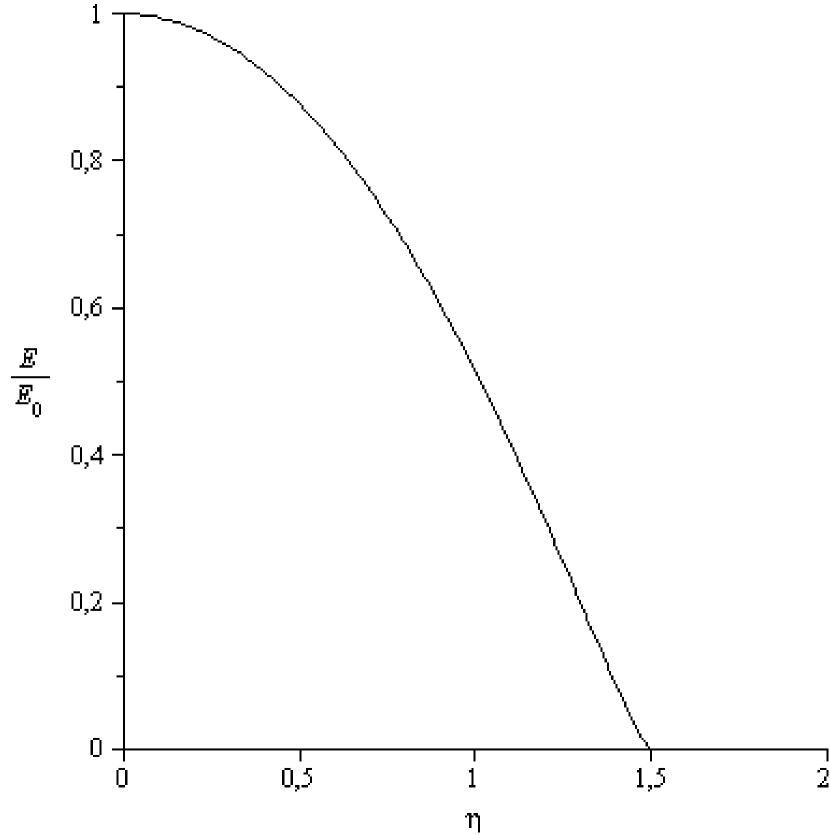
(a)

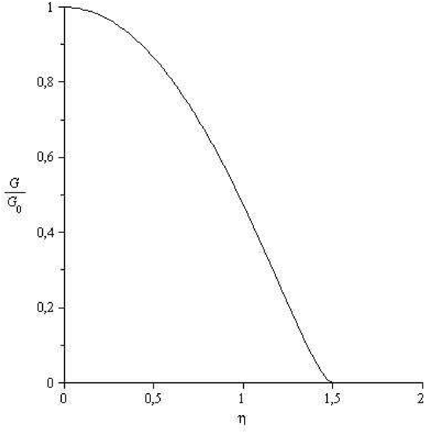
(b)

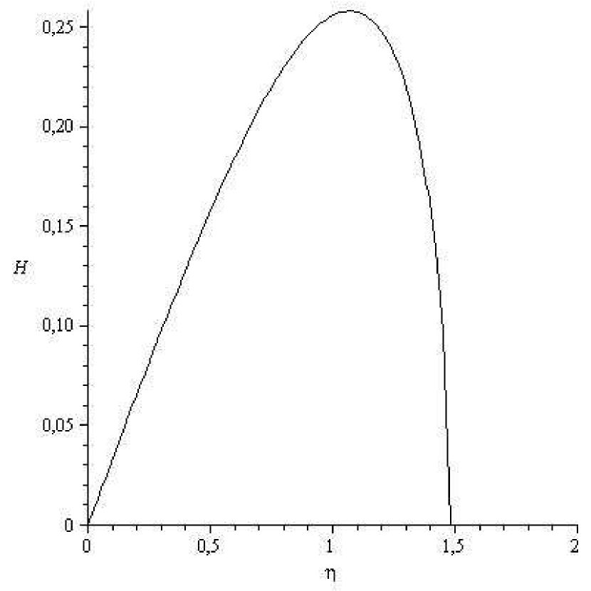
(c)

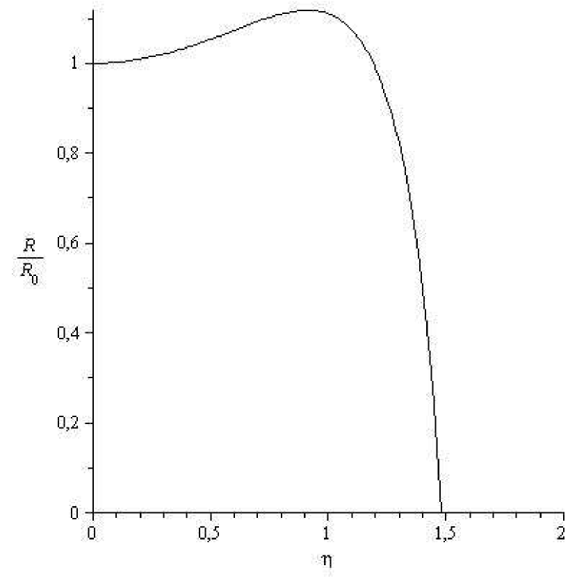
(d)

Figure 1: Calculated profiles as $\xi=0$: (a) normed profile of $E$, (b) normed profile of $G$, (c) profile of $H$, (d) normed profile of $R$.

The system of ODEs (39)–(43) satisfying boundary conditions (44), (45) was solved numerically. Additional difficulties are caused by the fact that the coefficients of ODEs have singularities. The problem was solved by the modified shooting method and asymptotic expansion of the solution in the vicinity of the singular point [3, 15]

$$E=c_{1}(\tau-a)^{10/7}+o\big{(}|\tau-a|^{10/7}\big{)},\qquad G=-\frac{30C_{e}c_{1}^{2}}{7a}(\tau-a)^{13/7}+o\big{(}|\tau-a|^{13/7}\big{)},$$

$$H=\frac{7C_{\rho}}{a(7C_{\rho}-10C_{e})}(\tau-a)+o(|\tau-a|),$$

$$R_{1}=\frac{49C_{\rho}^{2}(7(2a+1)C_{\rho}-20aC_{e})}{2a^{2}(7C_{\rho}-10C_{e})^{2}(5C_{e}-7{C_{\rho}}_{1})}(\tau-a)^{2}+o\big{(}|\tau-a|^{2}\big{)},$$

$$R_{2}=\frac{7C_{\rho}}{2(5C_{e}-7{C_{1}}_{\rho})}(\tau-a)^{2}+o\big{(}|\tau-a|^{2}\big{)}.$$

The value of $\alpha$ is taken to be $0.23$ in accordance with experimental data [9, 17]. The results for the problem solution are illustrated in Figs. 1 and 2. Fig. 1 shows the profiles of the functions $E/E_{0}$, $G/G_{0}$, $H$, and $R/R_{0}$ as $\xi=0$, where subscript $0$ denotes the axial value. The functions $E/E_{0}$, $G/G_{0}$, $H$, and $R/R_{0}$ are plotted in Fig. 2. The functions $E/E_{0}$ and $G/G_{0}$ are bell-shaped and determine shapes of the normalized turbulent kinetic energy and the normalized kinetic energy dissipation rate respectively. Similarly, $H$ and $R/R_{0}$ determine shapes of the average density defect and the normalized density fluctuation varience respectively.

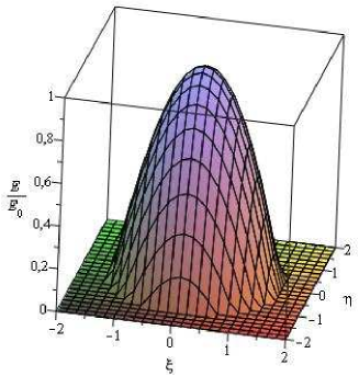
(a)

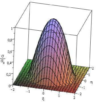
(b)

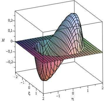
(c)

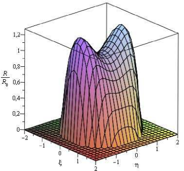
(d)

Figure 2: Calculated functions: (a) the function $E/E_{0}$, (b) the function $G/G_{0}$, (c) the function $H$, (d) the function $R/R_{0}$.

The function $H(0,\eta)$ characterizing the degree of fluid mixing in the turbulent wake is given in Fig. 1c. The maximum value of this function equals $0.258$. This is in consistent with the present notions of incomplete fluid mixing in the wakes [23, 24].

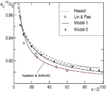
Figure 3: Axial values of the turbulent energy.

In Fig. 3 adapted from [6] the normalized values of the turbulent energy along the wake axis $e_{0}^{1/2}/U_{0}=e(x,0,0)/U_{0}$ are compared with experimental data [17], computational results [9] and results of numerical simulation based on two semi-empirical turbulence models (Model1 and Model2 in [4, 6]). The coordinate $x$ is normalized by the body diameter $D$. The results obtained here are in close agreement with Lin and Pao’s experimental data.

Acknowledgements

The authors are grateful to Professor G.G. Chernykh for many helpful and stimulating discussions. The authors would like to thank unknown referees for valuable comments which corrected and improved the first version of this paper. This work was supported by the Russian Foundation for Basic Research (project no. 10-01-00435) and programme ‘Leading scientific schools’ (grant no. NSh-544.2012.1).

References

[1]
Andreev V.K., Kaptsov O.V., Pukhnachov V.V., Rodionov A.A., Applications of
group theoretical methods in hydrodynamics, Mathematics and its
Applications, Vol. 450, Kluwer Academic Publishers, Dordrecht, 1998.
[2]
Barenblatt G.I., Galerkina N.L., Luneva M.V., Evolution of a turbulent burst,
J. Eng. Phys. Thermophys.53 (1987), 1246–1252.
[3]
Cazalbou J.B., Spalart P.R., Bradshaw P., On the behavior of two-equation
models at the edge of a turbulent region, Phys. Fluids6
(1994), 1797–1804.
[4]
Chashechkin Yu.D., Chernykh G.G., Voropaeva O.F., The propagation of a passive
admixture from a local instantaneous source in a turbulent mixing zone,
Int. J. Comp. Fluid Dyn.19 (2005), 517–529.
[5]
Chernykh G.G., Fedorova N.N., Moshkin N.P., Numerical simulation of turbulent
wakes, Russian J. Theor. Appl. Mech.2 (1992), 295–304.
[6]
Chernykh G.G., Fomina A.V., Moshkin N.P., Numerical models for turbulent wake
dynamics behind a towed body in a linearly stratified medium,
Russian J. Numer. Anal. Math. Modelling21 (2006),
395–424.
[7]
Efremov I.A., Kaptsov O.V., Chernykh G.G., Self-similar solutions of two
problems of free turbulence, Mat. Model.21 (2009),
137–144 (in Russian).
[8]
Gibson M.M., Launder B.E., On the calculation of horizontal, turbulent, free
shear flows under gravitational influence, J. Heat Transfer98 (1976), 81–87.
[9]
Hassid S., Collapse of turbulent wakes in stable stratified media,
J. Hydronautics14 (1980), 25–32.
[10]
Hinze J.O., Turbulence: an introduction to its mechanism and theory,
McGraw-Hill Series in Mechanical Engineering, McGraw-Hill Book Co., Inc., New
York, 1959.
[11]
Hulshof J., Self-similar solutions of Barenblatt’s model for turbulence,
SIAM J. Math. Anal.28 (1997), 33–48.
[12]
Kaptsov O.V., -determining equations: applications to nonlinear partial
differential equations, European J. Appl. Math.6 (1995),
265–286.
[13]
Kaptsov O.V., Efremov I.A., Invariant properties of the far turbulent wake
model, Comput. Technol.10 (2005), no. 6, 45–51 (in
Russian).
[14]
Kaptsov O.V., Efremov I.A., Schmidt A.V., Self-similar solutions of the
second-order model of the far turbulent wake, J. Appl. Mech. Tech.
Phys.49 (2008), 217–221.
[15]
Kaptsov O.V., Shan’ko Yu.V., Family of self-similar solutions of one model of
the far turbulent wake, in Proceedinds of International Conference
“Computational and Information Technologies in Sciences, Engineering, and
Education” (September 20–22, 2006, Pavlodar, Kazakhstan), Vol. 1, TOO NPF
“EKO”, Pavlodar, 2004, 576–579 (in Russian).
[17]
Lin J.T., Pao Y.H., Wakes in stratified fluids, Ann. Rev. Fluid Mech.11 (1979), 317–338.
[18]
Olver P.J., Applications of Lie groups to differential equations,
Graduate Texts in Mathematics, Vol. 107, Springer-Verlag, New York,
1986.
[19]
Ovsiannikov L.V., Group analysis of differential equations, Academic Press
Inc., New York, 1982.
[20]
Pope S.B., Turbulent flows, Cambridge University Press, Cambridge, 2000.
[21]
Rodi W., Examples of calculation methods for flow and mixing in stratified
fluids, J. Geophys. Res.92 (1987), 5305–5328.
[22]
Schlichting H., Boundary layer theory, McGraw-Hill, New York, 1955.
[23]
Vasiliev O.F., Kuznetsov B.G., Lytkin Yu.M., Cherhykh G.G., Development of the
turbulized fluid region in a stratified medium, Fluid Dyn. (1974),
no. 3, 45–52 (in Russian).
[24]
Voropaeva O.F., Far momentumless turbulent wake in a passively stratified
medium, Comput. Technol.8 (2003), no. 3, 32–46 (in
Russian).
[25]
Voropaeva O.F., Chernykh G.G., On numerical simulation of the dynamics of the
turbulized fluid regions in stratified medium, Comput. Technol.1 (1992), no. 1, 93–104 (in Russian).
[26]
Voropaeva O.F., Moshkin N.P., Chernykh G.G., Internal waves generated by
turbulent wakes in a stably stratified medium, Dokl. Phys.48 (2003), 517–521.