WASP-64 b and WASP-72 b: two new transiting highly irradiated giant planets

We report the discovery by the WASP transit survey of two new highly irradiated giant planets. WASP-64 b is slightly more massive ($1.271\pm 0.068$ $M_{Jup}$) and larger ($1.271\pm 0.039$ $R_{Jup}$) than Jupiter, and is in very-short ($a=0.02648\pm 0.00024$ AU, $P=1.5732918\pm 0.0000015$ days) circular orbit around a $V$=12.3 G7-type dwarf ($1.004\pm 0.028$ $M_{\odot}$, $1.058\pm 0.025$ $R_{\odot}$, $T_{\rm eff}$= 5500 $\pm$ 150 K). Its size is typical of hot Jupiters with similar masses. WASP-72 b has also a mass a bit higher than Jupiter’s ($1.461_{-0.056}^{+0.059}$ $M_{Jup}$) and orbits very close ($0.03708\pm 0.00050$ AU, $P=2.2167421\pm 0.0000081$ days) to a bright ($V$=9.6) and moderately evolved F7-type star ($1.386\pm 0.055$ $M_{\odot}$, $1.98\pm 0.24$ $R_{\odot}$, $T_{\rm eff}$= 6250 $\pm$ 100 K). Despite its extreme irradiation ($\sim 5.5\times 10^{9}$ erg s^-1 cm^-2), WASP-72 b has a moderate size ($1.27\pm 0.20$ $R_{Jup}$) that could suggest a significant enrichment in heavy elements. Nevertheless, the errors on its physical parameters are still too high to draw any strong inference on its internal structure or its possible peculiarity.

1 Introduction

The booming study of exoplanets allow us to assess the diversity of the planetary systems of the Milky Way and to put our own solar system in perspective. Notably, ground-based transit surveys targeting relatively bright ($V<13$) stars are detecting at an increasing rate short-period giant planets amenable for a thorough characterization (orbit, structure, atmosphere), thanks to the brightness of their host star, the favorable planet-star size ratio and their high stellar irradiation (e.g. Winn 2010). With its very high detection efficiency, the WASP transit survey (Pollacco et al. 2006) is one of the most productive projects in that domain.

In this context, we report here the detection by WASP of two new giant planets, WASP-64 b and WASP-72 b, transiting relatively bright Southern stars. Section 2 presents the WASP discovery photometry, and high-precision follow-up observations obtained from La Silla ESO Observatory (Chile) by the TRAPPIST and Euler telescopes to confirm the transits and planetary nature of both objects and to determine precisely the systems parameters. In Sect. 3, we present the spectroscopic determination of the stellar properties and the derivation of the systems parameters through a combined analysis of the follow-up photometric and spectroscopic time-series. Finally, we discuss our results in Sect. 4.

2 Observations

2.1 WASP transit detection photometry

The stars 1SWASPJ064427.63-325130.4 (WASP-64; $V$=12.3, $K$=11.0) and 1SWASPJ024409.60-301008.5 (WASP-72; $V$=10.1, $K$=9.6) were observed by the Southern station of the WASP survey (Hellier et al. 2011) between 2006 Oct 11 and 2010 Mar 12 and between 2006 Aug 11 and 2007 Dec 31, respectively. The 17981 and 6500 pipeline-processed photometric measurements were detrended and searched for transits using the methods described by Collier-Cameron et al. (2006). The selection process (Collier-Cameron et al. 2007) identified WASP-72 as a high priority candidate showing periodic low-amplitude (2-3 mmag) transit-like signatures with period of 2.217 days. For WASP-64, similar transit-like signals with a period of 1.573 days were also detected, not only on the target itself but also on a brighter star at 28”, 1SWASPJ064429.53–325129.5 (TYC7091-1288-1, $V$=12.3, $K$=11.0). Fig. 1 presents for TYC7091-1288-1 and WASP-64 the WASP photometry folded on the deduced transit ephemeris. Fig. 2 does the same for WASP-72.

A search for periodic modulation was applied to the photometry of WASP-72, using for this purpose the method described in Maxted et al. (2011). No periodic signal was found down to the mmag amplitude. We did not perform such a search for TYC7091-1288-1 and WASP-64, as these two stars are blended together at the spatial resolution of the WASP instrument (see below). Still, a Lomb-Scargle periodogram analysis of their photometric time-series did not reveal any significant power excess.

2.2 Follow-up photometry

2.2.1 WASP-64

WASP-64 is at 28” West from TYC7091-1288-1, close enough to have most of its point-spread function (PSF) enclosed in the smallest of the WASP photometry extraction apertures (radius=34”, see Fig. 3). Both objects have an entry in the WASP database, because it is based on an input catalogue of star positions. Still, the WASP light curve obtained with an aperture centered on WASP-64 is of poorer quality (see Fig. 1), because the centering algorithm does not work optimally when there is a bright object off-centre in the aperture or just outside of it, while significant levels of red noise are brought by PSF variations. This explains why the transit was first detected from the photometry centered on TYC7091-1288-1. Having both stars nearly totally enclosed in the smallest apertures for both centerings prevented us to decide from the WASP photometry alone if the eclipse signal detected by WASP was originating from one or the other star, so our first follow-up action was to measure on 2011 Jan 20 a transit at a better spatial resolution with the robotic 60cm telescope TRAPPIST (TRAnsiting Planets and PlanetesImals Small Telescope; Gillon et al. 2011, Jehin et al. 2011) located at ESO La Silla Observatory in the Atacama Desert, Chile. TRAPPIST is equipped with a thermoelectrically-cooled 2K $\times$ 2K CCD having a pixel scale of 0.65” that translates into a 22’ $\times$ 22’ field of view. Differential photometry was obtained with TRAPPIST for both stars on the night of 2011 Jan 20, corresponding to a transit window as derived from WASP data. These observations were obtained with the telescope focused and through a special ‘$I+z$’ filter that has a transmittance $>$90% from 750 nm to beyond 1100 nm. The positions of the stars on the chip were maintained to within a few pixels over the course of the run, thanks to a ‘software guiding’ system deriving regularly an astrometric solution for the most recently acquired image and sending pointing corrections to the mount if needed. After a standard pre-reduction (bias, dark, flatfield correction), the stellar fluxes were extracted from the images using the IRAF/DAOPHOT aperture photometry software (Stetson, 1987). Several sets of reduction parameters were tested, and we kept the one giving the most precise photometry for the stars of similar brightness as the target. After a careful selection of a set of 22 reference stars, differential photometry was then obtained. This reduction procedure was also applied for the subsequent TRAPPIST runs.

This first TRAPPIST run resulted in a flat light curve for TYC7091-1288-1, while the light curve for WASP-64 showed a clear transit-like structure (Fig. 3), identifying thus WASP-64 as the source of the transit signal. A second (partial) transit was observed in the $I+z$ filter on 2011 Feb 22 to better constrain the shape of the eclipse (Fig. 4, second light curve from the top). As for the following WASP-64 transits, the telescope was defocused to $\sim$3” to improve the duty cycle and average the pixel-to-pixel effects. A global analysis of the two first TRAPPIST transit light curves led to an eclipse depth and shape compatible with the transit of a giant planet in front of a solar-type star. Our next action was to observe a third transit with TRAPPIST, this time in the $V$ filter to assess the chromaticity of the transit depth (Fig. 4, third light curve from the top). The analysis of the resulting light curve led to a transit depth consistent with the one measured in the $I+z$ filter, as expected for a transiting planet. We then observed an $occultation$ window in the $z^{\prime}$-band on 2011 Apr 30. We could not detect any eclipse in the resulting photometric time-series (Fig. 5), which was again consistent with the transiting planet scenario. At this stage, we began our spectroscopic follow-up of WASP-64 that confirmed the solar-type nature of WASP-64 and the planetary nature of its eclipsing companion (see Sec. 2.3).

Once the planetary nature of WASP-64 b was confirmed, we observed seven more of its transits with TRAPPIST, using then a blue-blocking filter that has a transmittance $>$90% from 500 nm to beyond 1000 nm. The goal of using this very wide red filter is to maximize the signal-to-noise ratio (S/N) while minimizing the influence of moonlight pollution, differential extinction and stellar limb-darkening on the transit light curves. The resulting light curves are shown in Fig. 4. The transit of 2011 Oct 19 was also observed in the Gunn-$r$ filter with the EulerCam CCD camera at the 1.2-m Euler Telescope at La Silla Observatory. This nitrogen-cooled camera has a 4k $\times$ 4k E2V CCD with a 15’ $\times$ 15’ field of view (scale=0.23”/pixel). Here too, a defocus was applied to the telescope to optimize the observation efficiency and minimize pixel-to-pixel effects, while flat-field effects were further reduced by keeping the stars on the same pixels, thanks to a ‘software guiding’ system similar to the one of TRAPPIST (Lendl et al. 2012). The reduction was similar to that performed on TRAPPIST data. The resulting light curve is also shown in Fig. 4.

2.2.2 WASP-72

We monitored for WASP-72 five transits with TRAPPIST (see Table 1 and Fig. 6), two partial and two full transits in the $I+z$ filter and one full transit in the blue-blocking filter. For the three transits observed in 2011, the telescope was defocused to $\sim$3”. A first partial transit was observed in 2011 Jan 21 in the $I+z$ filter at high airmass, confirming the low-amplitude eclipse detected by WASP (Fig. 6, first light curve from the top). The next season, a full transit was observed on 2011 Oct 25 in the blue-blocking filter. A technical problem damaged these data: a shutter problem led to a scatter twice higher than expected. In 2011, a partial transit was also observed in the $I+z$ filter on Dec 4. In 2012, two new full transits were observed with TRAPPIST in the $I+z$ filter. For these two last runs, the telescope was kept focused to minimize the effects of a focus drift problem with an amplitude stronger for out-of-focus observations. We are still investigating the origin of this technical problem. Two transits of WASP-72 were also observed with Euler on 2011 Nov 26 and 2012 Nov 16, with the same strategy than for WASP-64. For the second Euler transit, a crash of the tracking system led to significant shifts of the stars on the detectors (up to 50 pixels), giving rise to significant systematic effects in the differential photometry (see Fig. 6)

Table 1 presents a summary of the follow-up photometric time-series obtained for WASP-64 and WASP-72.

Figure 1: WASP photometry for TYC7091-1288-1 ($top$) and WASP-64 ($bottom$) folded on the best-fitting transit ephemeris from the transit search algorithm presented in Collier Cameron et al. (2006), and binned per 0.01d intervals.

Figure 2: WASP photometry for WASP-72 folded on the best-fitting transit ephemeris from the transit search algorithm presented in Collier Cameron et al. (2006), and binned per 0.01d intervals.

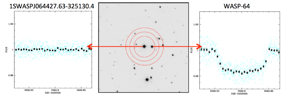
Figure 3: 280”$\times$280” TRAPPIST $I+z$ image centered on TYC7091-1288-1. North is up and East is left. The three concentric circles indicate the three photometry extraction apertures used in the WASP pipeline. WASP-64 is the closest star to the right of TYC7091-1288-1. For both stars, the light curve obtained by TRAPPIST on 2011 Jan 20 is shown (cyan=unbinned, black=binned per intervals of 0.005d).

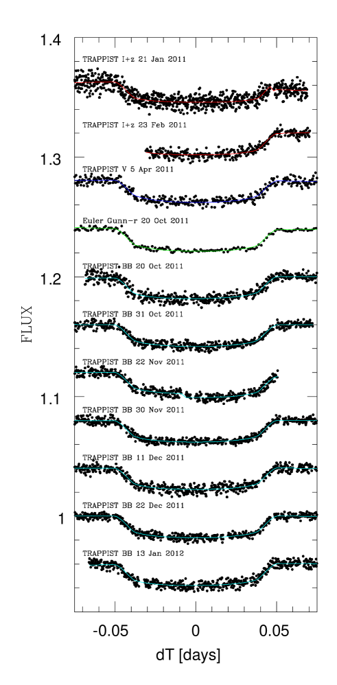
Figure 4: Follow-up transit photometry for WASP-64 b. For each light curve, the best-fit transit+baseline model deduced from the global analysis is superimposed (see Sec. 3.2). The light curves are shifted along the $y$-axis for clarity. BB = Blue-blocking filter.

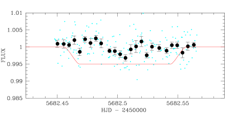
Figure 5: TRAPPIST $z^{\prime}$ time-series photometry obtained during an occultation window of WASP-64 b, unbinned and binned per intervals of 0.005d. An occultation model assuming a circular orbit and a depth of 0.5% is superimposed for comparison.

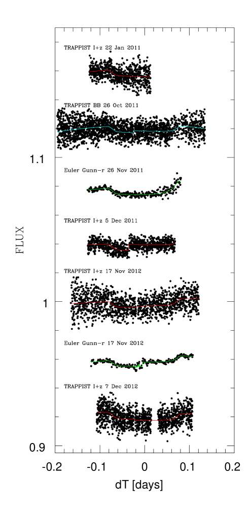
Figure 6: Follow-up transit photometry for WASP-72 b. For each light curve, the best-fit transit+baseline model deduced from the global analysis is superimposed (see Sec. 3.2). The light curves are shifted along the $y$-axis for clarity.

Target	Night	Telescope	Filter	$N$	$T_{exp}$	Baseline function	Eclipse
					(s)		nature
WASP-64	2011 Jan 20-21	TRAPPIST	$I+z$	792	8	$p(t^{2})+o$	transit
WASP-64	2011 Feb 22-23	TRAPPIST	$I+z$	296	20	$p(t^{2})$	transit
WASP-64	2011 Apr 4-5	TRAPPIST	$V$	364	30	$p(t^{2})$	transit
WASP-64	2011 Apr 30 - May 1	TRAPPIST	$z^{\prime}$	202	40	$p(t^{2})$	occultation
WASP-64	2011 Oct 19-20	TRAPPIST	BB	578	15	$p(t^{2})$	transit
WASP-64	2011 Oct 19-20	Euler	Gunn-$r$	159	60	$p(t^{2})$	transit
WASP-64	2011 Oct 30-31	TRAPPIST	BB	533	15	$p(t^{2})$	transit
WASP-64	2011 Nov 21-22	TRAPPIST	BB	512	15	$p(t^{2})+o$	transit
WASP-64	2011 Nov 29-30	TRAPPIST	BB	611	15	$p(t^{2})$	transit
WASP-64	2011 Dec 10-11	TRAPPIST	BB	642	15	$p(t^{2})+o$	transit
WASP-64	2011 Dec 21-22	TRAPPIST	BB	566	15	$p(t^{2})+o$	transit
WASP-64	2012 Jan 12-13	TRAPPIST	BB	578	15	$p(t^{2})$	transit
WASP-72	2011 Jan 21-22	TRAPPIST	$I+z$	707	8	$p(t^{2})$	transit
WASP-72	2011 Oct 25-26	TRAPPIST	BB	2042	4	$p(t^{2})+o$	transit
WASP-72	2011 Nov 25-26	Euler	Gunn-$r$	294	40	$p(t^{2})+p(a^{2})$	transit
WASP-72	2011 Dec 4-5	TRAPPIST	$I+z$	892	10	$p(t^{2})+o$	transit
WASP-72	2012 Nov 16-17	TRAPPIST	$I+z$	1344	6	$p(t^{2})+o$	transit
WASP-72	2012 Nov 16-17	Euler	Gunn-$r$	217	70	$p(t^{2}+xy^{1})+o$	transit
WASP-72	2012 Dec 6-7	TRAPPIST	$I+z$	1197	6	$p(t^{2})+o$	transit

Table 1: Summary of follow-up photometry obtained for WASP-64 and WASP-72. $N$= number of measurements. $T_{exp}$ = exposure time. BB = blue-blocking filter. The baseline functions are the analytical functions used to model the photometric baseline of each light curve (see Sec. 3.2). $p(t^{2})$ denotes a quadratic time polynomial, $p(a^{2})$ a quadratic airmass polynomial, $p(xy^{1})$ a linear function of the stellar position on the detector, and $o$ an offset fixed at the time of the meridian flip.

2.3 Spectroscopy and radial velocities

Once WASP-64 and WASP-72 were identified as high priority candidates, we gathered spectroscopic measurements with the CORALIE spectrograph mounted on Euler to confirm the planetary nature of the eclipsing bodies and obtain mass measurements. 16 usable spectra were obtained for WASP-64 from 2011 May 2 to 2011 November 7 with an exposure time of 30 minutes. For WASP-72, 18 spectra were gathered from 2011 January 9 to 2011 December 29, here too with an exposure time of 30 minutes. For both stars, radial velocities (RVs) were computed by weighted cross-correlation (Baranne et al. 1996) with a numerical G2-spectral template giving close to optimal precisions for late-F to early-K dwarfs, from our experience. The resulting RVs are shown in Table 2.

The RV time-series show variations that are consistent with planetary-mass companions. Preliminary orbital analyses of the RVs resulted in periods and phases in excellent agreement with those deduced from the WASP transit detections (Fig. 7 & 8, upper panels). For WASP-64, assuming a stellar mass $M_{\ast}=0.98\pm 0.09$ $M_{\sun}$ (Sect. 3.1), the fitted semi-amplitude $K=212\pm 17$ m s^-1 translates into a secondary mass slightly higher than Jupiter’s, $M_{p}=1.19\pm 0.12$ $M_{\rm Jup}$. The resulting orbital eccentricity is consistent with zero, $e=0.05_{-0.03}^{+0.06}$. For WASP-72, assuming a stellar mass $M_{\ast}=1.23\pm 0.10$ $M_{\sun}$ (Sect. 3.1), the fitted semi-amplitude $K=179\pm 6$ m s^-1 translates into a secondary mass $M_{p}=1.31\pm 0.08$ $M_{\rm Jup}$, while the deduced orbital eccentricity is also consistent with zero, $e=0.05_{-0.03}^{+0.03}$.

A model with a slope is slightly favored in the case of WASP-72, its value being -82 $\pm$ 22 m s^-1  per year. Indeed, the respective values for the Bayesian Information Criterion (BIC; Schwarz 1978) led to likelihood ratios (Bayes factors) between 10 and 55 in favor of the slope model, depending if the orbit was assumed to be circular or not. Such values for the Bayes factor are not high enough to be decisive, and more RVs will be needed to confirm this possible trend.

To confirm that the RV signal originates well from planet-mass objects orbiting the stars, we analyzed the CORALIE cross-correlation functions (CCF) using the line-bisector technique described in Queloz et al (2001). The bisector spans revealed to be stable, their standard deviation being close to their average error (57 $vs$ 47 m s^-1 for WASP-64 and 28 $vs$ 24 m s^-1 for WASP-72). No evidence for a correlation between the RVs and the bisector spans was found (Fig. 7 & 8, lower panels), the slopes deduced from linear regression being $-0.02\pm 0.08$ (WASP-64) and $-0.01\pm 0.04$ (WASP-72). These values and errors makes any blend scenario very unlikely. Indeed, if the orbital signal of a putative blended eclipsing binary (EB) is able to create a clear periodic wobble of the sum of both CCFs, it should also create a significant periodic distortion of its shape, resulting in correlated variations of RVs and bisector spans having the same order of magnitude (Torres et al. 2004). The power of this effect to identify blended EBs among transit candidates was first demonstrated by the classical case of CSC 01944-02289 (Mandushev et al. 2005), for which the bisector spans varied in phase with the RVs and with an amplitude about twice lower. Another famous case is the HD 41004 system (Santos et al. 2002), with a K-dwarf blended with a M-dwarf companion (separation $\sim$0.5”) which is itself orbited by a short-period brown dwarf. For this extreme system, the RVs show a clear signal at the period of the brown dwarf orbit (1.3 days) and with an amplitude $\sim 50$ m s^-1 that could be taken for the signal of a sub-Saturn mass planet orbiting the K-dwarf, except that the slope of the bisector-RV relation is $0.67\pm 0.03$, clearly revealing that the main spectral component of the CCF is not responsible for the observed signal. In the case of WASP-64 and 72, the 3-$\sigma$ upper limits of 0.23 and 0.09 that we derived from Monte-Carlo simulations for the bisector-RV slopes combined with the much higher amplitude of the measured RV signals allow us to confidently infer that the RV signal is actually originating from the target stars. This conclusion is strengthened by the consistency of the solutions derived from the global analysis of our spectroscopic and photometric data (see next Section). We conclude thus that the stars WASP-64 and WASP-72 are transited by a giant planet every $\sim$1.573 and $\sim$2.217 days, respectively. Of course, we cannot exclude that the light of those stars is not diluted by a well-aligned object able to bias our inferences about the planets. Still, our multicolor transit photometry showing no dependance of the transit depths on the wavelength, and the absence of any detectable second spectra in the CORALIE data strongly disfavors any significant pollution of the light of the host stars.

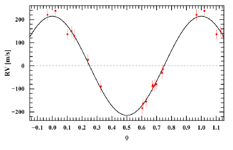
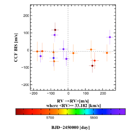
Figure 7: $Top$: CORALIE RVs for WASP-64 phase-folded on the best-fit orbital period, and with the best-fit Keplerian model over-imposed. $Bottom$: correlation diagram CCF bisector spans $vs$ RV. The colors indicate the measurement timings.

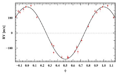
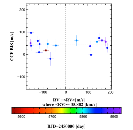
Figure 8: $Top$: CORALIE RVs for WASP-72 phase-folded on the best-fit orbital period, and with the best-fit Keplerian model over-imposed. $Bottom$: correlation diagram CCF bisector spans $vs$ RV. The colors indicate the measurement timings.

Target	$HJD_{TDB}$-2450000	RV	$\sigma_{RV}$	BS
		(km s-1)	(m s-1)	(km s-1)
WASP-64	5622.652685	33.1075	21.5	0.1171
WASP-64	5629.582507	33.3234	19.8	–0.0900
WASP-64	5681.541466	33.3368	23.9	–0.0601
WASP-64	5696.488635	33.0326	24.3	–0.0057
WASP-64	5706.460152	33.4079	24.3	–0.0156
WASP-64	5707.460947	33.0038	28.0	–0.0075
WASP-64	5708.461813	33.2129	25.1	–0.0169
WASP-64	5711.463695	33.3160	26.3	0.0040
WASP-64	5715.458133	33.1019	27.2	–0.0645
WASP-64	5716.463634	33.0977	26.1	–0.0121
WASP-64	5842.867334	33.0986	24.0	–0.0453
WASP-64	5861.847564	33.1559	25.4	0.0061
WASP-64	5864.795499	33.0230	18.1	–0.0346
WASP-64	5869.724123	33.1725	20.6	–0.0504
WASP-64	5871.734734	33.4248	21.1	0.0752
WASP-64	5872.762875	33.1044	20.1	0.0877
WASP-72	5570.618144	35.7945	13.3	0.0176
WASP-72	5828.890931	36.0233	11.3	0.0566
WASP-72	5829.865219	35.8029	9.8	0.0466
WASP-72	5830.866138	35.9320	11.5	0.0623
WASP-72	5832.894502	35.8391	14.6	0.0396
WASP-72	5852.780149	35.7640	15.5	0.0092
WASP-72	5856.757447	35.7288	11.5	0.0390
WASP-72	5858.689011	35.8146	15.2	–0.0198
WASP-72	5863.800340	35.7664	10.4	0.0462
WASP-72	5864.750293	36.0695	10.0	0.0292
WASP-72	5865.812141	35.7283	11.9	0.0968
WASP-72	5866.605265	36.0331	10.6	0.0734
WASP-72	5867.628720	35.7586	10.3	0.0605
WASP-72	5868.759336	35.9966	10.4	–0.0019
WASP-72	5873.808914	35.9928	10.9	0.0368
WASP-72	5886.748911	36.0460	16.3	0.0624
WASP-72	5914.700813	35.7261	9.5	0.0504
WASP-72	5924.584434	36.0624	10.0	0.0562

Table 2: CORALIE radial-velocity measurements for WASP-64 and WASP-72 (BS = bisector spans).

3 Analysis

3.1 Spectroscopic analysis - stellar properties

The CORALIE spectra of WASP-64 and WASP-72 were co-added to produce single spectra with average S/N of 60 and 80, respectively. The standard pipeline reduction products were used in the analysis.

The spectral analysis was performed using the methods given by Gillon et al. (2009a). The $H_{\alpha}$ line was used to determine the effective temperature ($T_{\rm eff}$). For WASP-64, the Na i D and Mg i b lines were used as surface gravity ($\log g$) diagnostics. For WASP-72, getting an measurement of $\log g$ was more critical, as the transit photometry does not constrain strongly the stellar density (see Sec. 3.2), so we used the improved method recently described by Doyle et al. (2013) and based on the ionization balance of selected Fe i/Fe ii lines in addition to the pressure-broadened Ca i lines at 6162Å and 6439Å (Bruntt et al. 2010a), along with the Na i D lines. The parameters obtained from the analysis are listed in Table 3. The elemental abundances were determined from equivalent width measurements of several clean and unblended lines. A value for microturbulence ($\xi_{\rm t}$) was determined from Fe i lines using the method of Magain (1984). The quoted error estimates include those given by the uncertainties in $T_{\rm eff}$, $\log g$  and $\xi_{\rm t}$, as well as the scatter due to measurement and atomic data uncertainties.

The projected stellar rotation velocities ($v\sin{i_{\ast}}$ ) were determined by fitting the profiles of several unblended Fe i lines. Values for macroturbulence ($v_{\rm mac}$) of 1.8 $\pm$ 0.3 and 4.0 $\pm$ 0.3 km s^-1 were assumed for WASP-64 and WASP-72, respectively, based on the calibration by Bruntt at al. (2010b). An instrumental FWHM of 0.11 $\pm$ 0.01 Å was determined for both stars from the telluric lines around 6300Å. Best-fitting values of $v\sin{i_{\ast}}$  = 3.4 $\pm$ 0.8 km s^-1  (WASP-64) and $v\sin{i_{\ast}}$  = 6.0 $\pm$ 0.7 km s^-1  (WASP-72) were obtained.

Parameter	WASP-64	WASP-72
RA (J2000)	06 44 27.61	02 44 09.60
DEC (J2000)	-32 51 30.25	-30 10 08.5
$V$	12.29	10.88
$K$	10.98	9.62
$T_{\rm eff}$	5550 $\pm$ 150 K	6250 $\pm$ 100 K
$\log g$	4.4 $\pm$ 0.15	$4.08\pm 0.13$
$\xi_{\rm t}$	0.9 $\pm$ 0.1 km s-1	1.6 $\pm$ 0.1 km s-1
$v\sin{i_{\ast}}$	3.4 $\pm$ 0.8 km s-1	6.0 $\pm$ 0.7 km s-1
[Fe/H]	$-$0.08 $\pm$ 0.11	$-$0.06 $\pm$ 0.09
[Na/H]	0.14 $\pm$ 0.08	$-$0.03 $\pm$ 0.04
[Mg/H]	0.12 $\pm$ 0.12
[Al/H]	0.00 $\pm$ 0.08
[Si/H]	0.10 $\pm$ 0.10	0.02 $\pm$ 0.07
[Ca/H]	0.05 $\pm$ 0.16	0.07 $\pm$ 0.14
[Sc/H]	0.07 $\pm$ 0.10	0.14 $\pm$ 0.07
[Ti/H]	$-$0.02 $\pm$ 0.11	0.07 $\pm$ 0.11
[V/H]	0.03 $\pm$ 0.16	$-$0.01 $\pm$ 0.08
[Cr/H]	0.01 $\pm$ 0.08	0.02 $\pm$ 0.10
[Mn/H]	0.09 $\pm$ 0.10	$-$0.11 $\pm$ 0.06
[Co/H]	0.06 $\pm$ 0.09	$-$0.06 $\pm$ 0.18
[Ni/H]	$-$0.04 $\pm$ 0.11	$-$0.04 $\pm$ 0.06
log A(Li)	$<$ 0.61 $\pm$ 0.15	$<$1.21 $\pm$ 0.17
Mass	0.98 $\pm$ 0.09 $M_{\sun}$	$1.31\pm 0.11M_{\sun}$
Radius	1.03 $\pm$ 0.20 $R_{\sun}$	$1.72\pm 0.31R_{\sun}$
Sp. Type	G7	F7
Distance	350 $\pm$ 90 pc	$340\pm 60$ pc

Table 3: Basic and spectroscopic parameters of WASP-64 and WASP-72 from spectroscopic analysis.
Notes: The values for the stellar mass, radius and surface gravity are given here for information purpose only. The values that we finally adopted for these parameters are the ones derived from the global analysis of our data (Sec. 3.2) and are presented in Table 5 and 6. Mass and radius estimate using the calibration of Torres et al. (2010). Spectral type estimated from $T_{\rm eff}$ using the table in Gray (2008).

There is no significant detection of lithium in the spectra, with equivalent width upper limits of 2mÅ for both stars, corresponding to abundance upper limits of log A(Li) $<$ 0.61 $\pm$ 0.15 (WASP-64) and log A(Li) $<$ 1.21 $\pm$ 0.17 (WASP-72). These imply ages of at least a few Gyr (Sestito & Randich, 2005).

The rotation rate for WASP-64 ($P_{\rm rot}=15.3\pm 4.7$ d) and WASP-72 ($P_{\rm rot}=14.5\pm 3.1$ d) implied by the $v\sin{i_{\ast}}$ give gyrochronological ages of $\sim$$1.2_{-0.7}^{+1.2}$ Gyr (WASP-64) and $\sim 3.7_{-1.9}^{+4.0}$ Gyr (WASP-72) under the Barnes (2007) relation.

We obtained with CORALIE two spectra of TYC7091-1288-1, the brighter star lying at 28” East from WASP-64 (Sec. 2.2.1, Fig. 3). The co-added spectrum has a S/N of only $\sim$30. A spectral analysis led to $T_{\rm eff}$$\sim$5700K and $\log g$ $\sim$4.5, with no sign of any significant lithium absorption, and a low $v\sin{i_{\ast}}$ $\sim$4 km s^-1 . The RV is $\sim$35 km s^-1 , compared to 33.2 km s^-1 for WASP-64. The cross-correlation function reveals that TYC 7091-1288-1 is an SB2 system (Fig. 8). The PPMXL catalogue (Roeser et al. 2010) shows that proper motions of both stars are consistent to within their quoted uncertainties. If these stars are physically associate, as suggested by their similar proper motions and radial velocities, their angular separation corresponds to a projected distance of 9800 $\pm$ 2500 AU, which is possible for a very wide triple system. Of course, the spectra of TYC7091-1288-1 and WASP-64 are totally separated at the spatial resolution of CORALIE (typical seeing $\sim$1”, fiber diameter of 2”), considering the 28” separation between both objects.

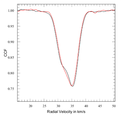
Figure 9: The cross-correlation functions for the two CORALIE spectra of TYC7091-1288-1. Their clear asymmetry indicates the SB2 nature of the star.

3.2 Global analysis

For both systems, we performed a global analysis of the follow-up photometry and the CORALIE RV measurements. The analysis was performed using the adaptive Markov Chain Monte-Carlo (MCMC) algorithm described by Gillon et al. (2012, and references therein). To summarize, we simultaneously fitted the data, using for the photometry the transit model of Mandel & Agol (2002) multiplied by a baseline model consisting of a different second-order polynomial in time for each of the light curves. We motivate the choice of this ‘minimal’ baseline model by its better ability to represent properly any smooth variation due to a combination of differential extinction and low-frequency stellar variability, compared to other possible simple functions (scalar, linear function of time or airmass). We outline that using a simple scalar as baseline model relies on the strong assumptions that the ensemble of comparison stars used to derive the differential photometry has exactly the same color than the target, that the target is perfectly stable, and that no low-frequency noise could have modified the transit shape. For eight TRAPPIST light curves (see Table 1), a normalization offset was also part of the model to represent the effect of the meridian flip. TRAPPIST’s mount is a german equatorial type, which means that the telescope has to undergo a 180^∘ rotation when the meridian is reached, resulting in different locations of the stellar images on the detector before and after the flip, and thus in a possible jump of the differential flux at the time of the flip. For the first WASP-72 Euler transit, a quadratic function of airmass had to be added to the minimal baseline model to account for the strong extinction effect caused by the high airmass ($>$2.5) at the end of the run. For the second WASP-72 transit observed by Euler, a normalization offset and a linear term in $x$- and $y$-position were added to model the effects on the photometry of the telescope tracking problem. On their side, the RVs were represented by a classical model assuming Keplerian orbits (e.g. Murray & Correia 2010, eq. 65), plus a linear trend for WASP-72 (see Sec. 2.3).

The jump parameters in our MCMC analysis were: the planet/star area ratio $(R_{p}/R_{\ast})^{2}$, the transit width (from first to last contact) $W$, the parameter $b^{\prime}=a\cos{i_{p}}/R_{\ast}$ (which is the transit impact parameter in case of a circular orbit) where $a$ is the planet’s semi-major axis and $i_{p}$ its orbital inclination, the orbital period $P$ and time of minimum light $T_{0}$, the parameter $K_{2}=K\sqrt{1-e^{2}}\textrm{ }P^{1/3}$, where $K$ is the RV orbital semi-amplitude, and the two parameters $\sqrt{e}\cos{\omega}$ and $\sqrt{e}\sin{\omega}$, where $e$ is the orbital eccentricity and $\omega$ is the argument of periastron. The choice of these two latter parameters is motivated by our will to avoid biasing the derived posterior distribution of $e$, as their use corresponds to a uniform prior for $e$ (Anderson et al. 2011).

We assumed a uniform prior distribution for all these jump parameters. The photometric baseline model parameters and the systemic radial velocity of the star $\gamma$ (and the slope of the trend for WASP-72) were not actual jump parameters; they were determined by least-square minimization at each step of the MCMC.

We assumed a quadratic limb-darkening law, and we allowed the quadratic coefficients $u_{1}$ and $u_{2}$ to float in our MCMC analysis, using as jump parameters not these coefficients themselves but the combinations $c_{1}=2\times u_{1}+u_{2}$ and $c_{2}=u_{1}-2\times u_{2}$ to minimize the correlation of the uncertainties (Holman et al. 2006). To obtain a limb-darkening solution consistent with theory, we used normal prior distributions for $u_{1}$ and $u_{2}$ based on theoretical values and 1-$\sigma$ errors interpolated in the tables by Claret (2000; 2004) and shown in Table 4. For our two non-standard filters ($I+z$ and blue-blocking), we estimated the effective wavelength basing on the transmission curves of the filters, the quantum efficiency curve of the camera and the spectral energy distributions of the stars (assumed to emit as blackbodies), and we interpolated the corresponding limb-darkening coefficient values in Claret’s tables and estimated their errors by using the values for the two nearest standard filters. We tested the insensitivity of our results to the details of this interpolation by performing short MCMC analyses with different prior distributions for the limb-darkening coefficients of the non-standard filters (e.g. assuming $I+z$ = $I$-Cousins, blue-blocking = $R$-Cousins, etc.) which led to results fully consistent with those of our nominal analysis. Such tests had also been performed in the past for other WASP planets, with similar results (e.g. Smith et al. 2012).

Limb-darkening coefficient	WASP-64	WASP-72
$u1_{V}$	$0.50\pm 0.035$	-
$u2_{V}$	$0.23\pm 0.025$	-
$u1_{Gunn-r}$	$0.43\pm 0.03$	$0.31\pm 0.015$
$u2_{Gunn-r}$	$0.26\pm 0.02$	$0.315\pm 0.005$
$u1_{BB}$	$0.36\pm 0.05$	$0.255\pm 0.04$
$u2_{BB}$	$0.255\pm 0.02$	$0.305\pm 0.01$
$u1_{I+z}$	$0.29\pm 0.03$	$0.205\pm 0.02$
$u2_{I+z}$	$0.255\pm 0.015$	$0.295\pm 0.01$

Table 4: Expectation and standard deviation of the normal distributions used as prior distributions for the quadratic limb-darkening coefficients $u1$ and $u2$ in our MCMC analysis.

Our analysis was composed of five Markov chains of $10^{5}$ steps, the first 20% of each chain being considered as its burn-in phase and discarded. For each run the convergence of the five Markov chains was checked using the statistical test presented by Gelman and Rubin (1992). The correlated noise present in the light curves was taken into account as described by Gillon et al. (2009b), by comparing the scatters of the residuals in the original and in time-binned versions of the data, and by rescaling the errors accordingly. For the WASP-72 RVs, a ‘jitter’ noise of 5.1 m s^-1   was added quadratically to the error bars, to equalize the mean error with the $rms$ of the best-fitting model residuals.

At each step of the Markov chains the dynamical stellar density $\rho_{\ast}$ deduced from the jump parameters (b’, W, $(R_{p}/R_{\ast})^{2}$, $\sqrt{e}\cos{\omega}$, $\sqrt{e}\sin{\omega}$, $P$; see, e.g., Winn 2010) and values for $T_{\rm eff}$ and [Fe/H] drawn from the normal distributions deduced from our spectroscopic analysis (Sect. 3.1), were used to determine a value for the stellar mass $M_{\ast}$ through an empirical law $M_{\ast}$($\rho_{\ast}$, $T_{\rm eff}$, [Fe/H]) (Enoch et al. 2010; Gillon et al. 2011) calibrated using the parameters of the extensive list of stars belonging to detached eclipsing binary systems presented by Southworth (2011). For WASP-64, the list was restricted to the 113 stars with a mass between 0.5 and 1.5 $M_{\odot}$, while the 212 stars with a mass between 0.7 to 1.7 $M_{\odot}$ were used for WASP-72, the goal of this selection being to benefit from our preliminary estimation of the stellar mass (Sec. 3.1, Table 3) to improve the determination of the physical parameters while using a number of calibration stars large enough to avoid small number statistical effects. To propagate properly the errors on the calibration law, the parameters of the selected subset of eclipsing binary stars were normally perturbed within their observational error bars and the coefficients of the law were redetermined at each MCMC step. Using the resulting stellar mass, the physical parameters of the system were then deduced from the jump parameters. In this procedure to derive the physical parameters of the system, the spectroscopic stellar gravity is thus not used, the stellar density deduced from the dynamical + transit parameters constraining by itself the evolutionary state of the star (Sozzetti et al. 2007). Still, for WASP-72 we assumed a normal prior distribution for $\log g$ based on the spectroscopic value and error bar (Table 3), because the low transit depth combined with the significant level of correlated noise of our data led to relatively poor constraint on the stellar density from the photometry alone (error of 50%).

For both systems, two analyses were performed, one assuming a circular orbit and the other an eccentric orbit. For the sake of completeness, the derived parameters for both models are shown in Table 5 (WASP-64) and Table 6 (WASP-72), while the best-fit transit models are shown in Fig. 10 and 11 for the circular model. Using the BIC as proxy for the model marginal likelihood, the resulting Bayes factors are $\sim$3000 (WASP-64) and $\sim$5000 (WASP-72) in favor of the circular models. A circular orbit is thus favored for both systems, and we adopt the corresponding results as our nominal solutions (right columns of Table 5 and 6). This choice is strengthened by the modeling of the tidal evolution of both planets, as discussed in Sec. 4.

3.2.1 Stellar evolution modeling

After the completion of the MCMC analyses described above, we performed for both systems a stellar evolution modeling based on the code CLES (Scuflaire et al. 2008) and on the Levenberg-Marquardt optimization algorithm (Press et al. 1992), using as input the stellar densities deduced from the MCMC, and the effective temperatures and metallicities deduced from our spectroscopic analyses, with the aim to assess the reliability of the deduced physical parameters and to estimate the age of the systems. The resulting stellar masses were $0.95\pm 0.05$ $M_{\odot}$ (WASP-64) and $1.34\pm 0.11$ $M_{\odot}$ (WASP-72), consistent with the MCMC results, while the resulting ages were $7.0\pm 3.5$ (WASP-64) and $3.2\pm 0.6$ Gy (WASP-72).

Unlike WASP-64, WASP-72 appears to be significantly evolved. To check further the reliability of our inferences for the system, we derived its parameters using the solar calibrated value of the mixing length parameter and a value 20% lower, and we also investigated the effects of convective core overshooting and microscopic diffusion of helium. All the results are within 1sigma for the mean density and surface metallicity, and within 1.5 sigma for the effective temperature, however the best fits of mean density and $T_{eff}$ are found for models including convective core overshooting. Solutions with standard physics tend to produce mean density higher than 0.2 and $T_{eff}$ higher than 6300K.

3.2.2 Global analysis of the transits with free timings

As a complement to our global analysis, we performed for both systems another global analysis with the timing of each transit being free parameters in the MCMC. The goal here was to benefit from the strong constraint brought on the transit shape provided by the total data set to derive accurate transit timings and to assess the transit periodicity. In this analysis, the parameters $T_{0}$ and $P$ were kept under the control of normal prior distributions based on the values shown for a circular orbit in Table 5 (WASP-64) and Table 6 (WASP-72), and we added a timing offset as jump parameter for each transit. The orbits were assumed to be circular. The resulting transit timings and their errors are shown in Table 7. This table also shows (last column) the resulting transit timing variations (TTV = observed minus computed timing, O-C). These TTVs are shown as a function of the transit epochs in Fig. 12. They are all compatible with zero, i.e. there is no sign of transit aperiodicity.

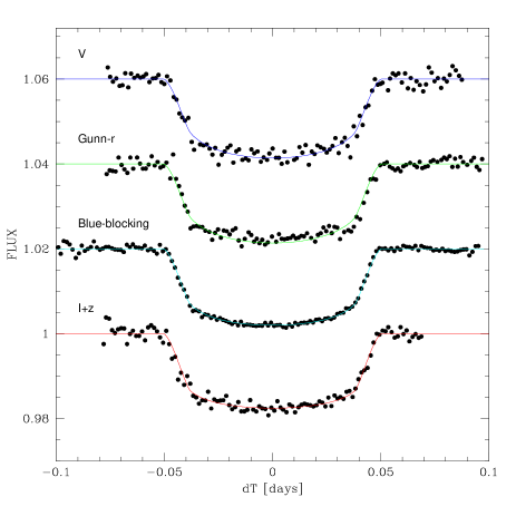
Figure 10: Combined follow-up transit photometry for WASP-64 b, detrended, period-folded and binned per intervals of 2 min. For each filter, the best-fit transit model from the global MCMC analysis is superimposed. The $V$, Gunn-$r$ and blue-blocking light curves are shifted along the $y$-axis for the sake of clarity.

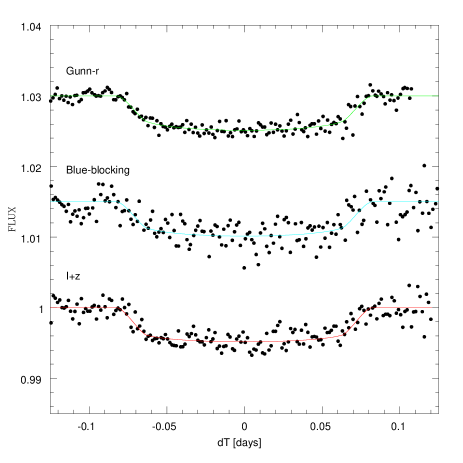
Figure 11: Combined follow-up transit photometry for WASP-72 b, detrended, period-folded and binned per intervals of 2 min. For each filter, the best-fit transit model from the global MCMC analysis is superimposed. The Gunn-$r$ and blue-blocking light curves are shifted along the $y$-axis for the sake of clarity.

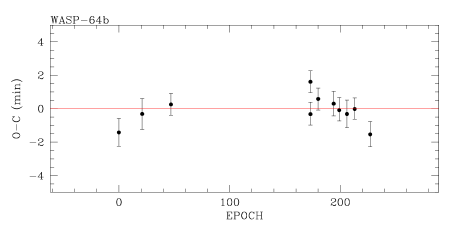
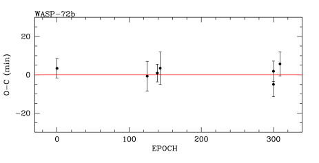
Figure 12: TTVs ($O-C$ = observed minus computed timing) derived from the global MCMC analyzes of the WASP-64 b (top) and WASP-72 b (bottom) transits (see Sec. 3.2.1).

	WASP-64
$Free$ $parameters$	$e\geq 0$	$e=0$ (adopted)
Planet/star area ratio $(R_{p}/R_{\ast})^{2}$ [%]	$1.524\pm 0.025$	$1.522\pm 0.025$
$b^{\prime}=a\cos{i_{p}}/R_{\ast}$ [$R_{*}$]	$0.321_{-0.065}^{+0.046}$	$0.322_{-0.068}^{+0.048}$
Transit width $W$ [d]	$0.10005\pm 0.00047$	$0.09999\pm 0.00046$
$T_{0}-2450000$ [$HJD_{TDB}$]	$5582.60171\pm 0.00026$	$5582.60169\pm 0.00027$
Orbital period $P$ [d]	$1.5732918\pm 0.0000015$	$1.5732918\pm 0.0000015$
RV $K_{2}$ [m s-1 d1/3]	$248\pm 14$	$257\pm 11$
RV $\gamma$ [km s-1]	$33.191\pm 0.010$	$33.1854\pm 0.0057$
$\sqrt{e}\cos{\omega}$	$0.083_{-0.088}^{+0.081}$	0 (fixed)
$\sqrt{e}\sin{\omega}$	$-0.10\pm 0.15$	0 (fixed)
$c1_{V}$	$1.167\pm 0.058$	$1.168\pm 0.058$
$c2_{V}$	$0.017\pm 0.056$	$0.016\pm 0.061$
$c1_{Gunn-r}$	$0.983\pm 0.050$	$0.985\pm 0.050$
$c2_{Gunn-r}$	$-0.121\pm 0.044$	$-0.122\pm 0.045$
$c1_{BB}$	$1.040\pm 0.045$	$1.041\pm 0.045$
$c2_{BB}$	$-0.129\pm 0.053$	$-0.125\pm 0.051$
$c1_{I+z}$	$0.859\pm 0.053$	$0.856\pm 0.053$
$c2_{I+z}$	$-0.206\pm 0.041$	$-0.208\pm 0.0241$
$T_{eff}$ [K] a	$5400\pm 100$	$5400\pm 100$
[Fe/H] a	$-$0.08 $\pm$ 0.11	$-$0.08 $\pm$ 0.11
$Deduced$ $stellar$ $parameters$
Density $\rho_{*}$ [$\rho_{\odot}$]	$0.90_{-0.09}^{+0.16}$	$0.849_{-0.044}^{+0.053}$
Surface gravity $\log g_{*}$ [cgs]	$4.406_{-0.029}^{+0.044}$	$4.392\pm 0.016$
Mass $M_{\ast}$ [$M_{\odot}$]	$0.993_{-0.037}^{+0.034}$	$1.004\pm 0.028$
Radius $R_{\ast}$ [$R_{\odot}$]	$1.036_{-0.065}^{+0.046}$	$1.058\pm 0.025$
Luminosity $L_{\ast}$ [$L_{\odot}$]	$0.90\pm 0.15$	$0.95\pm 0.13$
$u1_{V}$	$0.470\pm 0.033$	$0.470\pm 0.035$
$u2_{V}$	$0.226\pm 0.027$	$0.227\pm 0.028$
$u1_{Gunn-r}$	$0.369\pm 0.027$	$0.370\pm 0.027$
$u2_{Gunn-r}$	$0.245\pm 0.020$	$0.246\pm 0.020$
$u1_{BB}$	$0.391\pm 0.025$	$0.392\pm 0.025$
$u2_{BB}$	$0.259\pm 0.023$	$0.259\pm 0.022$
$u1_{I+z}$	$0.302\pm 0.028$	$0.301\pm 0.028$
$u2_{I+z}$	$0.255\pm 0.017$	$0.255\pm 0.018$
$Deduced$ $planet$ $parameters$
RV $K$ [m s-1 ]	$214\pm 13$	$221\pm 11$
$R_{p}/R_{\ast}$	$0.1234\pm 0.0011$	$0.1234\pm 0.0011$
$b_{tr}$ [$R_{\ast}$]	$0.313_{-0.064}^{+0.049}$	$0.322_{-0.068}^{+0.048}$
$b_{oc}$ [$R_{\ast}$]	$0.296_{-0.070}^{+0.059}$	$0.322_{-0.068}^{+0.048}$
$T_{oc}-2450000$ [$HJD_{TDB}$]	$5583.403_{-0.024}^{+0.026}$	$5583.38834\pm 0.00029$
Orbital semi-major axis $a$ [AU]	$0.02640_{-0.00033}^{+0.00030}$	$0.02648\pm 0.00024$
$a/R_{\ast}$	$5.49_{-0.19}^{+0.31}$	$5.39_{-0.09}^{+0.11}$
Orbital inclination $i_{p}$ [deg]	$86.69_{-0.66}^{+0.79}$	$86.57_{-0.60}^{+0.80}$
Orbital eccentricity $e$	$0.035_{-0.025}^{+0.039}$, $<0.132$ (95%)	0 (fixed)
Argument of periastron $\omega$ [deg]	$308_{-36}^{+80}$	-
Equilibrium temperature $T_{eq}$ [K]b	$1672_{-63}^{+59}$	$1689\pm 49$
Density $\rho_{p}$ [$\rho_{\rm Jup}$]	$0.64_{-0.08}^{+0.12}$	$0.619_{-0.052}^{+0.064}$
Surface gravity $\log g_{p}$ [cgs]	$3.294_{-0.043}^{+0.049}$	$3.292\pm 0.030$
Mass $M_{p}$ [$M_{\rm Jup}$]	$1.217\pm 0.083$	$1.271\pm 0.068$
Radius $R_{p}$ [$R_{\rm Jup}$]	$1.244_{-0.080}^{+0.062}$	$1.271\pm 0.039$

Table 5: Median and 1-$\sigma$ limits of the marginalized posterior distributions obtained for the WASP-64 system parameters as derived from our MCMC analysis. ^aUsing as priors the spectroscopic values given in Table 3. ^bAssuming a null Bond albedo ($A_{B}$=0) and isotropic reradiation ($f$=1/4).

	WASP-72
$Free$ $parameters$	$e\geq 0$	$e=0$ (adopted)
Planet/star area ratio $(R_{p}/R_{\ast})^{2}$ [%]	$0.423_{-0.037}^{+0.039}$	$0.430_{-0.039}^{+0.043}$
$b^{\prime}=a\cos{i_{p}}/R_{\ast}$ [$R_{*}$]	$0.58_{-0.20}^{+0.10}$	$0.59_{-0.18}^{+0.10}$
Transit width $W$ [d]	$0.1552\pm 0.0029$	$0.1558_{-0.0029}^{+0.0035}$
$T_{0}-2450000$ [$HJD_{TDB}$]	$5583.6525\pm 0.0021$	$5583.6529\pm 0.0021$
Orbital period $P$ [d]	$2.2167434_{-0.0000077}^{+0.0000084}$	$2.2167421\pm 0.0000081$
RV $K_{2}$ [m s-1 d1/3]	$236.6\pm 5.6$	$236.1\pm 5.5$
RV $\gamma$ [km s-1]	$35.923\pm 0.015$	$35.919\pm 0.014$
RV slope [m s-1 y-1]	$-44\pm 19$	$-39\pm 17$
$\sqrt{e}\cos{\omega}$	$-0.022\pm 0.071$	0 (fixed)
$\sqrt{e}\sin{\omega}$	$-0.06\pm 0.11$	0 (fixed)
$c1_{Gunn-r}$	$0.938\pm 0.026$	$0.936\pm 0.026$
$c2_{Gunn-r}$	$-0.318\pm 0.016$	$-0.319\pm 0.017$
$c1_{BB}$	$0.820\pm 0.082$	$0.818\pm 0.078$
$c2_{BB}$	$-0.352\pm 0.046$	$-0.352\pm 0.042$
$c1_{I+z}$	$0.713\pm 0.041$	$0.710\pm 0.042$
$c2_{I+z}$	$-0.382\pm 0.028$	$-0.383\pm 0.027$
$T_{eff}$ [K] a	$6250\pm 100$	$6250\pm 100$
[Fe/H] a	$-$0.06 $\pm$ 0.09	$-$0.06 $\pm$ 0.09
$Deduced$ $stellar$ $parameters$
Surface gravity $\log g_{*}$ [cgs] a	$3.99\pm 0.10$	$3.99_{-0.11}^{+0.10}$
Density $\rho_{*}$ [$\rho_{\odot}$]	$0.181_{-0.046}^{+0.074}$	$0.177_{-0.048}^{+0.073}$
Mass $M_{\ast}$ [$M_{\odot}$]	$1.382\pm 0.053$	$1.386\pm 0.055$
Radius $R_{\ast}$ [$R_{\odot}$]	$1.97\pm 0.23$	$1.98\pm 0.24$
Luminosity $L_{\ast}$ [$L_{\odot}$]	$5.3_{-1.2}^{+1.4}$	$5.3_{-1.3}^{+1.5}$
$u1_{Gunn-r}$	$0.311\pm 0.013$	$0.311\pm 0.013$
$u2_{Gunn-r}$	$0.3148\pm 0.0063$	$0.3147\pm 0.0060$
$u1_{BB}$	$0.257\pm 0.043$	$0.256\pm 0.041$
$u2_{BB}$	$0.305\pm 0.013$	$0.305\pm 0.014$
$u1_{I+z}$	$0.209\pm 0.022$	$0.208\pm 0.022$
$u2_{I+z}$	$0.295\pm 0.012$	$0.295\pm 0.013$
$Deduced$ $planet$ $parameters$
RV $K$ [m s-1 ]	$181.3\pm 4.2$	$181.0\pm 4.2$
$R_{p}/R_{\ast}$	$0.0650\pm 0.0029$	$0.0656\pm 0.0031$
$b_{tr}$ [$R_{\ast}$]	$0.57_{-0.20}^{+0.10}$	$0.59_{-0.18}^{+0.10}$
$b_{oc}$ [$R_{\ast}$]	$0.58_{-0.21}^{+0.11}$	$0.59_{-0.18}^{+0.10}$
$T_{oc}-2450000$ [$HJD_{TDB}$]	$5584.758\pm 0.042$	$5584.7612\pm 0.0021$
Orbital semi-major axis $a$ [AU]	$0.03705\pm 0.00047$	$0.03708\pm 0.00050$
$a/R_{\ast}$	$4.05_{-0.38}^{+0.49}$	$4.02_{-0.40}^{+0.49}$
Orbital inclination $i_{p}$ [deg]	$81.8_{-2.5}^{+3.5}$	$81.6_{-2.6}^{+3.2}$
Orbital eccentricity $e$	$0.014_{-0.010}^{+0.018}$, $<0.079$ (95%)	0 (fixed)
Argument of periastron $\omega$ [deg]	$115_{-47}^{+111}$	-
Equilibrium temperature $T_{eq}$ [K]b	$2200_{-120}^{+110}$	$2210_{-130}^{+120}$
Density $\rho_{p}$ [$\rho_{\rm Jup}$]	$0.75_{-0.25}^{+0.45}$	$0.72_{-0.25}^{+0.43}$
Surface gravity $\log g_{p}$ [cgs]	$3.37_{-0.11}^{+0.13}$	$3.36\pm 0.12$
Mass $M_{p}$ [$M_{\rm Jup}$]	$1.459\pm 0.056$	$1.5461_{-0.056}^{+0.059}$
Radius $R_{p}$ [$R_{\rm Jup}$]	$1.25\pm 0.19$	$1.27\pm 0.20$

Table 6: Median and 1-$\sigma$ limits of the marginalized posterior distributions obtained for the WASP-72 system parameters as derived from our MCMC analysis. ^aUsing as priors the spectroscopic values given in Table 3. ^bAssuming a null Bond albedo ($A_{B}$=0) and isotropic reradiation ($f$=1/4).

Planet	Epoch	Transit timing - 2450000	$O-C$
		[$HJD_{TDB}$]	[$s$]
WASP-64 b	0	$5582.60070\pm 0.00051$	$-85\pm 50$
	21	$5615.64057\pm 0.00057$	$-19\pm 55$
	47	$5656.54655\pm 0.00035$	$+15\pm 39$
	173	$5854.78224\pm 0.00027$	$+97\pm 40$
	173	$5854.78091\pm 0.00032$	$-19\pm 41$
	180	$5865.79456\pm 0.00025$	$+35\pm 39$
	194	$5887.82045\pm 0.00035$	$+18\pm 44$
	199	$5895.68667\pm 0.00029$	$-5\pm 42$
	206	$5906.69953\pm 0.00041$	$-19\pm 50$
	213	$5917.71279\pm 0.00019$	$-1\pm 38$
	229	$5939.73781\pm 0.00030$	$-92\pm 45$
WASP-72 b	0	$5583.6542\pm 0.0024$	$+3.3\pm 5.0$
	125	$5860.7441\pm 0.0048$	$-0.7\pm 7.7$
	139	$5891.7797\pm 0.0017$	$+0.9\pm 4.6$
	143	$5900.6475\pm 0.0043$	$+3.4\pm 8.5$
	300	$6248.6710\pm 0.0029$	$-5.0\pm 6.4$
	300	$6248.6758\pm 0.0012$	$+1.8\pm 5.3$
	309	$6268.6292\pm 0.0024$	$+5.7\pm 6.3$

Table 7: Transit timings and TTVs ($O-C$ = observed minus computed timing) derived from the MCMC global analyzes of the WASP-64 b and WASP-72 b transits.

4 Discussion

WASP-64 b and WASP-72 b are thus two new very short-period (1.57d and 2.22d) planets slightly more massive than Jupiter orbiting moderately bright ($V$=12.3 and 10.1) Southern stars. Their detection demonstrates nicely the high photometric potential of the WASP transit survey (Pollacco et al. 2006), as both planets show transits of very low-amplitude ($<$ 0.5%) in the WASP data. For WASP-64, the reason is not the intrinsic size contrast with the host star but the dilution of the signal by a close-by spectroscopic binary that could be dynamically bound to WASP-64 (Sec. 3.1).

Fig. 13 shows the position of both planets in mass-radius and irradiation-radius diagrams for a mass range from 1 to 2 $M_{Jup}$. WASP-64 b lies in a well-populated area of the irradiation-radius diagram. Its physical dimensions can be considered as rather standard. Its measured radius of $1.27\pm 0.04$ $R_{\rm Jup}$ agrees well with the value of $1.22\pm 0.11$ $R_{Jup}$ predicted by the equation derived by Enoch et al. (2012) from a sample of 71 transiting planets with a mass between 0.5 and 2 $M_{\rm Jup}$ and relating planets’ sizes to their equilibrium temperatures and semi-major axes. On the contrary, WASP-72 b appears to be a possible outlier, its measured radius of $1.27\pm 0.20$ $R_{\rm Jup}$ being marginally lower than the value predicted by Enoch et al’s empirical relation, $1.70\pm 0.11$ $R_{Jup}$. Its density of $0.732_{-0.25}^{+0.43}$ $\rho_{\rm Jup}$ could indeed be considered as surprisingly high given its extreme irradiation ($\sim 5.5\times 10^{9}$ erg s^-1 cm^-2), suggesting a possible enrichment of heavy elements. Nevertheless, Fig. 13 clearly shows that the errors on its physical parameters are still too high to draw any strong inference on its internal structure or its possible peculiarity. Indeed, the transit parameters are still loosely determined, especially the impact parameter, resulting in a high relative error on the stellar density that propagates to the stellar and planetary radii. Planets with similar irradiation and mass being still rare, it will thus be especially interesting to improve these parameters with new follow-up observations.

As described in Sec. 3.2, we have adopted the circular orbital models for both planets, basing on their higher marginal likelihoods. To assess the validity of this choice on a theoretical basis, we integrated the future orbital evolution of both systems through the low-eccentricity tidal model presented by Jackson et al. (2008), assuming as starting eccentricity the 95% upper limits derived in our MCMC analysis (0.132 for WASP-64 b and 0.052 for WASP-72 b) and assuming mean values of $10^{7}$ and $10^{5}$ for, respectively, the stellar and planetary tidal dissipation parameters $Q^{\prime}_{\ast}$ and $Q^{\prime}_{p}$ (Goldreich & Soter, 1966). These integrations resulted in circularization times (defined as the time needed to reach $e<0.001$) of 4 and 24 Myr for, respectively, WASP-64 b and WASP-72 b. These times are much shorter than the estimated age of the systems, strengthening our selection of the circular orbital solutions. It is worth mentioning that both systems are tidally unstable, as most of the hot Jupiter systems (Levrard et al. 2009), the times remaining for the planets to reach their Roche limits being respectively 0.9 Gy (WASP-64 b) and 0.35 Gy (WASP-72 b) under the assumed tidal dissipation parameters.

The new transiting systems reported here represent both two interesting targets for follow-up observations. Thanks to its extreme irradiation and its moderately high planet-to-star size ratio, WASP-64 b is a good target for near-infrared occultation (spectro-)photometry programs able to probe its day-side spectral energy distribution. Assuming a null albedo for the planet and blackbody spectra for both the planet and the host star, we computed occultation depths of 650-1550 ppm in $K$-band, 1500-2750 ppm at 3.6 $\mu$m and 2050-3350 ppm at 4.5 $\mu$m, the lower and upper limits corresponding, respectively, to a uniform redistribution of the stellar radiation to both planetary hemispheres and to a direct reemission of the dayside hemisphere. Precise measurement of such occultation depths is definitely within the reach of several ground-based and space-based facilities (e.g. Gillon et al. 2012). For ground-based programs, the situation is made easier by the presence of a bright ($K=9.8$) comparison star at only 28” from the target (Fig. 3). For WASP-72, atmospheric measurements are certainly more challenging considering the lower planet-to-star size ratio. Here, the first follow-up actions should certainly be to confirm and improve our measurement of the planet’s size through high-precision transit photometry, and to gather more RVs to confirm the trend marginally detected in our analysis.

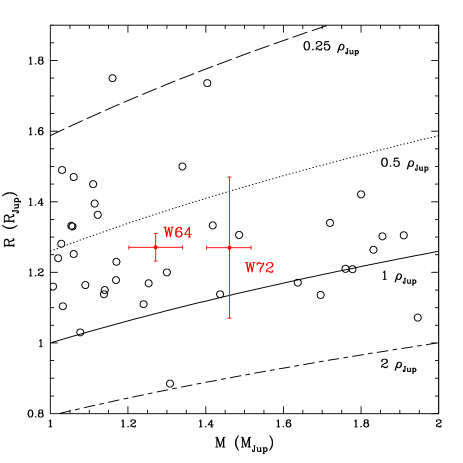
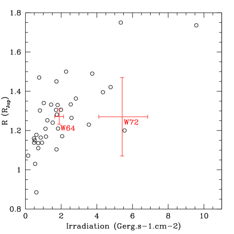
Figure 13: $Left$: mass–radius diagram for the transiting planets with masses ranging from 1 to 2 $M_{\rm Jup}$ (data from exoplanet.eu, Schneider et al. 2011). WASP-64 b and WASP-72 b are shown as red square symbols, while the other planets are shown as open circles without their error bars for the sake of clarity. Different iso-density lines are also shown. $Right$: position of WASP-64 b and WASP-72 b in a irradiation–radius diagram for the same exoplanets sample.

- (1) Anderson D. R., Collier Cameron A., Hellier C., et al. 2011, ApJL, 726, L19
- (2) Baranne A., Queloz D., Mayor M., et al., 1996, A&AS, 119, 373
- (3) Barnes, S. A. 2007, ApJ, 669, 1167
- (4) Bruntt, H., Deleuil, M., Fridlund, M., et al. 2010a, A&A, 519, A51
- (5) Bruntt, H., Bedding, T. R., Quirion, P.-O., et al. 2010b, MNRAS, 405, 1907
- (6) Claret A., 2000, A&A, 363, 1081
- (7) Claret A., 2004, A&A, 428, 1001
- (8) Collier-Cameron, A., Pollacco, D., Street, R. A., et al. 2006, MNRAS, 373, 799
- (9) Collier-Cameron, A., Wilson, D. M., West, R. G., et al. 2007, MNRAS, 380, 1230
- (10) Doyle, A. P., Smalley, B., Maxted, P. F. L., et al. 2013, MNRAS, 428, 3164
- (11) Enoch, B., Collier-Cameron, A., Parley, N. R., Hebb, L. 2010 A&A, 516, A33
- (12) Enoch, B., Collier-Cameron, A. & Horne, K. 2012, A&A, 540, A99
- (13) Gelman A., Rubin D., 1992, Statistical Science, 7, 457
- (14) Gillon, M., Smalley, B., Hebb, L., et al. 2009a, A&A, 496, 259
- (15) Gillon M., Demory B.-O., Triaud A. H. M. J., et al., 2009b, A&A, 506, 359
- (16) Gillon, M., Doyle, A. P., Lendl, M., et al. 2011, A&A, 533, A88
- (17) Gillon, M., Jehin, E., Magain, P., et al. 2011, Detection and Dynamics of Transiting Exoplanets, Proceedings of OHP Colloquium (23-27 August 2010), eds. F. Bouchy, R. F. Diaz & C. Moutou, Platypus Press, 06002
- (18) Gillon M., Triaud A. H. M. J., Fortney J. J., et al. 2012, A&A, 542, 4
- (19) Goldreich, O. & Soter, S. 1966, Icarus, 5, 375
- (20) Gray, D. F. 2008, The observation and analysis of stellar photospheres, 3rd Edition (Cambridge University Press), p. 507
- (21) Hellier, C., Anderson, D. R., Collier-Cameron, A., et al. 2011, Detection and Dynamics of Transiting Exoplanets, Proceedings of OHP Colloquium (23-27 August 2010), eds. F. Bouchy, R. F. Diaz & C. Moutou, Platypus Press, 01004
- (22) Holman M. J., Winn J. N., Latham D. W., et al., 2006, ApJ, 652, 1715
- (23) Jackson, D., Greenberg, R., & Barnes, R. 2008, ApJ, 678, 1396
- (24) Jehin, E., Gillon, M., Queloz, D., et al. 2011, The Messenger, 145, 2
- (25) Lammer, H., Odert, P., Leitzinger, M., et al. 2009, A&A, 506, 399
- (26) Lendl, M., Anderson, D. R., Collier-Cameron, A., et al. 2012, A&A, 544, A72
- (27) Levrard, B., Winisdoerffer, C. & Chabrier, G. 2009, ApJL, 692, 9
- (28) Mandel K., Agol E., 2002, ApJ, 580, 181
- (29) Mandushev, G., Torres, G., Latham, D. W., et al., 2005, ApJ, 621, 1061
- (30) Magain P., 1984, A&A, 134, 189
- (31) Maxted, P. F. L., Anderson, D. R., Collier Cameron, A., et al. 2011, PASP, 123, 547
- (32) Murray, C. D. & Correia A. C. M. 2010, Exoplanets, edited by S. Seager, University of Arizona Press, p 15-23
- (33) Pollacco, D. L., Skillen, I., Collier Cameron, A., et al. 2006, PASP, 118, 1407
- (34) Press, W. H., Teukolsly, S. A., Vetterling, W. T., Flannery B. P. 1992, Numerical recipes in FORTRAN: The art of scientific computing, 2nd Edition (Cambridge University Press)
- (35) Queloz D., Henry G. W., Sivan J. P., et al., 2001, A&A, 379, 279
- (36) Roeser, S., Demleitner, M., & Schilbach, E. 2010, AJ, 139, 2440
- (37) Santos, N., C., Mayor, M., Naef, D., et al. 2002, A&A, 392, 215
- (38) Schwarz, G. E. 1978, Annals of Statistics, 6, 461
- (39) Schneider, J., Dedieu, C., Le Sidaner, P., et al. 2011, A&A, 532, 79
- (40) Scuflaire R., Théado S., Montalbán J., et al. 2008, APSS, 316, 149
- (41) Sestito, P. & Randich, S. 2005, A&A, 442, 615
- (42) Smith, A. M. S., Anderson, D. R., Collier Cameron, A., et al. 2012, AJ, 143, 81
- (43) Southworth, J., 2011, MNRAS, 417, 2166
- (44) Sozzetti, A., Torres, G., Charbonneau, D., et al. 2007, ApJ, 664, 1190
- (45) Stetson, P. B. 1987, PASP, 99, 111
- (46) Torres, G., Konacki, M., Sasselov, D. D., Jha, S. 2005, ApJ, 619, 558
- (47) Torres, G., Andersen, J. & Giménez, A. 2010, A&A Rev., 18, 67
- (48) Winn, J. N. 2010, Exoplanets, edited by S. Seager, University of Arizona Press, p 55-77