The Second Multiple-Planet System Discovered by Microlensing: OGLE-2012-BLG-0026Lb, c,
A Pair of Jovian Planets Beyond the Snow Line

Abstract

We report the discovery of a planetary system from observation of the high-magnification microlensing event OGLE-2012-BLG-0026. The lensing light curve exhibits a complex central perturbation with multiple features. We find that the perturbation was produced by two planets located near the Einstein ring of the planet host star. We identify 4 possible solutions resulting from the well-known close/wide degeneracy. By measuring both the lens parallax and the Einstein radius, we estimate the physical parameters of the planetary system. According to the best-fit model, the two planet masses are $\sim 0.11\ M_{\rm J}$ and $0.68\ M_{\rm J}$ and they are orbiting a G-type main sequence star with a mass $\sim 0.82\ M_{\odot}$. The projected separations of the individual planets are beyond the snow line in all four solutions, being $\sim 3.8$ AU and 4.6 AU in the best-fit solution. The deprojected separations are both individually larger and possibly reversed in order. This is the second multi-planet system with both planets beyond the snow line discovered by microlensing. This is the only such a system (other than the Solar System) with measured planet masses without $\sin i$ degeneracy. The planetary system is located at a distance 4.1 kpc from the Earth toward the Galactic center. It is very likely that extra light from stars other than the lensed star comes from the lens itself. If this is correct, it will be possible to obtain detailed information about the planet-host star from follow-up observation.

1. Introduction

According to the standard theory of planet formation, rocky planets form in the inner part of the protoplanetary disk of a star, within the snow line, where the temperature is high enough to prevent the condensation of water and other substances onto grains (Raymond et al., 2007). This results in coagulation of purely rocky grains and later in the formation of rocky planets. On the other hand, formation of giant planets starts at some distance from the host star, beyond the snow line, where the low temperature of the protoplanetary disk allows for condensation of water ice, enabling more rapid accumulation of solid material into a large planetary core. The core accretes surrounding gas and later evolves into a gas giant planet (Pollack et al., 1996). Due to the difference in the conditions of formation, rocky terrestrial and gas giant planets form at different regions of planetary systems (Ida & Lin, 2004).

Planet formation theories were initially based entirely on the Solar System. Planet search surveys using the radial velocity and transit methods have discovered numerous planets, including many gas giants. Most of the giant planets have short-period orbits and are thus much closer to their parent stars than the giant planets in the Solar System. These discoveries have inspired new theoretical work, such as various migration theories to resolve the contradiction between the present-day and assumed-birth locations of giant planets. However, it is essential to discover more planets located beyond the snow line to bridge the gap between the Solar System and exo-planet systems.

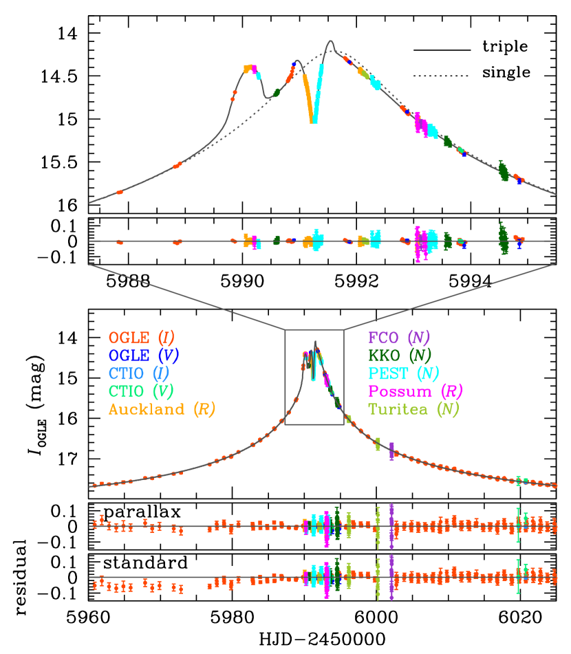
Figure 1.— Light curve of OGLE-2012-BLG-0026. The lower panel shows the whole view of the light curve and the upper panel shows an enlarged view of the perturbation. Data points taken from different observatories are marked by different colors along with the passbands of observation. The passband notation “N” represents that no filter is used. The dotted and solid curves represent the solutions from single and triple lensing modeling, respectively. The two residuals in the lower panel are presented to show the difference between the fits of the models with and without the parallax effect.

Microlensing is an important tool that can provide observational evidence to check planet formation theories. The planetary signal in a microlensing event is a short-term perturbation to the smooth standard light curve of the lensing event induced by the planet’s host star (Mao & Paczyński, 1991; Gould & Loeb, 1992). The perturbation is caused by the approach of a lensed star (source) close to the planet-induced caustics. The caustic is an optical term representing the envelope of concentrated light that forms when light ray is refracted by a curved surface, e.g. a curved region of bright light when light shines on a drinking glass filled with water or a rippling pattern at the bottom of a swimming pool. For gravitational bending of light, caustics represents the positions on the source plane at which the lensing magnification of a point source becomes infinity due to the singularity in the lens-mapping equation. When a caustic is formed by a planetary system, it forms multiple sets of closed curves each of which is composed of concave curves that meet at cusps. Among them, one set is always located close to the planet’s host star (central caustic) and other sets are located away from the star (planetary caustic). Due to these caustic locations, a perturbation induced by a central caustic (central perturbation) occurs near the peak of a high-magnification event, while a perturbation induced by a planetary caustic occurs on the wings of a lensing light curve. The caustic size, and thus the planet detection sensitivity, is maximized when the planet is located in the region near the Einstein ring of the host star, which is often referred to as the lensing zone. For a typical Galactic lensing event, the physical size of the Einstein radius is $r_{\rm E}\sim 3.0(M/M_{\odot})^{1/2}$ AU, where $M$ is the mass of the lens. This is similar to the snow line of $2.7(M/M_{\odot})^{p}$ AU, where $0.7\lesssim p\lesssim 2$ (Ida & Lin, 2005; Kennedy & Kenyon, 2008). Therefore, microlensing is an efficient method for detecting cool planets located at or beyond the snow line.

Microlensing is also sensitive to multiple-planet systems. Microlensing detection of multiple planets is possible because all planets in the lensing zone affect the magnification pattern around the primary lens (Griest & Safizadeh, 1998), and thus the signatures of the multiple planets can be detected in the light curve of a high magnification event (Gaudi et al., 1999). Indeed, the first two-planet microlensing system was discovered through this channel (Gaudi et al., 2008; Bennett et al., 2010).

In this paper, we report the second discovery of a multiple-planetary system composed of two planets located beyond the snow line discovered by using the microlensing method.

2. Observation

OGLE-2012-BLG-0026 was discovered by the Optical Gravitational Lensing Experiment Early Warning System (OGLE EWS; Udalski 2003) on 2012-Feb-13 toward the Galactic bulge at $(\alpha,\delta)_{\rm J2000}=(17^{\rm h}34^{\rm m}18^{\rm s}\hskip-2.0pt.70,-27^{\circ}08^{\prime}33^{\prime\prime}\hskip-2.0pt.9)$, i.e., $(l,b)=(0.195^{\circ},3.066^{\circ})$, based on $I$-band observations with the 1.3m Warsaw telescope at Las Companas Observatory in Chile. At HJD’ (= HJD-2450000) = 5989.3 (Mar 2), the Microlensing Follow-Up Network ($\mu$FUN) issued an alert, saying that the event would reach high magnification ($A>100$) 2.5 days hence, and urging immediate observations. Given this extremely early date (3.5 months before the target reaches opposition), and hence very short observing window from any individual site, this quick alert was crucial to mobilizing near-24-hour coverage from multiple sights. $\mu$FUN covered the peak with observations from 6 telescopes: the 0.4 m at Auckland Observatory, 0.4 m at Farm Cove Observatory (FCO), 0.4 m Possum Observatory, 0.4 m Turitea Observatory in New Zealand, 0.4 m Klein Karoo Observatory (KKO) in South Africa, and 0.3 m Perth Exoplanet Survey Telescope (PEST) in Australia. The Auckland data were taken in $R$ band, and the remainder were unfiltered. In addition, $\mu$FUN obtained supplementary $V/I/H$ color observations using the 1.3 m SMARTS telescope at Cerro Tololo Inter-American Observatory (CTIO). Follow-up observation was stopped after the perturbation, but normal monitoring of the event was continued by the OGLE survey until the event returned to its baseline brightness, and beyond.

Photometric reductions of data were carried out using photometry codes developed by the individual groups. The OGLE data were reduced by a photometry pipeline that applies the image subtraction method based on the Difference Image Analysis technique (Alard & Lupton, 1998) and further developed by Woźniak (2000) and Udalski (2003). Initial reduction of the $\mu$FUN data were processed using a pipeline based on the DoPHOT software (Schechter et al., 1993). The data were reprocessed by using the pySIS package (Albrow et al., 2009) to refine the photometry.

Figure 1 shows the light curve of OGLE-2012-BLG-0026. The magnification of the lensed source star flux reached $A_{\rm max}\sim 129$ at the peak. The perturbation is localized near the peak region of the light curve. It exhibits a complex structure with multiple features. At a glance, the perturbation is composed of two parts. One part, at ${\rm HJD}^{\prime}\sim 5990.2$ has a positive deviation with respect to the unperturbed single-lens light curve. The other part, centered at ${\rm HJD}^{\prime}\sim 5991.2$ has a negative deviation. Such a complex perturbation pattern is unusual for central perturbations.

3. Interpretation of light curve

To interpret the observed light curve, we initially conducted modeling based on a standard two-mass lens model. Description of a binary-lens light curve requires 3 single lensing parameters plus another 3 parameters related to the binary nature of the lens. The single lensing parameters include the moment of the closest lens-source approach, $t_{0}$, the projected lens-source separation at that moment, $u_{0}$, and the Einstein time scale, $t_{\rm E}$, of the event. The Einstein time scale is defined as the time required for the source to cross the angular Einstein radius of the lens, $\theta_{\rm E}$. The binary lensing parameters are the projected binary separation in units of the Einstein radius, $s$, the mass ratio between the lens components, $q$, and the angle between the source trajectory and the binary axis, $\alpha$. Since central perturbations usually involve caustic crossings or approaches, an additional parameter of the source radius in units of $\theta_{\rm E}$, $\rho_{\star}$ (normalized source radius), is needed to account for the attenuation of lensing magnifications by the finite size of the source. A central perturbation in the light curve of a high magnification event can be produced either by a planetary companion positioned in the lensing zone or by a binary companion located away from the Einstein radius (Han & Gaudi, 2008; Han, 2009). From a thorough search considering both possible cases of central perturbations, however, we could not find any solution that explains the observed perturbation.

We therefore consider the possibility of an additional lens companion. Han (2005) pointed out that many cases of central perturbations induced by multiple planets can be approximated by the superposition of the single-planet perturbations in which the individual planet-primary pairs act as independent binary lens systems. Based on this “binary superposition” approximation, we then conduct another binary lens modeling of the two light curves each of which is prepared by including only a single perturbed region. The first light curve includes the negative perturbation region during $5990.5<{\rm HJD}^{\prime}<5992.0$ and the second includes the positive perturbation region during $5989.0<{\rm HJD}^{\prime}<5990.5$. From this, we find that the two partial light curves are well fitted by binary lensing light curves with two different planetary companions.

Based on the parameters of the individual planetary companions, we then conduct triple-lens modeling, which requires to include three additional parameters related to the second companion. These are the normalized projected separation from the primary, $s_{2}$, the mass ratio between the second companion and the primary, $q_{2}$, and the position angle of the second planet with respect to the line connecting the primary and the first planet, $\psi$. We denote the parameters related to the first planet as $s_{1}$ and $q_{1}$. We note that the first and second planets are designated as the ones producing the negative and positive perturbations, respectively. With the initial values of the triple-lens parameters obtained from the binary superposition approximation, we locate the $\chi^{2}$ minimum using the Markov Chain Monte Carlo (MCMC) method.

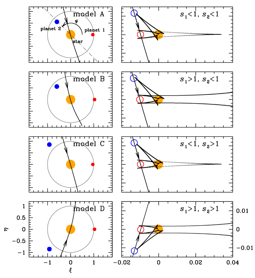
Figure 2.— Four possible geometries of the lens systems. Each of the left panels shows the relative positions of the two planets with respect to the host star. Coordinates are centered at the position of the host star and all lengths are normalized by the Einstein radius. The circle with a radius 1.0 represents the Einstein ring. Also marked is the trajectory of the source star (a curve with an arrow). Right panels show an enlarged view of the central region around the host star. The cuspy feature represents the caustics. The two small empty dots represent the source star at the moments of the major perturbations. The size of the dots is scaled to represent the source size.

We find that consideration of the parallax effect is needed to precisely describe the light curve. The parallax effect is caused by the change of the observer’s position due to the orbital motion of the Earth around the Sun during the event (Gould, 1992). For OGLE-2012-BLG-0026, the event time scale is of order 90 days, which comprises a significant fraction of the Earth’s orbital period, and thus parallax can affect the lensing light curve. We therefore introduce two additional parallax parameters of $\pi_{{\rm E},N}$ and $\pi_{{\rm E},E}$, which represent the two components of the lens parallax vector $\mbox{\boldmath$\pi$}_{\rm E}$ projected on the sky in the north and east equatorial coordinates, respectively. The direction of the parallax vector corresponds to the lens-source relative motion in the frame of the Earth. The size of the parallax vector is defined as the ratio of Earth’s orbit to the physical Einstein radius projected on the observer plane, i.e. $\pi_{\rm E}={\rm AU}/[\theta_{\rm E}/(D_{\rm L}^{-1}-D_{\rm S}^{-1})]$, where $D_{\rm L}$ and $D_{\rm S}$ are the distances to the lens and source star, respectively. We find that the parallax effect improves the fit by $\Delta\chi^{2}\sim 240$. We note that “terrestrial” parallax effect due to non-cospatial observatories on the Earth (Gould et al., 2009) is not detected since the separation between the 2 observatories covering the caustic crossings (Auckland and PEST) is not big enough.

For high-magnification events, planets described by $(s,q)$ and $(s^{-1},q)$ induce nearly identical caustics and thus nearly identical light curves (Griest & Safizadeh, 1998). This is known as the close/wide degeneracy in lensing light curves. We, therefore, investigate other solutions with initial values of the projected separations based on the first solution. From this search, we find 4 sets of solutions with ($s_{1}<1$, $s_{2}<1$), ($s_{1}>1$, $s_{2}<1$), ($s_{1}<1$, $s_{2}>1$), and ($s_{1}>1$, $s_{2}>1$). We denote the individual models as “A”, “B”, “C”, and “D”.

If the source were exactly on the ecliptic, it would exactly obey the “ecliptic degeneracy”, which takes $(u_{0},\alpha,\pi_{{\rm E},\perp})\rightarrow-(u_{0},\alpha,\pi_{{\rm E},\perp})$ (Skowron et al., 2011). Here $\pi_{{\rm E},\perp}$ is the component of $\mbox{\boldmath$\pi$}_{\rm E}$ perpendicular to the ecliptic at the projected position of the Sun at $t_{0}$, which in the present case is almost exactly north. OGLE-2012-BLG-0026 lies $<4^{\circ}$ [$(\lambda,\beta)_{J2000}=(264.28^{\circ},-3.83^{\circ})$] from the ecliptic. Hence it is not surprising that we find almost perfect ecliptic degeneracy for all four solutions, with $\Delta\chi^{2}\lesssim 1$. We do not show these redundant solutions.

In principle, one can detect lens orbital motion, and even if not, tangential orbital motion can be degenerate with $\pi_{{\rm E},\perp}$ (Batista et al., 2011), which would degrade the parallax measurement. We fit for all possible orientations of co-planar circular orbital motion (hence two additional parameters to define the orbit plane). However, we find, first that there is no improvement in the fit ($\Delta\chi^{2}\lesssim 1$), and second that there is no degeneracy with $\pi_{{\rm E},\perp}$. We therefore do not further consider orbital motion.

In Table 2, we present the four solutions. In Figure 2, we also present the geometries of the lens system corresponding to the individual solutions. We find that both planets responsible for the perturbation are located near the Einstein ring of the host star. The negative perturbation was produced by the passage of the source trajectory on the backside of the central caustic induced by a planet located almost on the Einstein ring of the host star, while the positive perturbation was produced when the source passed the sharp front tip of the arrowhead-shaped central caustic induced by another planet located at a position slightly away from the Einstein ring. The position angle of the second planet with respect to the first planet is $\psi\sim 220^{\circ}$. We note that although the close/wide degeneracy causes ambiguity in the star-planet separation, the mass ratios of the two degenerate solutions are similar to each other. We find that the mass ratios are $q_{1}\sim 1.3\times 10^{-4}$ and $q_{2}\sim 7.8\times 10^{-4}$.

4. Physical Parameters

The combined measurements of the angular Einstein radius and the lens parallax enable an estimate of the lens mass and distance. With these values, the mass and distance are determined by $M=\theta_{\rm E}/(\kappa\pi_{\rm E})$ and the $D_{\rm L}={\rm AU}/(\pi_{\rm E}\theta_{\rm E}+\pi_{\rm S})$, where $\kappa=4G/(c^{2}{\rm AU})$ and $\pi_{\rm S}={\rm AU}/D_{\rm S}$ is the parallax of the source star (Gould, 2000). By modeling the Galactic bulge as a bar, the distance to the source star is estimated by $D_{\rm S}=D_{\rm GC}(\cos\ell+\sin\ell\cos\phi/\sin\phi)$, where $D_{\rm GC}=8.16$ pc is the Galactocentric distance (Nataf et al., 2012), $\ell=0.195^{\circ}$ is the Galactic longitude of the source star, $\phi=40^{\circ}$ is the bar orientation angle with respect to the line of sight. This results in $D_{\rm S}=8.13$ kpc, corresponding to $\pi_{\rm S}=0.123$ mas.

The Einstein radius is given by $\theta_{\rm E}=\theta_{\star}/\rho_{\star}$ where $\theta_{\star}$ is the angular radius of the source, which we evaluate from its de-reddened color $(V-I)_{0}$ and brightness $I_{0}$ using an instrumental color-magnitude diagram (Yoo et al., 2004). We first measure the offset $\Delta[(V-I),I]=(-0.07,2.79)$ mag of the source from the clump, whose de-reddened position is known independently, $[(V-I),I]_{0,\rm c}=(1.06,14.45)$ mag (Bensby et al., 2011; Nataf et al., 2012). This yields the de-reddened color and magnitude of the source star $[(V-I),I]_{0,{\rm S}}=(0.99,17.23)$ mag. Thus the source is a bulge subgiant. Note that Bensby et al. (2013) estimate a very similar color $(V-I)_{0}=1.00$ mag based on a high-resolution VLT spectrum taken at high magnification. Figure 3 shows the locations of the source star and the centroid of the giant clump in the color-magnitude diagram that is constructed based on the OGLE data. Once the de-reddened $V-I$ color of the source star is measured, it is translated into $V-K$ color by using the $V-I$ versus $V-K$ relations of Bessell & Brett (1988) and then the angular source radius is estimated by using the relation between the $V-K$ color and the angular radius given by Kervella et al. (2004). The measured angular source radius is $\theta_{\star}=1.55\pm 0.13\ {\mu}{\rm as}$. Then, the Einstein radius is estimated as $\theta_{\rm E}=0.91\pm 0.09$ mas.

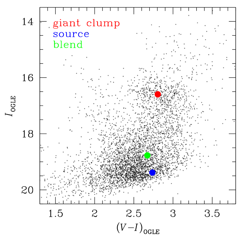
Figure 3.— Locations of the source star and blend in the color-magnitude diagram. Also marked is the position of the giant clump centroid that is used to calibrate the color and magnitude of the lensed star. Black dots are stars in the field where the source star is located.

In Table 1, we list the physical parameters of the planetary system determined based on model D, which provides the best fit. Other models are similar. According to the estimated mass of $\sim 0.82\ M_{\odot}$, the host star of the planets is a G-type main sequence. The individual planets have masses of $\sim 0.11\ M_{\rm J}$ and $0.68\ M_{\rm J}$. Their projected separations are $\sim$ 3.8 AU and 4.6 AU, respectively, and thus both planets are located well beyond the snow line 1.8 – 2.4 AU of the host star. The planetary system is located at a distance $\sim$ 4.1 kpc from the Earth toward the Galactic bulge direction.

To be noted is that the blend is likely to be the lens itself. Blended light refers to the extra light coming from stars other than the lensed star. The source of blended light can be unresolved stars located close to the lensed star or the lens itself. The fraction of blended light among total observed light is measured from modeling of the light curve. Considering the distance to the lens $\sim 4.1$ kpc, one can assume that the lens and the source experience roughly the same amount of reddening and extinction. Under this approximation, the estimated de-reddened color and brightness of the blend determined with the reference of the giant clump are $(V-I,I)_{0,{\rm b}}=(0.93,16.62)$ mag. Then, under the assumption that the blend is the lens combined with the distance modulus $\sim$ 13.05 mag to the lens, the estimated absolute magnitude of the blend is $M_{I,{\rm b}}\sim 3.6$ mag. Then, the color and the absolute magnitude of the blend roughly agree with the color $(V-I)_{0}\sim 0.9$ mag and the absolute magnitude $M_{I}\sim 4.2$ mag of a G5V star, that corresponds to the lens, suggesting that blended light comes from the host star. Moreover, from difference imaging the magnified and unmagnified images, we find that the blend and source have identical positions within measurement error ($\sim 50$ mas), further tightening the identification of the blend with the lens.

This identification opens many possibilities for future follow-up observations. AO imaging could confirm and refine the host star flux measurement by isolating it from fainter ambient stars. At $I=19$ mag, the host is bright enough to obtain a spectroscopic metallicity measurement, which would be the first for a microlensing planet host. Finally, late-time astrometry could improve the mass and distance determinations by refining the $\theta_{\rm E}$ measurement from the magnitude of the proper-motion vector (Alcock et al., 2001) and refining the $\mbox{\boldmath$\pi$}_{\rm E}$ measurement from its direction (Ghosh et al., 2004).

Table 1Physical Parameters

parameter	quantity
mass of the host star	0.82 $\pm$ 0.13 $M_{\odot}$
mass of the first planet	0.11 $\pm$ 0.02 $M_{\rm J}$
mass of the second planet	0.68 $\pm$ 0.10 $M_{\rm J}$
projected separation to the first planet	3.82 $\pm$ 0.30 AU
projected separation to the second planet	4.63 $\pm$ 0.37 AU
distance to the planetary system	4.08 $\pm$ 0.30 kpc

Table 2Lensing Parameters

parameters	model A	model B	model C	model D
$\chi^{2}/{\rm dof}$	2689.7/2667	2681.0/2667	2680.8/2667	2674.4/2667
$t_{0}$ (HJD’)	5991.52 $\pm$ 0.01	5991.52 $\pm$ 0.01	5991.52 $\pm$ 0.01	5991.52 $\pm$ 0.01
$u_{0}$	-0.0094 $\pm$ 0.0001	-0.0097 $\pm$ 0.0001	-0.0094 $\pm$ 0.0001	0.0092 $\pm$ 0.0001
$t_{\rm E}$ (days)	92.45 $\pm$ 1.08	89.21 $\pm$ 0.17	92.85 $\pm$ 1.11	93.92 $\pm$ 0.58
$s_{1}$	0.957 $\pm$ 0.001	1.034 $\pm$ 0.001	0.957 $\pm$ 0.001	1.034 $\pm$ 0.001
$q_{1}$ ($10^{-4}$)	1.32 $\pm$ 0.02	1.37 $\pm$ 0.01	1.30 $\pm$ 0.02	1.30 $\pm$ 0.01
$s_{2}$	0.812 $\pm$ 0.004	0.819 $\pm$ 0.004	1.257 $\pm$ 0.006	1.254 $\pm$ 0.006
$q_{2}$ ($10^{-4}$)	7.97 $\pm$ 0.26	7.84 $\pm$ 0.25	8.04 $\pm$ 0.25	7.84 $\pm$ 0.21
$\alpha$	1.283 $\pm$ 0.001	1.284 $\pm$ 0.001	1.284 $\pm$ 0.001	4.999 $\pm$ 0.001
$\psi$	2.389 $\pm$ 0.002	2.387 $\pm$ 0.001	2.391 $\pm$ 0.001	3.891 $\pm$ 0.001
$\rho_{\star}$ ($10^{-3}$)	1.73 $\pm$ 0.02	1.81 $\pm$ 0.01	1.72 $\pm$ 0.02	1.72 $\pm$ 0.01
$\pi_{{\rm E},N}$	-0.029 $\pm$ 0.054	-0.097 $\pm$ 0.012	0.001 $\pm$ 0.028	-0.072 $\pm$ 0.051
$\pi_{{\rm E},E}$	0.123 $\pm$ 0.009	0.137 $\pm$ 0.003	0.123 $\pm$ 0.005	0.114 $\pm$ 0.004

Note. — HJD’=HJD-2450000.

References

- Alard & Lupton (1998) Alard, C., & Lupton, R. 1998, ApJ, 503, 325
- Albrow et al. (2009) Albrow, M. D., Horne, K., Bramich, D. M, et al. 2009, MNRAS, 397, 2099
- Alcock et al. (2001) Alcock, C., Allsman, R. A., Alves, D. R., et al. 2001, Nature, 414, 617
- Batista et al. (2011) Batista, V., Gould, A., Dieters, S., et al. 2011, A&A, 529, 102
- Bennett et al. (2010) Bennett, D. P., Rhie, S. H., Nikolaev, S., et al. 2010, ApJ, 713, 837
- Bensby et al. (2011) Bensby, T., Adén, D., Melédez, J., et al. 2011, A&A, 533, 134
- Bensby et al. (2013) Bensby, T., Yee, J. C., Feltzing, S., et al. 2012, A&A, in press
- Bessell & Brett (1988) Bessell, M. S., & Brett, J. M. 1988, PASP, 100, 1134
- Gaudi et al. (1999) Gaudi, B. S., Naber, R. M., & Sackett, P. D. 1998, ApJ, 502, L33
- Gaudi et al. (2008) Gaudi, B. S., Bennett, D. P., Udalski, A., et al. 2008, Science, 319, 927
- Ghosh et al. (2004) Ghosh, H., DePoy, D. L., Gal-Yam, A., et al. 2004, ApJ, 615, 450
- Gould (1992) Gould, A. 1992, ApJ, 392, 442
- Gould (2000) Gould, A. 2000, ApJ, 542, 785
- Gould et al. (2009) Gould, A., Udalski, A., Monard, B., et al. 2009, ApJ, 698, L147
- Gould & Loeb (1992) Gould, A., & Loeb, A. 1992, ApJ, 396, 104
- Griest & Safizadeh (1998) Griest, K., & Safizadeh, N. 1998, ApJ, 500, 37
- Han (2005) Han, C. 2005, ApJ, 629, 1102
- Han (2009) Han, C. 2009, ApJ, 691, L9
- Han & Gaudi (2008) Han, C., & Gaudi, B. S. 2008, ApJ, 689, 43
- Ida & Lin (2004) Ida, S., & Lin, D. N. C. 2004, ApJ, 604, 388
- Ida & Lin (2005) Ida, S., & Lin, D. N. C. 2005, ApJ, 626, 1045
- Kennedy & Kenyon (2008) Kennedy, G. M., & Kenyon, S. J. 2008, ApJ, 673, 502
- Kervella et al. (2004) Kervella, P., Thévenin, F., Di Folco, E., & Ségransan, D. 2004, A&A, 426, 297
- Mao & Paczyński (1991) Mao, S., & Paczyński, B. 1991, ApJ, 374, L37
- Nataf et al. (2012) Nataf, D. M., Gould, A., Fouqué, P., et al. 2012, ApJ, submitted (arXiv:1208.1263)
- Pollack et al. (1996) Pollack, J. B., Hubickyj, O., Bodenheimer, P., Lissauer, J. J., Podolak, M., & Greenzweig, Y. Icarus, 124, 62
- Raymond et al. (2007) Raymond, S. N., Quinn, T., & Lunine, J. I. 2007, Astrobiology, 7, 66
- Schechter et al. (1993) Schechter, P. L., Mateo, M., & Saha, A. 1993, PASP, 105, 1342
- Skowron et al. (2011) Skowron, J., Udalski, A., Gould, A., et al. 2011, ApJ, 738, 87S
- Udalski (2003) Udalski, A. 2003, Acta Astron., 53, 291
- Woźniak (2000) Woźniak, P. R. 2000, Acta Astron., 50, 421
- Yoo et al. (2004) Yoo, J., DePoy, D. L., Gal-Yam, A., et al. 2004, ApJ, 603, 139