Collisionless shocks in a partially ionized medium.
II. Balmer emission

Abstract

Strong shocks propagating into a partially ionized medium are often associated with optical Balmer lines. This emission is due to impact excitation of neutral hydrogen by hot protons and electrons in the shocked gas. The structure of such Balmer-dominated shocks has been computed in a previous paper Blasi et al. (2012), where the distribution function of neutral particles was derived from the appropriate Boltzmann equation including coupling with ions and electrons through charge exchange and ionization. This calculation showed how the presence of neutrals can significantly modify the shock structure through the formation of a neutral-induced precursor ahead of the shock. Here we follow up on our previous work and investigate the properties of the resulting Balmer emission, with the aim of using the observed radiation as a diagnostic tool for shock parameters. Our main focus is on Supernova Remnant shocks, and we find that, for typical parameters, the H$\alpha$ emission typically has a three-component spectral profile, where: 1) a narrow component originates from upstream cold hydrogen atoms, 2) a broad component comes from hydrogen atoms that have undergone charge exchange with shocked protons downstream of the shock, and 3) an intermediate component is due to hydrogen atoms that have undergone charge exchange with warm protons in the neutral-induced precursor. The relative importance of these three components depends on the shock velocity, on the original degree of ionization and on the electron-ion temperature equilibration level. The intermediate component, which is the main signature of the presence of a neutral-induced precursor, becomes negligible for shock velocities $\buildrel<\over{{}_{\sim}}1500$ km/s. The width of the intermediate line reflects the temperature in the precursor, while the width of the narrow one is left unaltered by the precursor. In addition, we show that the profiles of both the intermediate and broad components generally depart from a thermal distribution, as a consequence of the non equilibrium distribution of neutral hydrogen. Finally, we show that a significant amount of Balmer emission can be produced in the precursor region if efficient electron heating takes place.

1. Introduction

It has been shown Chevalier & Raymond (1978) that optical spectra dominated by H$\alpha$ and other Balmer lines, as observed in some historical Supernova Remnants (SNRs), may arise when an astrophysical shock propagates through a partially ionized medium.

The Balmer emission, observed from these so-called Balmed-dominated shocks, provides a powerful diagnostic tool to investigate the conditions existing in the shock vicinity. The H$\alpha$ lines typically show two components, resulting from excitation of neutral hydrogen due to the interaction with hot protons and electrons in the shocked gas: a narrow-line component, whose width is characteristic of the cold interstellar medium and that has been explained as the result of direct excitation of neutral hydrogen atoms; and a much broader component, associated to a second population of hydrogen atoms, created by charge-exchange (CE) processes between the cold, still unshocked hydrogen and the shocked protons. These hot atoms can be produced in an excited state or can be excited by subsequent collisions with protons or electrons. Hence the line width of the broad component traces the thermal velocity of shocked protons and can be used to infer the shock velocity. Combining this estimate with proper motion measurements, one can estimate the distance to the object.

Besides the shock speed, Balmer lines also represent a unique tool to investigate the plasma physics of collisionless shocks. If both narrow and broad components are detected, the relative intensity of the two lines can be used to infer the ratio of electron-to-ion temperature just behind the shock, providing information on the electron-ion equilibration mechanisms Ghavamian et al. (2007); van Adelsberg et al. (2008).

One of the most intriguing aspects of Balmer emission is related to the possibility of using the line shape and its spatial profile to check the efficiency of SNR shocks in accelerating cosmic rays (CRs). If CR acceleration is taking place in an efficient way, then the widths of both the narrow and broad line may be affected. In fact, when a sizable fraction of the ram pressure is channeled into non-thermal particles, the plasma temperature behind the shock is expected to be lower, and this should reflect in a narrower width of the broad H$\alpha$ line. On the other hand efficient particle acceleration also leads to the formation of a CR-induced precursor upstream, which heats the ionized plasma before the shock. If the precursor is large enough, CE can occur upstream leading to a broader narrow Balmer line. Remarkably, both signatures seem to have been observed in Balmer-dominated shocks. For example Helder et al. (2009) combined proper motion measurements of the shock and broad H$\alpha$ line width for the remnant RCW 86 to demonstrate that the temperature behind the shock is too low, thereby concluding that a sizable fraction of the energy is being channelled into cosmic rays. However, qualitatively similar features can also arise from different physical processes. Therefore their observation can only be turned into reliable information on the shock properties after a quantitative physical description of the phenomenon is provided.

The basic theory of collisionless shocks in the presence of neutral particles was first developed by Chevalier & Raymond (1978) and Chevalier et al. (1980) and further refined by Smith et al. (1991) and Ghavamian et al. (2001). These papers were however characterized by similar rather important limitations, mainly due to the assumption that the distribution functions of both populations of neutrals are Maxwellians. In fact, the main difficulty in describing the structure of a collisionless shock propagating in a partially ionized medium is that neutrals have no time to reach thermalization and cannot be treated as a fluid. Steps forward in relaxing the fluid assumption have been made by Heng & McCray (2007) and van Adelsberg et al. (2008) which considered the effect of multiple CE events on the distribution function of hot neutrals. However these authors limit their calculations to the region downstream of the shock, and consider only the volume integrated distributions.

A proper description of the effects of the interactions between neutrals and ions on the neutral distribution function requires a fully kinetic approach. This approach has been implemented by Blasi et al. (2012) (hereafter, Paper I) where we derived simultaneously the neutral distribution function and the hydrodynamic quantities for ions (which are, instead, treated as a fluid), both upstream and downstream of the shock, by solving a Boltzmann equation including CE and ionization terms. The main result of Paper I is that of providing a mathematical and physical description of what we call the neutral return flux: when fast, cold neutrals undergo CE interactions with the slower hot ions downstream of the shock, some fraction of the resulting hot neutrals can cross the shock and move upstream. The relative velocity between these hot neutrals and the upstream ions triggers the onset of CE and ionization interactions that lead to the heating and slowing down of the ionized component of the upstream fluid. The system then tends to develop a shock precursor, in which the fluid velocity gradually decreases from its value at upstream infinity, and even more important, the temperature of ions in the upstream region increases as a result of the energy and momentum deposition of returning neutrals.

The existence of a neutral return flux from downstream to upstream was previously mentioned by Smith et al. (1994) and Hester et al. (1994) as a possible way to explain the anomalous width of narrow Balmer lines observed in some SNRs (see e.g. Sollerman et al., 2003), but no explicit calculation was carried out.

The width of such lines is in the 30-50 km/s range, implying a pre-shock temperature around 25000-50000 K. If this were the ISM equilibrium temperature there would be no atomic hydrogen, implying that the pre-shock hydrogen is heated by some form of shock precursor in a region that is sufficiently thin so that collisional ionization equilibrium cannot be established before the shock. Several mechanisms have been proposed to explain the broadening of the narrow line (see Heng, 2009, for a review), but most of them can be ruled out on theoretical grounds, leaving a CR precursor and/or a neutral precursor as the most probable origin.

A first attempt at investigating the broadening of the narrow line component induced by the neutral precursor was made by Lim & Raga (1996), using a simplified Boltzmann equation for neutrals in one dimension in both physical and velocity space. The calculations were carried out for a shock speed of $225$ km/s, and varying the initial ionization fraction from 0.5 to 0.99. The narrow line width does not show any appreciable change due to the return flux.

In the present work we use the theory developed in Paper I and calculate the profile of Balmer line emission in the presence of neutral return flux. In particular we show that the neutral return flux is responsible for the emission of a third intermediate line component, in addition to the narrow and broad ones. This intermediate line is produced by hydrogen atoms that have undergone CE with warm protons in the neutral precursor. Interestingly, there are observations which suggest the existence of such intermediate component Ghavamian et al. (2000), although the results might also be due to projection effects since the emission region is morphologically rather complex. At the present time, spectral and spatial information are not sufficient to disentangle the physical effect that we describe here from geometrical and projection effects which could modify the line profiles. We also show that the neutral-induced precursor is not able to broaden the width of narrow H$\alpha$ line, confirming the first finding of Lim & Raga (1996).

The paper is organized as follows: in §2 we summarize the kinetic approach developed in Paper I and use it to describe the shock structure in the presence of neutrals. We improve on previous work by both adding electrons in the shock dynamics and including their contribution to the ionization of neutrals. In §3 we write down the basic equations for the calculation of the Balmer line emission and in §4 we illustrate the main results in terms of spatial profiles of the total emission, of line profile, as well as line intensity ratios. We also compare theoretical profiles with profiles obtained by simulated observations, in order to derive the observational requirements necessary in order to be able to detect the intermediate component, and deviations from gaussianity in general. We conclude in §5.

2. Physical model

The basic model we consider consists of a plane-parallel shock with velocity $V_{sh}$ that propagates into a partially ionized proton-electron plasma along the $z$ direction, with a given fraction of neutral hydrogen at upstream infinity. We neglect the presence of helium and other heavier chemical elements.

Protons and electrons are assumed to behave as fluids with temperatures $T_{i}(z)$ and $T_{e}(z)$, respectively, with the same bulk velocity, $v_{i}(z)=v_{e}(z)$, and the same number density, $n_{i}(z)=n_{e}(z)$. Their distribution functions, $f_{i}(\vec{v},z)$ and $f_{e}(\vec{v},z)$, are assumed to be Maxwellian at each position $z$. Neutral hydrogen interacts with protons and electrons through CE and ionization. The hydrogen distribution function, $f_{N}(\vec{v},z)$, can be described using the Boltzmann equation

$$\frac{\partial f_{N}}{\partial t}+\vec{v}\cdot\nabla f_{N}=\beta_{N}f_{i}-\beta_{i}f_{N}-\beta_{e}f_{N},$$ (1)

where the collision terms $\beta_{k}f_{l}$ represent the interaction (due to CE and ionization) between the species $k$ and $l$. The interaction rate $\beta_{k}$ is formally written as

$$\beta_{k}(\vec{v},z)=\int d^{3}w\,v_{rel}\,\sigma(\vec{v}_{rel})f_{k}(\vec{w},z)\,,$$ (2)

where $v_{rel}=|\vec{v}-\vec{w}|$ and $\sigma$ is the cross section for the interaction process. More precisely, $\beta_{N}$ is the rate of CE of an ion that becomes a neutral, $\beta_{i}$ is the rate of CE plus ionization of a neutral due to collisions with protons, while $\beta_{e}$ is the ionization rate of neutrals due to collisions with electrons. Eq. (1) is used to calculate $f_{N}$ starting from the distribution of charged species (protons and electrons), under the assumption of stationarity ($\partial f_{N}/\partial t=0$).

The dynamics of protons and electrons coupled with neutrals can be described very generally through conservation equations of mass, momentum and energy:

$$\frac{\partial}{\partial z}\left[(\rho_{i}+\rho_{e})v_{i}+F_{mass}\right]=0\,,$$ (3)

$$\frac{\partial}{\partial z}\left[(\rho_{i}+\rho_{e})v_{i}^{2}+P_{i}+P_{e}+F_{mom}\right]=0\,,$$ (4)

$$\frac{\partial}{\partial z}\left[\frac{1}{2}(\rho_{i}+\rho_{e})v_{i}^{3}+\frac{\gamma_{g}(P_{i}+P_{e})v_{i}}{\gamma_{g}-1}+F_{en}\right]=0\,,$$ (5)

where $F_{mass}=m_{H}\int d^{3}vv_{\parallel}f_{N}$, $F_{mom}=m_{H}\int d^{3}vv_{\parallel}^{2}f_{N}$ and $F_{en}=m_{H}/2\int d^{3}vv_{\parallel}(v_{\parallel}^{2}+v_{\perp}^{2})f_{N}$ are respectively the fluxes of mass, momentum and energy of neutrals along the $z$ direction. Usually the dynamical role of electrons is neglected due to their small mass. However, collective plasma processes could contribute to equilibrate electron and proton temperatures to some level. If this equilibration is very efficient, then the electron pressure can no longer be neglected and the total gas pressure needs to include both proton and electron contributions, namely $P_{g}=P_{i}+P_{e}=P_{i}(1+\beta)$, where $\beta(z)\equiv T_{e}/T_{i}$ is the electron to proton temperature ratio and is taken as a free parameter.

The solution of Eqs.(1)-(5) is described in detail in Paper I. The only difference here is the presence of electrons, which has been previously neglected because it does not affect the shock dynamics, unless $T_{e}\sim T_{i}$. The importance of introducing the electron contribution in this context comes from the fact that Balmer emission is very sensitive to both $T_{e}$ and $T_{i}$ Heng & McCray (2007); van Adelsberg et al. (2008). Therefore, even very partial equilibration can produce observational consequences in the line emission, as we show in §4.

The level of electron-ion equilibration is one of the open questions in collisionless shock physics and H$\alpha$ observations present us with a unique tool to investigate this aspect. Theoretically the equilibration process is far from being understood and anything between total absence of interaction and full equilibration has been proposed (see Rakowsky, 2005, for a review). Moreover the electron-ion equilibration level is expected to change between upstream and downstream of the shock, because the plasma conditions in these two regions are totally different in terms of temperature and turbulence properties. As a consequence, we distinguish between upstream and downstream using two separate parameters, $\beta_{up}$ and $\beta_{down}$, respectively.

We stress that a crucial assumption of our calculation is that new protons produced at position $z$ by CE and ionization instantly thermalize with other protons. As discussed in Paper I, such an assumption, which is especially important in the upstream region, is rather delicate: protons might isotropize and yet not thermalize with the rest of protons in the plasma. A dedicated effort using numerical particle simulations should be used to address this important issue.

In principle, the dynamics of electrons in the upstream region could also be affected by electrons ejected due to the ionization of neutrals that have returned upstream. This effect can however be neglected for the calculation of Balmer lines: in Paper I we showed that the fraction of returning neutrals is $\buildrel<\over{{}_{\sim}}5\%$. Let us assume that all these neutrals are ionized in the upstream region. To a good approximation, stripped electrons can be expected to have the same velocity of their parent atoms, which, in turn, have a mean velocity of the order of the downstream proton thermal speed. Hence the temperature of stripped electrons is $T_{e,in}\simeq 3/8V_{sh}^{2}m_{e}/k_{B}\approx 6.2\times 10^{5}(V_{sh}/5000\rm km/s)^{2}$K. Now, assuming that the newly generated electrons reach equilibrium with preexisting electrons, the final temperature is of the order of $(n_{0}T_{0}+n_{in}T_{in})/(n_{0}+n_{in})\approx 2.5\times 10^{4}$K, where we use $V_{sh}=5000$ km/s and an initial ionization fraction of 50%. This temperature is too low to be relevant for Balmer emission. In fact, electrons can contribute only if their velocity is $\buildrel>\over{{}_{\sim}}2000$ km/s, namely if $T_{e}\buildrel>\over{{}_{\sim}}10^{5}$K.

3. Calculation of Balmer line emission

Once the distribution functions of hydrogen, protons and electrons are known at each position, the calculation of line emission is quite straightforward, provided that the relevant cross sections are known. Here we concentrate on the Balmer H$\alpha$ line, which results from the hydrogen deexcitation from level $3s$ and $3d$ to $2p$ as well as from $3p$ to $2s$. The latter case is complicated by the fact that the $3p$ level can also decay into $1s$, producing Ly$\beta$ photons. Depending on the optical depth of the medium, these photons can either escape the system or be reabsorbed by ground-state hydrogen and eventually reemitted as H$\alpha$ photons. In the literature the optically thin and optically thick cases are usually labelled as Case A and Case B, respectively, and the total H$\alpha$ production rate is written as:

$$R_{H\alpha}=R_{H(3s)}+R_{H(3d)}+B_{3p,2s}R_{H(3p)}\,,$$ (6)

where $R_{H(3l)}$ is the production rate of hydrogen excited at level $3l$ and the factor $B_{3p,2s}$ is the fraction of transitions from $3p$ to $2s$, which is $\approx 0.12$ in the optically thin case (Case A) while it becomes unity in the optically thick case (Case B) van Adelsberg et al. (2008).

The conversion efficiency from Ly$\beta$ to $H\alpha$ photons depends on the shock speed, the electron-ion temperature ratio and the pre-shock ionization fraction. It was first computed by Chevalier et al. (1980), who found that in conditions appropriate for many Balmer dominated shocks the emission from cold hydrogen is generally optically thick while the emission from hot hydrogen is close to be optically thin. In this work, following that result, we adopt $B_{3p,2s}=0.12$ (1) for the emission produced by hot (cold) hydrogen.

In order to calculate the H$\alpha$ emission for both Case A and Case B, we need to compute the different production rates of hydrogen excited to the sublevels $3s$, $3p$ and $3d$. The excited hydrogen is mainly produced by two different processes: collisions with protons and electrons, and CE reactions leaving the hydrogen atom in an excited state. For the sake of clarity here we neglect further contributions due to collisions with helium. The production rate of $H(3l)$ at a fixed position $z$ reads:

$$R_{H(3l)}(\vec{v},z)=\int d^{3}w\,v_{rel}\,f_{H}(\vec{v},z)\times$$

$$\left[f_{i}(\vec{w},z)\,\sigma_{ex(i)}^{tot(3l)}(v_{rel})+f_{e}(\vec{w},z)\,\sigma_{ex(e)}^{tot(3l)}(v_{rel})\right]$$

$$+\int d^{3}w\,v_{rel}\,f_{i}(\vec{v},z)f_{H}(\vec{w},z)\,\sigma_{ce}^{tot(3l)}(v_{rel})\,.$$ (7)

Notice that the hydrogen distribution function $f_{H}$ includes only atoms at the ground level $1s$. In fact, collisional deexcitation can be neglected because it occurs on a typical time scale $\tau_{coll}\simeq(n_{i}\sigma_{coll}V_{sh})^{-1}\simeq 10^{7}{\rm sec}$ (for $n_{i}=1\,{\rm cm^{-3}}$ and $V_{sh}=1000\,{\rm km/s}$) which is much longer than spontaneous deexcitation, whose time scale (from state $n$ to state $m$) is $\tau=\hbar/\Delta E=4.8\times 10^{-15}(n^{-2}-m^{-2})\,{\rm sec}$. Hence atoms decay to the ground state before undergoing any further collision.

In Eq. (3) we use the total excitation and CE cross sections for the atomic sublevel $3l$, $\sigma_{ex}^{tot(3l)}$ and $\sigma_{ce}^{tot(3l)}$, which take into account the direct excitation processes, $1s\rightarrow 3l$, plus contributions coming from atoms excited to higher levels with $n>3$ that subsequently decay to the state $3l$. Formally this total cross section can be written in the following form:

$$\sigma^{tot(3l)}=\sum_{n^{\prime},l^{\prime}}^{\infty}\,B_{n^{\prime}l^{\prime},3l}\,\sigma_{1s\rightarrow n^{\prime}l^{\prime}}\,.$$ (8)

where $\sigma_{1s\rightarrow n^{\prime}l^{\prime}}$ is the cross section for excitation from the ground state to the level $n^{\prime}l^{\prime}$ and the $B_{n^{\prime}l^{\prime},nl}$ are the cascade matrix elements representing the probability that a hydrogen atom excited to state $n^{\prime}l^{\prime}$ will make a transition to state $nl$ (with $n<n^{\prime}$) via all cascade routes.

We treat CE, excitation and ionization between electrons, protons and hydrogen atoms using the cross sections of Barnett el al. (1990), Belkić et al. (1992), Janev & Smith (1993), Balança et al. (1998) and Harel et al. (1998). For some of these cross sections we adopt the fitting functions provided by Heng & Sunyaev (2008) and Tseliakhovich et al. (2012). At the time of writing, the CE cross sections for sublevels with different angular momentum states are known only up to the level $n=4$. We estimate that neglecting the contribution of higher levels entails an error around $5\%$ in the calculation of the total $\sigma_{ce}$, therefore in the following we ignore levels with $n>4$. Hence, for the CE process, the cross sections reduce to the following:

$$\sigma_{ce}^{tot(3s)} \simeq\sigma_{ce,1s\rightarrow 3s}+B_{4p,3s}\,\sigma_{ce,1s\rightarrow 4p}\,,$$ (9)

$$\sigma_{ce}^{tot(3d)} \simeq\sigma_{ce,1s\rightarrow 3d}+B_{4d,3d}\,\sigma_{ce,1s\rightarrow 4d}\,,$$ (10)

$$\sigma_{ce}^{tot(3p)} \simeq\sigma_{ce,1s\rightarrow 3p}+B_{4s,3p}\,\sigma_{ce,1s\rightarrow 4s}$$

$$\quad+B_{4d,3p}\,\sigma_{ce,1s\rightarrow 4d}\,,$$ (11)

where we use the values of $B_{4l^{\prime},3l}$ as listed by Heng & Sunyaev (2008) (see their Table 3). An identical approach is adopted to calculate the impact excitation by protons, restricted to levels 3 and 4. We adopt the impact excitation cross sections calculated by Balança et al. (1998) and Tseliakhovich et al. (2012) for the sublevels $3l$ and $4l$ respectively. Unfortunately these works provide cross sections only for a limited range of impact energies, 1–100 keV and 5–80 keV respectively, which means that the relative speed between protons and hydrogen atoms can be respectively in the range $[v_{1},v_{2}]=[438,4377]$ km/s and $[978,3914]$ km/s. Outside these velocity ranges we estimate the sublevel cross sections, $\sigma_{ex(i)}^{nl}$, using the total cross sections, $\sigma_{ex(i)}^{n}$ as taken from Janev & Smith (1993), in the following way:

$$\sigma_{ex(i)}^{nl}(v>v_{2})=\sigma_{ex(i)}^{n}(v)\frac{\sigma_{ex(i)}^{nl}(v_{2})}{\sigma_{ex(i)}^{n}(v_{2})}\left(1+\epsilon_{n}\right)\,,$$ (12)

where the coefficients $\epsilon_{n}$ are chosen in such a way as to have $\sum_{l}\sigma_{nl}(v_{1(2)})=\sigma_{n}(v_{1(2)})$, and their values are of the order of few percent. A similar approximation has been used also for $v<v_{1}$.

Also the impact excitation by electrons is limited to sublevels 3$l$ and 4$l$ and expressions similar to (9)-(11) hold for $\sigma_{ex(e)}^{tot(3l)}$ as well. In this case we use the cross sections provided by Bray & Stelbovics (1995), computed using the convergent close-coupling method. As for the previous case, the error in the total cross section produced by excluding higher excited levels is around 5%.

In order to compute the spatial emissivity profile of the H$\alpha$ emission we need to integrate Eq. (6) in the velocity directions orthogonal to the line of sight. From the observational point of view, most cases refer to shocks viewed edgewise because of limb brightening. In such cases, assuming a pure plane shock (i.e. neglecting curvature effects), the edge-wise emissivity profile results from the following integration:

$$F_{H\alpha}(z,v_{x})=\iint dv_{z}dv_{y}\left[R_{H(3s)}(z,\vec{v})\right.\qquad\qquad$$

$$\left.+R_{H(3d)}(z,\vec{v})+B_{3p,2s}R_{H(3p)}(z,\vec{v})\right]$$

$$=2\int_{-\infty}^{\infty}dv_{z}\int_{v_{x}}^{\infty}\frac{dv_{\bot}}{\sqrt{1-(v_{x}/v_{\bot})^{2}}}\quad\;\;$$

$$\left[R_{H(3s)}(z,v_{z},v_{\bot})+R_{H(3d)}(z,v_{z},v_{\bot})\right.$$

$$\left.+B_{3p,2s}R_{H(3p)}(z,v_{z},v_{\bot})\right]\,,$$ (13)

where $z$ is the direction of shock propagation, $x$ is the direction along the line of sight and $y$ is orthogonal to the $(x,z)$ plane. In the second equality we use $v_{\bot}\equiv({v_{x}^{2}+v_{y}^{2}})^{1/2}$. Starting from Eq. (3) we can obtain more useful integrated quantities, which can be directly compared with observations, namely the spatial emissivity profile, $\xi_{H\alpha}(z)$, the volume-integrated line profile, $\phi_{H\alpha}(v_{x})$, and the total line strength, $I_{H\alpha}$, respectively defined as

$$\xi_{H\alpha}(z)=\int_{-\infty}^{\infty}dv_{x}F_{H\alpha}(z,v_{x})\,,$$

$$\phi_{H\alpha}(v_{x})=\int_{-\infty}^{\infty}dz\,F_{H\alpha}(z,v_{x})\,,\;{\rm and}$$

$$I_{H\alpha}=\iint dv_{x}dz\,F_{H\alpha}(z,v_{x})\,.$$ (14)

In the next section we will investigate how these observables can be used to test the presence of a neutral-induced precursor and to infer the ambient parameters (as the ionization fraction, the shock speed and the electron-proton equilibration level).

4. Results

In this section we illustrate the main results of our kinetic calculation concerning the H$\alpha$ emission. It is well known that Balmer emission is highly sensitive to plasma density, shock velocity, initial degree of ionization and electron-ion equilibration level. Our aim is to illustrate how to disentangle different effects produced by these quantities. The main observable quantities are the spatial profile, the line profile and the relative intensity of the broad and narrow lines. Below we discuss the interpretation of these quantities and their relation with physical parameters, comparing our results with previous work.

For all cases discussed, we fix the temperature at upstream infinity to $10^{4}$K, because larger values are incompatible with the presence of neutral hydrogen, while for lower values the results do not change significantly. Also the total upstream numerical density is fixed to $n_{tot}=0.1{\rm cm^{-3}}$, while the plasma ionization fraction is assumed to be 50%, unless otherwise specified. We notice that the total density can be factorized out in Eqs.(1)-(5), hence a change in the total density only reflects in a change of the length scales of the problem, while all other quantities remain unchanged.

As we already pointed out, the electron-to-proton equilibration level, $\beta$, is expected to change between upstream and downstream of the shock, hence we use two independent parameters, $\beta_{up}$ and $\beta_{down}$, respectively. We will focus mainly on the two extreme cases of full equilibration (FE), where protons and electrons share the same temperature everywhere (i.e. $\beta_{up}=\beta_{down}=1$) and no equilibration at all (NE), which corresponds to the situation where electrons and protons do not interact at all. In the latter case the electron temperature is equal to $10^{4}$K in the entire upstream region and $\beta_{down}=m_{e}/m_{p}$ in the downstream. Intermediate equilibration cases will be also discussed.

4.1. Spatial emission

Figure 1.— Spatial emissivity profile of the H$\alpha$ line for $n_{tot}=0.1{\rm cm^{-3}}$, 50% ionization fraction and for different values of shock velocity, as specified in each panel. Two extreme cases of electron-ion temperature equilibration are shown: NE (upper panel) and FE (lower panel), i.e. $\beta_{up}=\beta_{down}=1$.

Figure 2.— Fraction of the total emissivity coming from the upstream as a function of shock velocity and for three different assumptions on the degree of electron-proton equilibration upstream ($\beta_{down}$ is fixed to 1 for all cases).

Figure 3.— Efficiency of the H$\alpha$ emission (i.e. number of photons emitted for each hydrogen atom crossing the shock) as a function of the shock velocity and for different degrees of electron-ion equilibration efficiency. The thick lines refer to the cases of non-equilibrium (solid), full equilibrium (dotted) and partial equilibrium with $\beta_{down}=0.1$ (dot-dashed). For these cases the plasma is assumed to be optically thin for Ly$\beta$ photons produced by hot hydrogen atoms, but optically thick for photons produced by cold hydrogen atoms. The thin lines, instead, show NE cases assuming a medium that is either optically thin (Case A) or optically thick (Case B) to Ly$\beta$ photons.

Fig. 1 shows the spatial emissivity profile, $\xi_{H\alpha}(z)$, for different shock velocities and for the two extreme assumptions for the electron-ion equilibration efficiency: the upper panel shows the NE case, while the lower panel shows the FE case. Interestingly, while in the former case the emission is produced only in the downstream, in the latter case a substantial fraction of the H$\alpha$ emission comes from the upstream. This fact is better illustrated in Fig. 2, where the fraction of total H$\alpha$ emission produced upstream is plotted as a function of shock velocity and for different values of electron-ion equilibration efficiency upstream (while $\beta_{down}$ is fixed to 1): the upstream emission has a peak when $V_{sh}$ is close to 2500 km/s and can reach $\sim 40\%$ of the total emission when $\beta_{up}=1$. Remarkably, even reducing $\beta_{up}$ down to 0.05, the upstream emission is still a non-negligible fraction of the total, being around $10\%$. For velocities $>2500$ km/s the upstream emission decreases monotonically because the heating produced by the neutral return flux becomes less efficient, as shown in Paper I (see its Fig. 6).

The H$\alpha$ emission produced upstream is clearly due to collisional excitation of hydrogen by electrons. In fact, this process has a threshold for $v_{rel}\simeq 2000$ km/s and peaks at $v_{rel}\simeq 3000$ km/s, hence when the electron temperature is larger than $\simeq 1.5\times 10^{5}$K the atomic level $n=3$ is easily excited and H$\alpha$ emission is produced. On the other hand, excitation produced upstream by protons is suppressed because, for a given common temperature, protons have a thermal speed $\sqrt{m_{e}/m_{p}}$ times lower than electrons; hence H$\alpha$ emission induced by proton collisions and CE becomes relevant only for $T_{p}\buildrel>\over{{}_{\sim}}\rm few\times 10^{7}$K. The heating induced by the neutral return flux may lead to such ion temperatures upstream, but only very close to the shock, on spatial scales that are too small to affect the H$\alpha$ emission.

From Fig. 1 we can see that H$\alpha$ emission seems to increase with increasing shock velocity. This is a consequence of the fact that the production efficiency of H$\alpha$-photons is almost constant at high $V_{sh}$. This is shown in Fig. 3 where we plot the efficiency of H$\alpha$ emissivity, defined as the number of H$\alpha$ photons emitted per hydrogen atom crossing the shock, namely $\epsilon=I_{H\alpha}/(V_{sh}n_{H,0})$, where $n_{H,0}$ is the hydrogen number density at upstream infinity. In Fig. 3 several cases are shown: the solid and dotted thick lines refer to NE and FE cases respectively, while the dot-dashed thick line refers to an intermediate case (NE upstream and partial equilibrium downstream with $\beta_{down}=0.1$). For all these three cases we assumed that the plasma is optically thin to Ly$\beta$ emission from hot hydrogen atoms (Case A) and optically thick to Ly$\beta$ emission from cold hydrogen (Case B) as discussed at the beginning of §3. In order to compare our results with previous work, we also plot the cases where the plasma is optically thin or optically thick for both the hot and the cold hydrogen emission, but only for the NE case.

These latter two cases can be compared with the estimated efficiency provided by Chevalier & Raymond (1978) who give $\epsilon_{A}=0.048$ and $\epsilon_{B}=0.27$, independently of the shock velocity. We note that while $\epsilon_{B}$ is quite close to our finding, especially for high shock speed, the value of $\epsilon_{A}$ is about a factor two smaller than our result. The discrepancy is probably due to the fact that the excitation cross sections used at that time were not very accurate.

4.2. H$\alpha$ line profile

Let us now analyze the shape of H$\alpha$ lines. Fig. 4 shows the volume-integrated line profiles, $\phi_{H\alpha}(v_{x})$, for several values of the shock velocity, for both NE (upper panel) and FE (lower panel) cases. Several comments are in order. The first point to note is that $\phi_{H\alpha}$ cannot be described, in general, by only two Gaussian-like components, as usually assumed in the literature. Besides the usual narrow and broad components, we clearly see the presence of a third intermediate component whose typical width is about few hundreds km/s. This intermediate component is a direct consequence of the existence of the neutral-induced precursor. In fact, as we showed in Paper I, the neutral return flux can heat upstream protons up to a temperature $\sim 10^{6}-10^{7}$K. Hence hydrogen atoms that undergo CE upstream with these warm protons can produce H$\alpha$ emission with a typical width of $\sim 100$ km/s. This picture also suggests that the intermediate component should have a non-Gaussian profile, because it contains contributions from hydrogen populations at different locations in the precursor, which have different temperatures.

This physical interpretation of the intermediate component is supported by the fact that its intensity, with respect to the narrow line, increases or decreases according to the temperature and length of the neutral precursor. For example, in Fig. 5 we show the effect of increasing the initial neutral fraction from 1% to 50%. We see that the intermediate component becomes more prominent as the neutral fraction increases: this is a consequence of the fact that the heating induced upstream by the neutral return flux increases. A similar behaviour occurs when changing the shock speed. In Paper I we showed that the upstream temperature has a maximum for $V_{sh}\simeq 2000$ km/s and decreases for smaller and larger speeds. The same happens for the emission of the intermediate component with respect to the narrow one (see Figs. 8 and 9).

Figure 4.— Volume-integrated H$\alpha$ emission for different values of the shock velocity. The upper and lower panels show the cases NE and the FE cases, respectively. The values of total density and ionization fraction are the same as in Fig. 1. The small boxes show a zoom for small values of $v_{x}$, aimed at emphasizing the shape of the narrow and intermediate lines.

Figure 5.— Volume-integrated H$\alpha$ emission for three different values of upstream ionization fraction.

The variation of electron-ion equilibration efficiency also considerably affects the line profile. In Fig. 6 we plot $\phi_{H\alpha}$ for a fixed shock speed and for different values of $\beta_{down}$. When $\beta_{down}$ increases, a decreasing of the broad emission is observed: this occurs because electrons contribute to ionize hot hydrogen atoms. Also the width of the broad component decreases because a fraction of the protons’ thermal energy is transferred to electrons, hence the proton temperature decreases. The narrow component, on the other hand, is only slightly affected by variations of $\beta_{down}$. Its intensity increases when $\beta_{down}$ goes from $m_{e}/m_{p}$ up to $\sim 0.01$, while for larger values it remains constant. In Fig. 6 we only consider the effect of electron-ion equilibration downstream, while the electron temperature upstream is taken constant and equal to $10^{4}$K. The effect of electron heating upstream can be appreciated by looking at Fig. 7, where we plot separately the volume-integrated emission from upstream and downstream assuming FE downstream, but distinguishing the NE and the FE cases upstream. The FE case shows that the total upstream emission is comparable to the downstream one, but has a very different line profile, which strongly departs from a Gaussian shape. Moreover, no broad line comes from the upstream.

Figure 6.— Volume-integrated H$\alpha$ emission for different values of the downstream electron-ion equilibration efficiency $\beta_{down}$. The upstream electron heating is assumed to be null.

Figure 7.— Volume-integrated H$\alpha$ emission from downstream (solid lines) and upstream (dashed lines) for two extreme cases of upstream electron heating: thin lines refer to the case with constant upstream electron temperature, $T_{e}=10^{4}$K, while thick lines are computed for complete equilibration $\beta_{up}=1$. The value of downstream equilibration is fixed to $\beta_{down}=1$ for both cases.

In order to perform a more quantitative study of the H$\alpha$ emission with the aim of extracting independent information from the three components, we decide to fit the whole line profile using three Gaussian curves. Some examples of best fit profiles are shown in Figs. 8 and 9 for the NE and the FE cases, respectively. The first point to notice is that the shape of both the broad and intermediate components slightly departs, in general, from a perfect Gaussian profile. This is especially true for the NE case and for a shock speed value below 2500 km/s (see upper panels of Fig. 8). On the other hand when the shock speed and/or the electron-ion equilibration level increase, the quality of the fit improves noticeably. We note that the deviation of the broad component from a pure Gaussian profile was already pointed out by Heng & McCray (2007).

Using the 3-Gaussian fit, we extract the FWHM of all three lines, which provides several pieces of information. The first remarkable result is that the width of the narrow component does not change significantly varying the shock speed and the initial ionization fraction. Its value is always $\sim 21$ km/s, which corresponds to a population of atoms with a temperature of $10^{4}$ K. This result implies that the neutral-induced precursor does not affect at all the narrow line width, which is only determined by the hydrogen temperature at upstream infinity. This is a consequence of the fact that the precursor length is smaller than the CE interaction length of cold hydrogen atoms in the upstream, irrespective of $V_{sh}$ and other ambient parameters. This result is particularly important because it demonstrates that the neutral precursor cannot be responsible for the anomalous narrow-line component detected from several SNR shocks, which have a FWHM as large as $\sim$30–50 km/s.

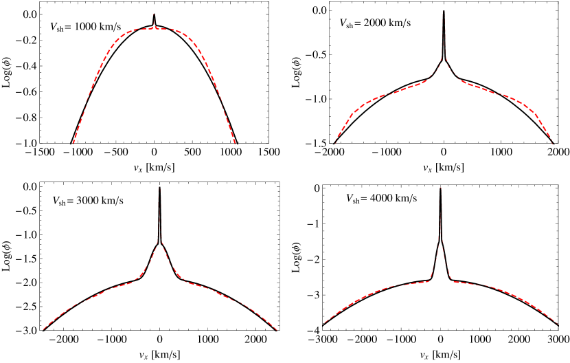
Figure 8.— Examples of fits with three Gaussian curves for different values of the shock velocity, in the NE case. The dotted lines represent the emission computed with our kinetic model, while the solid line is the best fit. The quality of the fit increases for larger values of $V_{sh}$. Notice that all profiles are normalized such that the peak value is equal to 1.

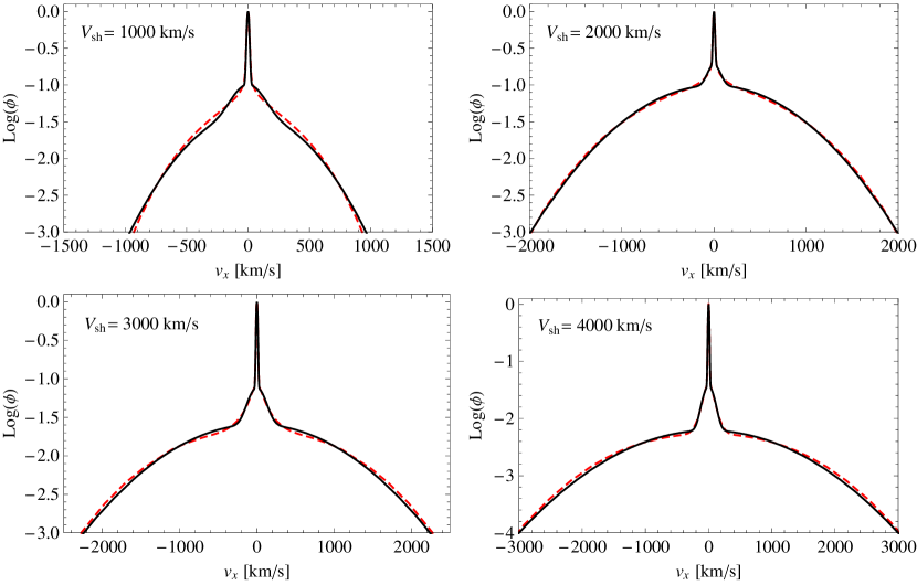
Figure 9.— The same as Fig. 8 but for the FE case.

Concerning the broad and the intermediate components, their FWHM are shown in the upper and lower panel of Fig. 10, respectively. As usual we plot the results for the NE and FE cases plus some intermediate cases for the electron-ion equilibration level. Our results for the FWHM of the broad component are in good agreement with previous calculations (e.g. Smith et al., 1991). The only exception concerns the NE case, which departs from the general trend for $V_{sh}<2500$ km/s. This behavior does not have a direct physical meaning and, as already noticed, is rather due to the particularly bad quality of the fit in this region of the parameter space. We remark that the quality of the fit rapidly improves for larger value of $\beta$ and the broad line width resulting from the fit becomes very close to the actual width when $\beta_{down}\buildrel>\over{{}_{\sim}}0.01$.

As first pointed out by Chevalier et al. (1980), the FWHM of the broad line is a direct measurement of the proton temperature downstream. As a consequence it only depends on the values of $V_{sh}$ and $\beta_{down}$. This result can be easily understood using a plane parallel shock model for a totally ionized plasma, which gives a proton temperature equal to $T_{i}=3m_{p}V_{sh}^{2}/16(1+\beta_{down})k_{B}$, where $m_{p}$ is the proton mass and $k_{B}$ the Boltzmann constant. As we showed in Paper I, this result still remains a good approximation when the plasma is only partially ionized and the neutral return flux is taken into account. On the other hand, a deviation of the proton temperature from this estimate can be induced by the presence of helium. In fact, immediately downstream of the shock, helium nuclei thermalize at a temperature $m_{He}/m_{p}$ times larger than the protons’ one. If helium and protons thermalize at the same temperature on a length scale smaller than the excitation length scale, the mean temperature of hot hydrogen produced by CE with hot protons is larger than the prediction without helium. As a consequence the FWHM is expected to be larger. Indeed, the presence of helium was taken into account by van Adelsberg et al. (2008), which found for the broad component a FWHM about 15-18% larger than the one found in our calculations.

Let us now consider the width of the intermediate component (lower panel of Fig. 10). In this case, for $1000<V_{sh}<5000$ km/s, the FWHM ranges between 100 and 300 km/s. A peak is present for $2000<V_{sh}<3500$ km/s, depending on the level of electron-ion equilibration. Once again, we notice that for $V_{sh}<1500$ km/s the FWHM obtained from the fit procedure is not well determined in that the intermediate component departs from a pure Gaussian shape. Moreover, the emission due to the broad component becomes much larger than the contribution of the intermediate one, which, in turn, becomes less distinguishable.

Observational evidences, compatible to what we call here intermediate component, have been reported in several works, even if such evidences have never been related to the neutral-induced precursor. The most interesting case is the H$\alpha$ line profile detected from the “Knot g” of the Tycho’s SNR by Ghavamian et al. (2000). There, an observation of H$\alpha$ emission performed with high spectral resolution suggests the presence of two superimposed lines: a narrow one, with a FWHM of $\sim 44$ km/s, plus a second, less pronounced line, whose FWHM is $\sim 150$ km/s. Such a width is fully compatible with the FWHM of the intermediate component resulting from our calculations. On the other hand it is important to stress that the Knot g is a complex region where density variations of the ISM produce a non-spherical shock, hence the observed line profile could also result from projection effects. For this reason observations with better spatial and spectral resolution are required in order to disentangle geometrical effects from physical effects. The Balmer emission detected from Tycho is not an isolated case. Several spectra observed from Balmer-dominated shocks show evidence of narrow H$\alpha$ lines with non-Gaussian “wings” (see e.g. Smith et al., 1994). We suggest that such wings could be the signature of the intermediate component.

In spite of this interesting connection, in the present work we avoid performing a detailed comparison between theoretical predictions and observations. The reason is that although the calculations presented here represent a considerable step forward in the description of collisionless shocks in partially ionized media, they still remain incomplete. Aside from some minor complications that need to be taken into account (like the presence of helium or projection effects arising from deviations from plane geometry), a major role in determining the shape of the H$\alpha$ line is played by the presence of CRs, which are not yet included here. In fact, it is widely accepted that efficient CR acceleration changes the global shock structure, generating an upstream precursor that is, to some extent, similar to the neutral-induced precursor but develops on a different length scale. Effects induced by CRs could be especially relevant for the Tycho’s SNR, which has been suggested to accelerate CRs efficiently Morlino & Caprioli (2012). In passing we notice that the efficient acceleration of CRs is the most plausible explanation of the relatively wide narrow Balmer line found in Tycho (FWHM of $\sim 44$ km/s).

It is worth noticing that alternative explanations for the non-Gaussian wings have also been proposed. For example, Raymond et al. (2008) suggest that deviations from the Gaussian profile could be the result of a non-Maxwellian proton distribution downstream. In fact, neutral atoms that become ionized could settle into a bi-spherical distribution (similar to that of pickup ions in the solar wind) that would then introduce a non-Gaussian contribution to the line core. We recall that in the present work, as well as in Paper I, we do not include such an effect, but we assume that, soon after being ionized, atoms thermalize with the rest of ions.

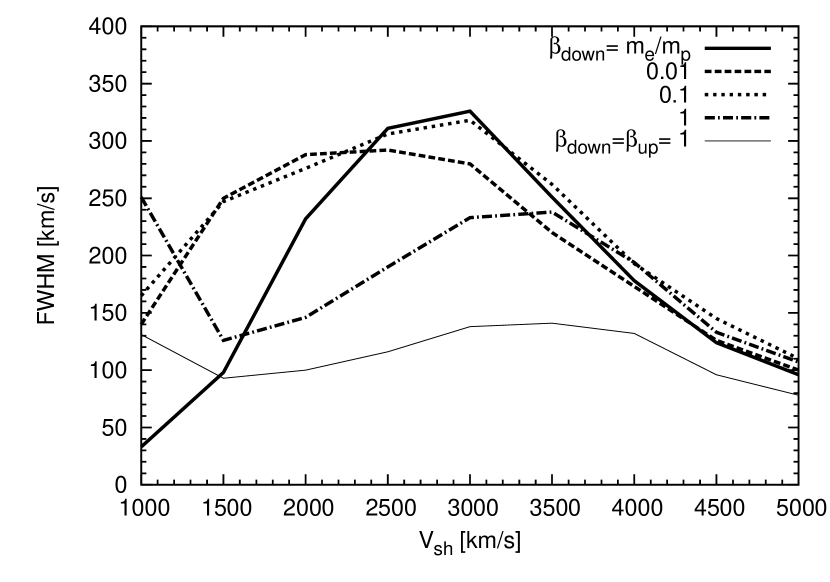
Figure 10.— FWHM for broad (upper panel) and intermediate components (lower panel) resulting from the the fit of total H$\alpha$ emission with 3-Gaussian distributions.

4.3. H$\alpha$ emission from the upstream

This section is devoted to highlight some features of the H$\alpha$ emission from the upstream region. This is a crucial observable in order to understand the effects produced by CR acceleration, as we will show in a forthcoming paper. In the near future, observations could reach good enough spatial and spectral resolution so as to provide detailed spectra at different distances from the shock position, which makes the exercise of analyzing the details of the emission from the upstream especially interesting.

As we already showed in Fig. 2 the upstream region could radiate up to 40% of the total Balmer emission in the case of full electron-ion temperature equilibration. On the other hand if $\beta_{up}\buildrel<\over{{}_{\sim}}0.01$ the upstream emission drops below 1% of the total. The line profile in the upstream emission is quite different from the one produced in the downstream region. In fact only the narrow and the intermediate lines are present. This is clearly shown in Fig. 11 where the upstream line profile at different distances from the shock is shown for the cases of FE and partial equilibration and for $V_{sh}=2000$ and 4000 km/s. We chose the following distances: $z=1\times,2\times$ and $5\times L_{\rm mfp}$, where $L_{\rm mfp}=1/(\sigma_{ce}n_{\rm tot})\sim 10^{16}$ cm, and the charge-exchange cross section is approximated as $\sigma_{ce}\sim 10^{-15}$ cm². As we move far away from the shock, the FWHM of the intermediate line decreases as a consequence of a reduction of the temperature in the precursor, while the narrow line has always the same FWHM. The total emission falls down at a distance of $\sim$few $L_{\rm mfp}$. This distance corresponds to the position where the electron temperature falls below the threshold of $\approx 1.5\times 10^{5}$K discussed in the second paragraph of § 4.1. This point moves further from the shock for larger values of $\beta_{up}$ as can be clearly seen in Fig. 12, where we plot the integrated line emission as a function of the position only in the upstream, distinguishing the contribution of the narrow and intermediate line and for different values of the shock velocity. When we have FE the contribution of the intermediate line is always smaller than that of the narrow line, but for lower equilibration levels the ratio of intermediate over narrow emission increases and for $\beta_{up}=0.1$ the two lines contribute at roughly the same level. These findings are summarized in Fig. 13.

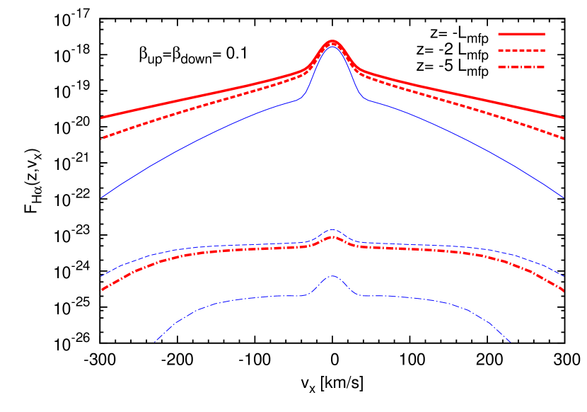
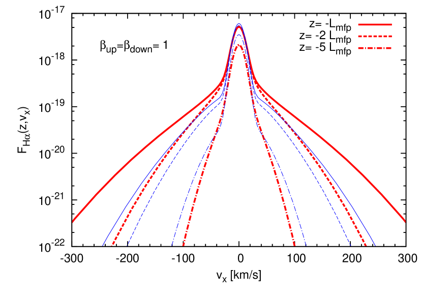
Figure 11.— Emissivity profile at three different locations in the upstream for partial equilibration, $\beta_{up}=\beta_{down}=0.1$ (upper panel), and FE, $\beta_{up}=\beta_{down}=1$ (lower panel). Thick (red) lines show the case for $V_{sh}=2000$ km/s while thin (blue) lines are for $V_{sh}=4000$ km/s.

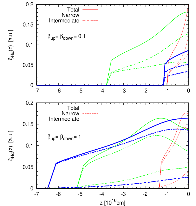
Figure 12.— Spatial emissivity profile of the H$\alpha$ line in the upstream. The upper panel shows the case of partial electron-ion equilibration with $\beta_{up}=\beta_{down}=0.1$ while the lower panel shows the FE case. Dashed and dot-dashed lines show the contribution of narrow and intermediate lines, respectively, while the solid line is the total emission. The line thickness (and color) distinguishes the different shock velocities: 1000 (thin-red), 2000 (middle-green) and 4000 km/s (thick-blue).

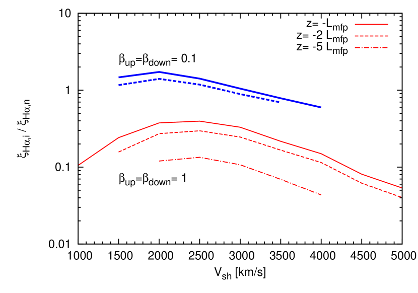
Figure 13.— Ratio of the intermediate to narrow H$\alpha$ emission at different locations in the upstream, as a function of the shock velocity. Different line shapes correspond to different locations, as indicated in the label. Thick (blue) lines show the partial equilibration case, while thin (red) lines show the FE case. The region of the parameter space where the H$\alpha$ emission drops at a level of $10^{-4}$ times the peak value are not shown in the plot. For example, for the case of partial equilibration at a distance of $5L_{\rm mfp}$ the emission is always below this threshold.

4.4. Simulated observations

Although the three-Gaussian fit presented in Section § 4.2 catches the essence of the expected distorsions in the Balmer lines, it does not reflect the whole complexity involved in fitting observed H$\alpha$ line profiles. Actual data are affected by a number of instrumental and statistical issues, the most obvious of which (and the only ones that we will investigate here) are: the limited spectral resolution of the instrument, the Poisson noise of the line photons themselves, and any additional photon noise, either due to the astronomical or to the instrumental background.

For the simulations presented here we have used the line profile computed for $V_{sh}=3000$ km/s (and with an ion fraction of 50%), $\beta_{down}=m_{e}/m_{p}$, $T_{e}$(up)$=10^{4}$ K. This situation is the one plotted as a dotted line in the upper panel of Fig. 4.

As for the observational parameters, we will adopt a published observation of an H$\alpha$ line profile in SN 1006 Ghavamian et al. (2002) as the reference for the instrumental parameters as well as for the flux levels. In that observation, the instrumental resolution is $4.5$ Å, corresponding to 205 km/s, while the dispersion per pixel is 0.27 times the resolution; the total number of photons measured in the line is about $10^{9}$ (for a 140 min integration time, with a 4-m class telescope), while the background noise level is about 3000 photons/Å: these photon numbers are for the whole spectrograph slit and integration time, as specified by Ghavamian et al. (2002).

Fig. 14 shows the results of a 2-Gaussian fit to simulated data, obtained combining the model with the instrumental parameters mentioned above. As shown by the residuals, in this case the quality of the observation is not sufficient to investigate details, beyond the mere separation of a narrow and a broad component.

Figure 14.— Results of a 2-Gaussians fit to a simulated line profile, obtained by downgrading our Model with a typical instrumental resolution and photon noise, and adding Poisson noise (see text for details). The upper panel shows the simulated data (solid line), together with the best-fit narrow line (dashed line) and broad line (dotted line) components; while the lower panel shows the residuals after subtraction of the best-fit solution.

We have then explored several combinations of the observational parameters, focusing on the spectral resolution (expressed in terms of velocity resolution, $v_{res}$) and on the photon statistics (expressed in terms of the total number of photons in the line, $N_{phot}$). As for the instrumental dispersion per pixel, we have kept the ratio of 0.27 times the resolution, as in Ghavamian et al. (2002), while we have usually adopted the background noise level given above. We have also tried with a much lower background noise level, but, of course, even in this case, the noise component associated with the photons of the line itself cannot be eliminated.

We have used a grid of simulations to investigate, on the $\log(N_{phot})$–$v_{res}$ parameter plane, the behavior of 2-Gaussian and 3-Gaussian fits. In both cases we have chosen a grid of $25\times 25$ points, suitably positioned in the parameter plane. In order to minimize the “noisy” look in the figure (a natural consequence of the fact that each simulation includes random noise), we have performed a large number (100) of simulations for each point; out of them, we have discarded the 5 cases with the highest $\chi^{2}$ value as well as the 5 ones with the lowest $\chi^{2}$ value, and we have then taken the average $\chi^{2}$ of the remaining ones. The results are shown in Fig. 15.

Figure 15.— Behaviour of the 2-Gaussians (upper panel) and 3-Gaussians (lower panel) fits on simulated data obtained starting from our Model. We have investigated the parameter plane $\log_{10}(N_{phot})$–$v_{res}$. The three contours in each panel, drawn respectively as a solid, a dashed and a dotted line, indicate the 1-$\sigma$, 2-$\sigma$ and 3-$\sigma$ confidence level. The contours are obtained by interpolating over a $40\times 40$ data grid, each point of which is an average value of 50 independent simulations. These plots show that only on the lower right side of the panels the quality of the observations is good enough to allow outlining deviations from, respectively, a 2- or 3-Gaussians profile.

As a result, for our Model, we may see that, for a line photon statistics of about $10^{9}$ photons, a spectral resolution better than about 180 km/s is required to show (at a 3-$\sigma$ confidence level) that a 2-Gaussian fit is not adequate; while a resolution better than about 70 km/s is required to challenge the 3-Gaussian fit. Even if having more photons does matter, in general the photon statistics does not seem to be a parameter as crucial as the spectral resolution. Of course, in order to resolve the narrowest spectral component a considerably higher resolution is required; otherwise, it will be detected only as an “unresolved spectral component”.

4.5. Line intensity ratios

Another observable that may be useful in order to constrain shock parameters is the ratio between the intensities of broad and narrow components, $I_{b}/I_{n}$. This information is usually used in combination with the FWHM of the broad component, in order to infer simultaneously both $V_{sh}$ and the level of electron-ion equilibration downstream Heng (2009). The presence of the neutral-induced precursor complicates a bit this exercise because the upstream equilibration also plays a role, as we show below.

At this point we need to comment on an observational caveat. When Balmer emission is observed with a high spectral resolution, in order to resolve the narrow component, usually the broad component is not detected due to the high spectral dispersion (se e.g. Ghavamian et al., 2000). In order to measure the intensity of the broad component, which allows one to estimate the $I_{b}/I_{n}$ intensity ratio, observations must be performed instead with a lower spectral resolution, typically equivalent to a velocity resolution $\Delta v\sim 100-300$ km/s; but this does not allow to resolve simultaneously all three components, because at such resolution the intermediate component cannot be distinguished from the narrow one, as they appear as a single line. As a consequence, in order to provide an estimate of $I_{b}/I_{n}$, we first convolve the line profile obtained by our kinetic calculation, with the typical instrumental resolution, $\Delta v$. Then we fit the convolved emission with a two-Gaussian profile, evaluating both $I_{b}$ and $I_{n}$ from the fitting curves. We choose $\Delta v=150$ km/s, which corresponds to a wavelength resolution of $\Delta\lambda=3.3$ Å.

The results are shown in Fig. 16, where different lines represent different assumptions for the electron-ion equilibration level. The qualitative behaviour is similar to what predicted by previous studies Smith et al. (1991); Heng & McCray (2007), even if some differences can be noted. Our results are, in general, a factor 2–3 larger than what predicted by Smith et al. (1991) (see their Fig. 8). Their equilibrated case (which corresponds to our dot-dashed line) peaks at $V_{sh}=2000$ km/s and is $I_{b}/I_{n}\simeq 2$ while our curve peaks at $V_{sh}\simeq 1500$ km/s with $I_{b}/I_{n}\simeq 5$. In fact, it is rather difficult to perform a close comparison between the ratios computed by different authors, because of substantial differences in the model assumptions, in the methods used, in the assumed chemical composition, and even in the cross sections adopted for the various processes: therefore we take the above level of differences as acceptable.

From the observational point of view, in all the SNRs for which $I_{b}/I_{n}$ has been measured, an intensity ratio above 1.2 has never been seen, while in most cases it falls below unity (see e.g. Heng & McCray, 2007). If we assume no equilibration upstream, this result suggests an intermediate value for the electron-ion equilibration efficiency downstream. On the other hand we also see that the FE model (both upstream and downstream) predicts an intensity ratio $<1$ for all shock velocities considered. Unfortunately, for given values of $I_{b}/I_{n}$ and $V_{sh}$ there is a degeneracy for the values of $\beta_{up}$ and $\beta_{down}$.

Moreover, the trend of $I_{b}/I_{n}$ with respect to the electron-ion equilibration is not monotonic. As first noticed by Smith et al. (1991), NE and FE cases do not represent the extreme values of the intensity ratio. We see, in fact, that for intermediate values of $\beta_{down}$, $I_{b}/I_{n}$ drops below the equilibrated case $\beta_{down}=1$.

Figure 16.— Ratio of the broad to narrow H$\alpha$ emission versus shock velocity after the convolution with experimental velocity resolution of $\Delta v=150$ km/s. Different lines represent different cases of electron-ion equilibration efficiency. Thick curves all assume non-equilibrium upstream, while the thin curve shows the FE case.

5. Conclusions

In this paper we computed the H$\alpha$ emission produced by a collisionless shock that propagates into a partially ionized medium. In order to do this, we first derived the evolution of the various species across the shock, by using the kinetic model developed in Paper I. This model applies to plane-parallel non-radiative shocks in the steady state where ions are treated as a fluid, while neutral particles are described using the full 3D velocity distribution function. On top of this solution we then computed the Balmer emission produced by collisional excitation of hydrogen atoms with both ions and electrons, as well as by CE events leading to neutrals in excited states. Results for the spatial emission and for the line profile of H$\alpha$ are presented for a shock seen edge-wise, varying the shock speed, the initial ionization fraction and the electron-ion equilibration level.

According to the traditional picture Chevalier & Raymond (1978), the H$\alpha$ profile detected from Balmer dominated shocks usually consists of two components: a narrow one, whose width reflects the temperature of the upstream medium, and a broad one, due to neutrals that have undergone CE with hot protons in the downstream region.

This picture is however an oversimplification of what happens in reality, mainly for two reasons: i) it assumes that neutrals can be described as a fluid, namely with Maxwellian velocity distributions; ii) it does not take into account the effect induced by the neutral precursor. In fact, the latter point is a natural consequence of the former one: already in Paper I we showed that, for a wide range of shock velocities, a fraction of the hot neutrals produced downstream can recross the shock toward upstream, giving rise to a neutral return flux, and that the interaction of these neutrals with the upstream ions produces a precursor region where the incoming plasma is heated and slowed down. In this paper we have shown that the neutral-induced precursor is responsible for the production of a new H$\alpha$ line component, whose width is intermediate between the narrow and the broad lines, being around few hundreds km/s for a shock speed of a few thousands km/s. This intermediate line is due to cold hydrogen atoms that have undergone CE with warm protons in the neutral-induced precursor, hence its width reflects the mean temperature of the precursor. In addition, we found that the profiles of the intermediate and broad-line components may deviate from pure Gaussians, and that these deviations could be detected by carrying out observations of suitably high quality.

A natural question to ask is whether the heating produced in the neutral precursor could explain the anomalous width of narrow lines, which has already been observed in some Balmer filaments associated with several SNR shocks Smith et al. (1994); Hester et al. (1994). Our results show that this is not the case: the bulk of incoming neutrals does not interact with ions in the neutral precursor, because its extent, which corresponds to the interaction length of the returning neutrals, is much smaller than the CE length of the incoming neutrals. Instead, as we already discussed, the fraction of incoming neutrals interacting with ions in the precursor will give rise to the intermediate H$\alpha$ line. Therefore, we conclude that other mechanisms, like for instance a CR-induced precursor, should be invoked to explain an anomalous width of the narrow-line component.

Remarkably, some observations point towards the existence of intermediate lines compatible with our predictions: narrow lines detected from Tycho and from other SNRs show non-Gaussian wings which could be explained with the existence of a third line component. At the moment this result must be taken with care because projection effects could also be responsible for the observed line profiles. Better spatial and spectral resolution are needed to disentangle these effects. Unfortunately, the majority of these observations do not have the spectral resolution required to carry out a satisfactory 3-component fit. In order to estimate the experimental requirements necessary to identify the intermediate line, we compared our theoretical H$\alpha$ profile with simulated observations, which take into account both instrumental resolution and Poisson noise of the line photons. As a result, for a typical line photon statistics of about $10^{9}$ photons, a spectral resolution better than $\sim 70$ km/s is required to separately identify all three components.

The presence of the intermediate line component may also affect the evaluation of the broad to narrow line intensity ratio, $I_{b}/I_{n}$. This quantity is usually used together with the broad line width, in order to estimate the level of electron-ion temperature equilibration in the post-shock region. Evaluation of $I_{b}/I_{n}$ is usually done from observations with resolution $>100$ km/s, necessary to detect both the narrow and the broad lines.

This implies that the intermediate line is not resolved and that its emission contributes to the observed narrow line intensity. We have included this effect in the evaluation of $I_{b}/I_{n}$, and have shown how this ratio changes varying the electron-ion equilibration downstream. As already pointed out by several authors, if efficient electron-ion equilibration occurs downstream, the width of the broad line is reduced because a fraction of the kinetic energy of incoming protons is transferred to electrons.

In addition to the effects produced by electron-ion equilibration downstream, we investigated what happens if equilibration also occurs in the precursor region. Interestingly, we showed that, increasing the efficiency of equilibration beyond a few percent, electrons can collisionally excite hydrogen atoms, giving rise to Balmer emission also from the precursor region. For $V_{sh}\approx$ 2500 km/s, if equilibration is complete ($T_{e}=T_{p}$), the emission from the precursor can contribute up to $\sim 40\%$ of the total H$\alpha$ emission. This result can be instrumental to explain the results recently published by Lee et al. (2010). They observe the Eastern limb of Tycho’s SNR, finding a gradual increase of H$\alpha$ intensity just ahead of the shock front, which they interpret as emission from a thin shock precursor. They estimate that the precursor emission may contribute up to 30%-40% of the total narrow component emission and suggest that the precursor is likely due to CRs. In light of our results it is clear that a correct interpretation of the pre-shock H$\alpha$ emission requires also the evaluation of the emission produced by the neutral induced precursor.

In a forthcoming paper, currently in preparation, we will describe the theory of collisionless shocks in partially ionized media in the presence of accelerated particles that exert a pressure on the incoming ions. In other words, we will generalize the non-linear theory of particle acceleration in collisionless shocks to include the neutral return flux discussed in Paper I. In the same paper we will calculate the shape of the Balmer lines as they are affected by accelerated particles, and show how to use the widths of the narrow, intermediate and broad components of the Balmer line as tools to measure the CR acceleration efficiency in SNRs.

Aknowledgments

We thanks an anonymous referee for his/her valuable suggestions which allowed us to improve the quality of the present work. We are very grateful to Kevin Heng for providing some of the cross sections used in this work. Our work is partially funded through grants PRIN-INAF 2010 and ASTRI.

References

- van Adelsberg et al. (2008) van Adelsberg, M., Heng, K., McCray, R., & Raymond, J.C. 2008, ApJ, 689, 1089
- Balança et al. (1998) Balança, C., Lin, C. D & Feautier, N., 1998, J Phys. B, 31, 2321
- Barnett el al. (1990) Barnett, C. F., Hunter, H. T., Fitzpatrick, M. I., Alvarez, I., Cisneros, C., & Phaneuf, R. A. 1990, Collisions of H, H2, He and Li Atoms and Ions with Atoms and Molecules (Rep. ORNL-6086/V1; Oak Ridge: Oak Ridge Natl. Lab.)
- Bray & Stelbovics (1995) Bray, I., & Stelbovics, A. T. 1995, AAMP 35, 209
- Belkić et al. (1992) Belkić, D., Gayet, R. & Salin, A., 1992, At. Data Nucl. Dtata Tables, 51, 59
- Blasi et al. (2012) Blasi, P., Morlino, G., Bandiera, R., Amato, E., Caprioli, D., 2012, ApJ, 755, 121
- Chevalier et al. (1980) Chevalier, R. A., Kirshner, R. P., and Raymond, J. C., 1980, ApJ, 235, 186
- Chevalier & Raymond (1978) Chevalier, R. A., Raymond, J. C. 1978, ApJ, 225, L27
- Ghavamian et al. (2007) Ghavamian, P., Laming, J. M., Rakowski, C. E. 2007, ApJ, 654, L69
- Ghavamian et al. (2000) Ghavamian, P., Raymond, J., Hartigan, P. and Blair, W. B. 2000, ApJ, 535, 266
- Ghavamian et al. (2001) Ghavamian, P., Raymond, J. C., Smith, R. C., & Hartigan, P. 2001, ApJ, 547, 2005
- Ghavamian et al. (2002) Ghavamian, P., Winkler, P. F., Raymond, J. C., Long, K. S. 2002, ApJ, 572, 888
- Harel et al. (1998) Harel, C., Jouin, H. & Pons, B., 1998, At. Data Nucl. Dtata Tables, 68, 279
- Helder et al. (2009) Helder, E. et al. 2009, Science, 325, 719
- Heng (2009) Heng, K. 2009, PASA, 27, 23
- Heng & McCray (2007) Heng, K., McCray, R. 2007, MNRAS, 654, 923
- Heng & Sunyaev (2008) Heng, K., Sunyaev, R. A. 2008, A&A, 481, 117
- Hester et al. (1994) Hester, J. J., Raymond, J. C. & Blair, W. P. 1994, ApJ 420, 721
- Janev & Smith (1993) Janev, R. K., & Smith, J. J. 1993, Cross Sections for Collision Processes of Hydrogen Atoms with Electrons, Protons and Multiply Charged Ions (Vienna: Int. At. Energy Agency)
- Lee et al. (2010) Lee, J. J., Raymond, J. C., Park, S., Blair, W. P., Ghavamian, P., Winkler, P. F., & Korreck, K. 2010, ApJ, 715, L146
- Lim & Raga (1996) Lim, A. J. & Raga, A. C. 1996, MNRAS, 280, 103
- Morlino & Caprioli (2012) Morlino, G. & Caprioli, D. 2012, A&A, 538, 81
- Raymond et al. (2008) Raymond, J. C., Isenberg, P. A. & Laming, J. M. 2008, ApJ, 682, 408
- Rakowsky (2005) Rakowsky, C. E. 2005, AdSpR, 35, 1017
- Smith et al. (1994) Smith, R. C., Raymond, J. C., & Laming, J. M. 1994, ApJ, 420, 286
- Smith et al. (1991) Smith, R. C., Kirshner, R. P., Blair, W. P. & Winkler, P. F. 1991, ApJ, 375, 652
- Sollerman et al. (2003) Sollerman, J., Ghavamian, P., Lundqvist, P. & Smith, R. C. 2003, A&A, 407, 249
- Tseliakhovich et al. (2012) Tseliakhovich, D., Hirata, C. M.; Heng, K. 2012, MNRAS, 422, 2357