Green’s function for symmetric loading of an elastic sphere with application to contact problems

Abstract.

A compact form for the static Green’s function for symmetric loading of an elastic sphere is derived. The expression captures the singularity in closed form using standard functions and quickly convergent series. Applications to problems involving contact between elastic spheres are discussed. An exact solution for a point load on a sphere is presented and subsequently generalized for distributed loads. Examples for constant and Hertzian-type distributed loads are provided, where the latter is also compared to the Hertz contact theory for identical spheres. The results show that the form of the loading assumed in Hertz contact theory is valid for contact angles up to about 10 degrees. For larger angles, the actual displacement is smaller and the contact surface is no longer flat.

1. Introduction

Contact between spheres has intrigued researchers for more than a century, and still no simple closed-form analytical solution exists. One of the first and most important developments in the field, due to Heinrich Hertz [1] in 1881, is an approximate solution for the normal, frictionless contact of linear elastic spheres. The major assumption in Hertz’s model is that the contact area was small compared to the radii of curvature, which has served as a useful engineering approximation in many applications. Ever since then many have tried to relax this assumption while maintaining a compact, workable solution. The Green’s function for symmetric loading on a sphere provides the means to find the exact response for arbitrary loading, a first step towards improving on Hertz’ classic solution. Existing forms of the Green’s function are however not suitable for fast and ready computation, either due to slow convergence of series or analytically cumbersome expressions. The goal of the present paper is to provide an alternative form of the Green’s function suitable for fast computation of solutions under arbitrary loading.

Sternberg and Rosenthal [2] present an in-depth study of the nature of the singularities on elastic sphere loaded by two opposing concentrated point forces. As expected, the dominant inverse square singularity in the stress components can be removed by subtraction of an appropriate multiple of Boussinesq’s solution for a point load at the surface of a half space. Sternberg and Rosenthal showed that the quickly convergent residual field retains a weaker singularity of logarithmic form, a result that is also evident in the solution developed here. The singular solutions obtained by Sternberg and Rosenthal were extended to arbitrarily oriented point forces by Guerrero et al. [3]. Our interest here is in developing an analogous separation of the Green’s function (circular ring loading). In this regard, a relatively compact form of the Green’s function for the sphere was derived by Bondareva [4] who used it to solve the problem of the weighted sphere. In [5], Bondareva formulates an example with a sphere contacting a rigid surface. This has been used to solve the rebound of a sphere from a surface [6]. Bondareva’s solution starts with the known series expansion [7] for the solution of the elasticity problem of a sphere, and replaces it with finite integrals of known functions.

In this paper we introduce an alternative form for the Green’s function for a sphere, comprised of analytical functions and a quickly convergent series. No direct integration is required. The methodology for determining the analytical functions is motivated by the simple example of a point load on a sphere, for which we derive a solution similar in spirit to that of [2], but using a fundamentally different approach: partial summation of infinite series as compared with a functional ansatz. The present methods allows us to readily generalize the point load solution to arbitrary symmetric normal loading. A typical contact problem involves solving a complicated integral equation for the contact stress once a displacement is specified. Instead, we will use the derived Green’s function in the direct sense, solving for the displacements for a given load. This is used to check the validity of Hertz contact theory through the assumed form of the stress distribution.

The outline of the paper is as follows. The known series solution for symmetric loading on a sphere is reviewed in §2. The proposed method for simplification is first illustrated in §3 by deriving a quickly convergent form of the solution for a point force. The Green’s function for symmetric loading is then developed in §4, and is illustrated by application to different loadings. Conclusions are given in §5.

2. Series solution

Consider a solid sphere of radius $R$, with surface $r=R$, $0\leq\theta\leq\pi$, in spherical polar coordinates ($r$, $\theta$, $\phi$). The sphere is linear elastic with shear modulus $G$ and Poisson’s ratio $\nu$. The surface is subject to tractions

$$\sigma_{r\theta}=0,\ \ \sigma_{r\phi}=0,\ \ \sigma_{rr}=\sigma(\theta),\ \ \text{for }\ r=R,\ 0\leq\theta\leq\pi,\ 0\leq\phi<2\pi.$$ (1)

Using the known properties of Legendre functions, see. eqs. (45), allows us to express the normal stress as

$$\sigma(\theta)=\frac{1}{2}\sum\limits_{n=0}^{\infty}(2n+1)\sigma_{n}P_{n}(\cos\theta),$$ (2)

where the Legendre series coefficients are

$$\sigma_{n}=\int\limits_{0}^{\pi}\sigma(\phi)P_{n}(\cos\phi)\,\sin\phi\,d\phi.$$ (3)

The displacements and tractions for the sphere can also be represented in series form [8, eq. 5]

$$2Gu_{r} =\sum\limits_{n=0}^{\infty}\big{[}(n-2+4\nu)A_{n}r+B_{n}r^{-1}\big{]}\,r^{n}\,P_{n}(\cos\theta),$$ (4)

$$2Gu_{\theta} =\sum\limits_{n=1}^{\infty}\big{[}n(n+5-4\nu)A_{n}r+(n+1)B_{n}r^{-1}\big{]}\,r^{n}\,\frac{P_{n}^{1}(\cos\theta)}{n(n+1)},$$

$$\sigma_{rr} =\sum\limits_{n=0}^{\infty}\big{[}[n(n-1)-2(1+\nu)]A_{n}+(n-1)B_{n}r^{-2}\big{]}\,r^{n}\,P_{n}(\cos\theta),$$

$$\sigma_{r\theta} =\sum\limits_{n=1}^{\infty}\big{[}n[(n-1)(n+3)+2(1+\nu)]A_{n}+(n^{2}-1)B_{n}r^{-2}\big{]}\,r^{n}\,\frac{P_{n}^{1}(\cos\theta)}{n(n+1)},$$

with $B_{0}\equiv 0$, and $B_{1}$ corresponds to a rigid body translation via $2G{\bf u}(0,\cdot)=B_{1}{\bf e}_{z}$. It follows from (1) that

$$A_{0}=\frac{-\sigma_{0}}{2(1+\nu)},\ \ A_{1}=0,$$ (5)

$$A_{n}=-\frac{\sigma_{n}}{4R^{n}}\,\frac{(n+1)(2n+1)}{[n(n-1)+(2n+1)(1+\nu)]},\ \ n\geq 2,$$

$$B_{n}=\frac{-n}{n^{2}-1}\,[(n-1)(n+3)+2(1+\nu)]\,R^{2}A_{n},\ \ n\geq 2.$$

Thus, noting that $P_{n}^{1}(\cos\theta)=\frac{d}{d\theta}P_{n}(\cos\theta)$, we have

$$\begin{split}u_{r}(R,\theta)&=\frac{R}{4G}\,\Big{(}\frac{2(1-2\nu)}{1+\nu}\sigma_{0}+\sum\limits_{n=2}^{\infty}\sigma_{n}\bigg{(}\frac{2n+1}{n-1}\bigg{)}\bigg{(}\frac{2(1-\nu)n^{2}+\nu n-1+2\nu}{n^{2}+(1+2\nu)n+1+\nu}\bigg{)}\,P_{n}(\cos\theta)\Big{)},\\ u_{\theta}(R,\theta)&=\frac{R}{4G}\,\frac{d}{d\theta}\sum\limits_{n=2}^{\infty}\sigma_{n}\bigg{(}\frac{2n+1}{n-1}\bigg{)}\bigg{(}\frac{(-1+2\nu)n+2-\nu}{n^{2}+(1+2\nu)n+1+\nu}\bigg{)}\,P_{n}(\cos\theta).\end{split}$$ (6a)

Bondareva [4], using a different representation, replaced the infinite summation of Legendre functions by a combination of closed form expressions and an integral, each dependent on $\nu$. The integral term contains a logarithmic singularity which, together with the complex-valued nature of its coefficients, makes its evaluation indirect. Here we propose an alternative form for the Green’s function in a combination of closed-form expressions and a standard summation of Legendre functions that is, by design, quickly convergent.

3. Point force

3.1. Exact solution.

In order to illustrate the method, we first consider the simpler problem of the point force of magnitude $F$ applied at $\theta=0$ defined by

$$\sigma(\theta)=\frac{-F}{2\pi R^{2}}\,\lim_{\psi\downarrow 0}\,\frac{\delta(\theta-\psi)}{\sin\psi}\quad\Leftrightarrow\quad\sigma_{n}=\frac{-F}{2\pi R^{2}}$$ (7)

where we have used the property $P_{n}(1)=1$. The difficulty with the infinite summations (6) is two fold: first, it is not a suitable form to reproduce the singular nature of the Green’s function; secondly, it does not converge quickly as a function of the truncated value for $n$. The idea here is to replace the summation by closed form expressions plus a summation that is both regular and quickly convergent. The fundamental idea behind the present method is to write $u_{r}$, $u_{\theta}$ of eqs. (6) in the form

$$u_{r}(R,\theta) =\frac{-F}{8\pi GR}\bigg{(}4(1-\nu)S(\theta)+\sum\limits_{j=0}^{M}a_{j}(\nu)S_{j}(\theta)+f(\theta)\bigg{)},$$ (8a)

$$u_{\theta}(R,\theta) =\frac{-F}{8\pi GR}\frac{d}{d\theta}\bigg{(}\sum\limits_{j=0}^{M}b_{j}(\nu)S_{j}(\theta)+g(\theta)\bigg{)},$$ (8b)

where the functions $S(\theta)$ and $S_{j}(\theta)$ $(j=1,\ldots M)$, are closed-form expressions, in this case,

$$S(\theta) =\sum\limits_{n=0}^{\infty}P_{n}(\cos\theta)=\frac{1}{2}\csc\frac{\theta}{2},$$ (9a)

$$S_{j}(\theta) =\sum\limits_{n=0}^{\infty}\frac{P_{n+j}(\cos\theta)}{n+1},\ \ j=0,1,\ldots,$$ (9b)

and $f(\theta)$, $g(\theta)$ are regular functions of $\theta$ defined by quickly convergent series in $n$,

$$f(\theta)=\sum\limits_{n=0}^{\infty}C_{n}P_{n}(\cos\theta),\quad g(\theta)=\sum\limits_{n=0}^{\infty}D_{n}P_{n}(\cos\theta).$$ (10)

The coefficients $a_{0}$, $a_{1}$ $\ldots$ $a_{M}$ are defined so that $C_{n}=$O$(n^{-(M+2)})$ as $n\to\infty$. This criterion uniquely provides the constants $a_{0}$, $a_{1}$ $\ldots$ $a_{M}$ as solutions of a system of linear equations. Similarly, $b_{0}$, $b_{1}$ $\ldots$ $b_{M}$ are uniquely defined by $D_{n}=$O$(n^{-(M+2)})$ as $n\to\infty$.

Here we consider the specific case of $M=2$. Other values of $M$ could be treated in the same manner; however, we will show that $M=2$ is adequate for the purpose of improving convergence. In this case eq. (8) becomes

$$u_{r}(R,\theta)= \frac{-F}{8\pi GR}\,\Big{[}4(1-\nu)S(\theta)+a_{0}S_{0}(\theta)+a_{1}S_{1}(\theta)+a_{2}S_{2}(\theta)+f(\theta)\Big{]}$$

$$= \frac{-F}{8\pi GR}\,\Big{[}\sum\limits_{n=2}^{\infty}\Big{(}4(1-\nu)+\frac{a_{0}}{n+1}+\frac{a_{1}}{n}+\frac{a_{2}}{n-1}+C_{n}\Big{)}P_{n}(\theta)+C_{0}P_{0}(\theta)+C_{1}P_{1}(\theta)$$

$$+4(1-\nu)\Big{(}P_{0}(\theta)+P_{1}(\theta)\Big{)}+a_{0}\Big{(}P_{0}(\theta)+\frac{1}{2}P_{1}(\theta)\Big{)}+a_{1}P_{1}(\theta)\Big{]},$$ (11a)

$$u_{\theta}(R,\theta)= \frac{-F}{8\pi GR}\,\frac{d}{d\theta}\Big{[}b_{0}S_{0}(\theta)+b_{1}S_{1}(\theta)+b_{2}S_{2}(\theta)+g(\theta)\Big{]}$$

$$= \frac{-F}{8\pi GR}\,\frac{d}{d\theta}\Big{[}\sum\limits_{n=2}^{\infty}\Big{(}\frac{b_{0}}{n+1}+\frac{b_{1}}{n}+\frac{b_{2}}{n-1}+D_{n}\Big{)}P_{n}(\theta)$$

$$+b_{0}\Big{(}P_{0}(\theta)+\frac{1}{2}P_{1}(\theta)\Big{)}+b_{1}P_{1}(\theta)+D_{0}P_{0}(\theta)+D_{1}P_{1}(\theta)\Big{]},$$ (11b)

where the associated three functions $S_{j}(\theta)$, $j=0,1,2$ are (see the Appendix)

$$S_{0}(\theta) =\log\bigg{(}1+\csc\frac{\theta}{2}\bigg{)},$$ (12a)

$$S_{1}(\theta) =-S_{0}(\theta)-2\log\sin\frac{\theta}{2},$$ (12b)

$$S_{2}(\theta) =S_{1}(\theta)\cos\theta-2\sin\frac{\theta}{2}\bigg{(}1-\sin\frac{\theta}{2}\bigg{)}.$$ (12c)

Equations (8), (9a) and (12) indicate the expected Boussinesq-like $\theta^{-1}$ singularity as well as the weaker $\log\theta$ singularity first described by Sternberg and Rosenthal [2]. The logarithmic singularities in $S_{j}(\theta)$, $j=0,1,2$ can be compared to the potential functions $[D_{1}]$, $[D_{2}]$, and $[D_{3}]$ in equation (17) of [2], which provide a logarithmic singularity. In the present notation these are, respectively (using capital $\Phi$s so as not to be confused with the angle $\phi$, and making the substitution $\theta\rightarrow\pi-\theta$)

$$\Phi_{1}(\theta) =2\log\sin\frac{\theta}{2},\qquad\Phi_{2}(\theta)=-R\big{(}1+2\cos\theta\,\log\sin\frac{\theta}{2}\big{)},$$ (13a)

$$\Phi_{3}(\theta) =R^{2}\big{(}2(1-3\cos^{2}\theta)\log\sin\frac{\theta}{2}+\cos^{2}\theta-3\cos\theta-1\big{)}.$$ (13b)

These clearly display the same form of the singularity as in equations (12), but are otherwise different.

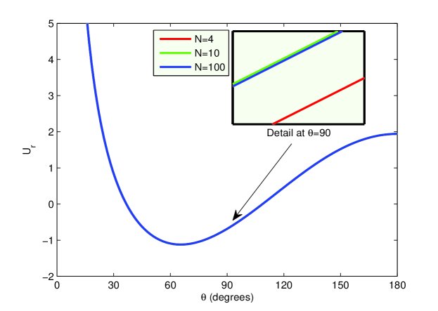
Figure 1. Convergence of the proposed expression for $U_{r}=\frac{-8\pi GR}{F}u_{r}$ in eq. (11). The magnified view at $\theta=\frac{\pi}{2}$ shows the difference in the value of $U_{r}$, which is $(U_{r})_{N=10}-(U_{r})_{N=4}=4.5259\cdot 10^{-4}$ and $(U_{r})_{N=100}-(U_{r})_{N=10}=-1.7059\cdot 10^{-5}$. The small plot is magnified by a factor of 11250.

Define the first two coefficients of $f(\theta)$ and $g(\theta)$ from (10) as

$$C_{0} =\frac{2(1-2\nu)}{1+\nu}-4(1-\nu)-a_{0},\quad C_{1}=-4(1-\nu)-\frac{1}{2}a_{0}-a_{1},$$ (14a)

$$D_{0} =-b_{0},\qquad\qquad\qquad\qquad\qquad D_{1}=-\frac{1}{2}b_{0}-b_{1}.$$ (14b)

The coefficients $a_{n}$ and $b_{n}$ are then found by comparing expression (11) to the series solution in (6), expanding both expressions for large $n$, and equating the coefficients of the same order terms. Thus, the original assumed form of the solution (8) implies

$$\sum\limits_{n=2}^{\infty}\frac{P_{n}(\theta)}{n^{2}+(1+2\nu)n+1+\nu}\Big{(}\frac{2n+1}{n-1}\Big{)}\times\begin{cases}\big{(}2(1-\nu)n^{2}+\nu n-1+2\nu\big{)}\\ \big{(}(-1+2\nu)n+2-\nu\big{)}\end{cases}$$ (15)

$$\qquad\qquad\qquad\qquad\qquad=\sum\limits_{n=2}^{\infty}P_{n}(\theta)\times\begin{cases}\big{(}4(1-\nu)+\frac{a_{0}}{n+1}+\frac{a_{1}}{n}+\frac{a_{2}}{n-1}+C_{n}\big{)},\\ \big{(}\frac{b_{0}}{n+1}+\frac{b_{1}}{n}+\frac{b_{2}}{n-1}+D_{n}\big{)},\end{cases}$$

where

$$\begin{split}a_{0}&=\frac{1}{2}(1+\nu)(1-2\nu)(-16\nu^{2}+8\nu+5),\\ a_{1}&=-32\nu^{4}+16\nu^{3}+30\nu^{2}-16\nu-1,\\ a_{2}&=16\nu^{4}-16\nu^{3}-5\nu^{2}+\frac{13}{2}\nu+\frac{1}{2},\\ b_{0}&=\frac{1}{2}(1+\nu)(16\nu^{2}-12\nu-1),\\ b_{1}&=-16\nu^{3}+4\nu^{2}+13\nu-4,\\ b_{2}&=8\nu^{3}-6\nu^{2}-\frac{5}{2}\nu+\frac{5}{2}.\end{split}$$ (16a)

The remaining coefficients $C_{n}$ and $D_{n}$ are then determined directly from (15)

$$C_{n} =\frac{(1+\nu)}{L_{n}}\Big{(}(6-a_{1}-6a_{2})n+a_{1}\Big{)}$$

$$=-\frac{(1+\nu)}{L_{n}}\Big{(}(64\nu^{4}-80\nu^{3}+23\nu-4)n+(32\nu^{4}-16\nu^{3}-30\nu^{2}+16\nu+1)\Big{)},$$ (17a)

$$D_{n} =\frac{(1+\nu)}{L_{n}}\Big{(}(6-b_{1}-6b_{2})n+b_{1}\Big{)}$$

$$=-\frac{(1+\nu)}{L_{n}}\Big{(}(32\nu^{3}-32\nu^{2}-2\nu+5)n+(16\nu^{3}-4\nu^{2}-13\nu+4)\big{)},$$ (17b)

where

$$L_{n}\equiv n(n^{2}-1)(n^{2}+(1+2\nu)n+1+\nu).$$ (18)

In summary, the new form of the point force solution is given by the displacements in eq. (11) where the functions and coefficients are given in eqs. (12)-(14), (16)-(18).

It is useful to note that the present approach, like that of Sternberg and Rosenthal [2], leads to a separation of the solution into a part that displays the singular behavior plus an additional part that is quickly convergent. Sternberg and Rosenthal’s solution was based on an ansatz [2, eq. (38) ] motivated by separation of the stress into a Boussinesq term with leading order singularity plus a residual field. Our approach is somewhat different, in that we regularize the infinite series solution directly by partial summation. The net effect is essentially the same as in [2, eq. (38) ] for the point load. However, the present method can be easily adapted to the more general case of the Green’s function for a circular (ring) load, see §4. The analogous generalization of Sternberg and Rosenthal’s method is not as obvious.

3.2. Numerical examples.

In the following examples we introduce the integer $N$ as the truncation value of the series in eqs. (10). The Poisson’s ratio was taken to be $0.4$. Displacements have been normalized by the constant coefficient of the series as $U_{i}={-8\pi GR}F^{-1}u_{i}$, where $i=r,\theta$. Figures 1 and 2 show the rate of convergence of the displacements given by eq. (11), whereas Figures 3 and 4 compare the displacements in eqs. (6) with eqs. (11).

By design, the proposed expression (eq. (11)) converges much faster than the existing expression (eq. (6)) as seen in Figures 3 and 4. Looking at the convergence of the proposed expressions with the truncation value $N$, Figures 1 and 2, we can suggest that the analytic portion of the expression alone gives close results. However, it should be noted that one cannot get rid of the first two terms in the series for $f(\theta)$ and $g(\theta)$ because of their large magnitudes. As far as the general behaviour of the normalized displacements with $\theta$, we see that they increase asymptotically approaching $\theta=0$, change sign between $36.7^{\circ}$ and $108.7^{\circ}$ for $U_{r}$ ($7.27^{\circ}$ and $80.83^{\circ}$ for $U_{\theta}$), and have a minimum at $65.5^{\circ}$ for $U_{r}$ ($24.6^{\circ}$ for $U_{\theta}$). This is difficult to see in the Figures, but due to symmetry of the loading, the displacement $U_{\theta}$ must have a value of zero at $\theta=0$.

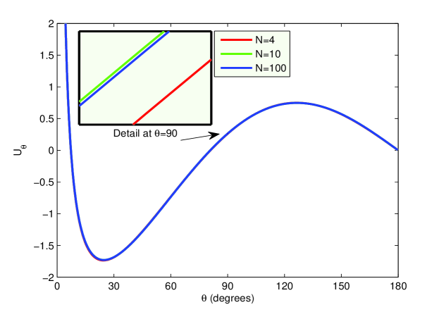
Figure 2. Convergence of $U_{\theta}=\frac{-8\pi GR}{F}u_{\theta}$ given in eq. (11). The magnified view at $\theta=\frac{\pi}{2}$ shows the difference in the value of $U_{\theta}$, which is $(U_{\theta})_{N=10}-(U_{\theta})_{N=4}=2.4097\cdot 10^{-3}$ and $(U_{\theta})_{N=100}-(U_{\theta})_{N=10}=-1.5040\cdot 10^{-4}$. The small plot is magnified by a factor of 1200.

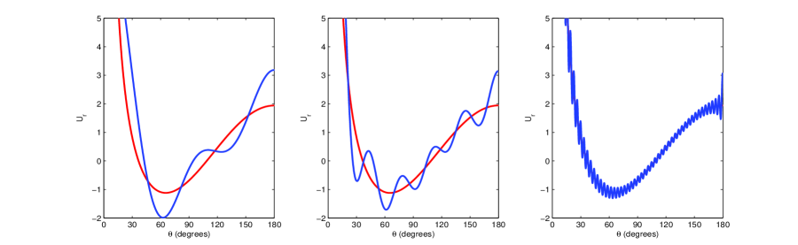
Figure 3. Comparison of the convergence of $U_{r}=\frac{-8\pi GR}{F}u_{r}$ with the truncation value $N$ for the existing expression (eq. (6), shown in blue) and the expression proposed herein (eq. (11), shown in red). Left to right: $N$=4, 10, 100.

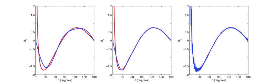
Figure 4. Comparison of the convergence of $U_{\theta}=\frac{-8\pi GR}{F}u_{\theta}$ with the truncation value $N$ for the existing expression (eq. (6), shown in blue) and the expression proposed herein (eq. (11), shown in red). Left to right: $N$=4, 10, 100.

4. Green’s function

4.1. A fast convergent form for the Green’s function

The surface displacements for arbitrary loading may be written, by analogy with the ansatz (8) for the point force, and generalizing the latter,

$$u_{r}(R,\theta) =\frac{R}{4G}\int_{0}^{\pi}\bigg{(}4(1-\nu)S(\theta,\phi)+\sum\limits_{j=0}^{M}a_{j}(\nu)S_{j}(\theta,\phi)+f(\theta,\phi)\bigg{)}\,\sigma(\phi)\sin\phi d\phi,$$ (19a)

$$u_{\theta}(R,\theta) =\frac{R}{4G}\frac{d}{d\theta}\int_{0}^{\pi}\bigg{(}\sum\limits_{j=0}^{M}b_{j}(\nu)S_{j}(\theta,\phi)+g(\theta,\phi)\bigg{)}\,\sigma(\phi)\sin\phi d\phi,$$ (19b)

where $S(\theta,\phi)$ and $S_{j}(\theta,\phi)$ $(j=1,\ldots M)$, are

$$S(\theta,\phi) =\sum\limits_{n=0}^{\infty}P_{n}(\cos\theta)P_{n}(\cos\phi),$$ (20a)

$$S_{j}(\theta,\phi) =\sum\limits_{n=0}^{\infty}\frac{1}{n+1}P_{n+j}(\cos\theta)P_{n+j}(\cos\phi),\ \ j=0,1,\ldots,$$ (20b)

and $f(\theta,\phi)$, $g(\theta,\phi)$ are regular functions of $\theta$ defined by quickly convergent series in $n$,

$$f(\theta,\phi)=\sum\limits_{n=0}^{\infty}C_{n}P_{n}(\cos\theta)P_{n}(\cos\phi),\quad g(\theta,\phi)=\sum\limits_{n=0}^{\infty}D_{n}P_{n}(\cos\theta)P_{n}(\cos\phi).$$ (21)

The coefficients $a_{0}$, $a_{1}$ $\ldots$ $a_{M}$ are the same as before. The main complication is to find the functions (20). Thus, $S(\theta,\phi)$ follows from (52) as

$$S(\theta,\phi)=\begin{cases}\frac{1}{\pi}\csc\frac{\theta}{2}\sec\frac{\phi}{2}\,K\Big{(}\big{(}\cot\frac{\theta}{2}\tan\frac{\phi}{2}\big{)}^{2}\Big{)},&\theta>\phi,\\ \frac{1}{\pi}\sec\frac{\theta}{2}\csc\frac{\phi}{2}\,K\Big{(}\big{(}\tan\frac{\theta}{2}\cot\frac{\phi}{2}\big{)}^{2}\Big{)},&\theta<\phi,\end{cases}$$ (22)

where $K(m)$ is the complete elliptic integral of the first kind [9, 17.3.1], while eq.  (50) implies

$$S_{01}(\theta,\phi)\equiv S_{0}(\theta,\phi)+S_{1}(\theta,\phi)=\begin{cases}-2\log\sin\frac{\theta}{2}\cos\frac{\phi}{2},&\theta>\phi,\\ -2\log\cos\frac{\theta}{2}\sin\frac{\phi}{2},&\theta<\phi.\end{cases}$$ (23)

The functions $S_{j}(\theta,\phi)$ can be determined, but their form is overly complicated, and defeats our objective of simplifying the Green’s function. We therefore restrict the solution to the use of the above two series: $S(\theta,\phi)$ and $S_{01}(\theta,\phi)$.

We therefore consider the following form of the ansatz (19) using the series $S$ and $S_{01}$ of eqs. (22) and (23), respectively. Substituting them into eqs. (19) yields the identities

$$u_{r}(R,\theta)= \frac{R}{4G}\int_{0}^{\pi}\bigg{(}4(1-\nu)S(\theta,\phi)+a_{01}(\nu)S_{01}(\theta,\phi)+f(\theta,\phi)\bigg{)}\,\sigma(\phi)\sin\phi d\phi,$$

$$= \frac{R}{4G}\int_{0}^{\pi}\bigg{[}\sum\limits_{n=2}^{\infty}\bigg{(}4(1-\nu)+a_{01}\bigg{(}\frac{2n+1}{n(n+1)}\bigg{)}+C_{n}\bigg{)}P_{n}(\cos\theta)P_{n}(\cos\phi)$$

$$+4(1-\nu)\bigg{(}P_{0}(\cos\theta)P_{0}(\cos\phi)+P_{1}(\cos\theta)P_{1}(\cos\phi)\bigg{)}$$

$$+a_{01}\bigg{(}P_{0}(\cos\theta)P_{0}(\cos\phi)+\frac{3}{2}P_{1}(\cos\theta)P_{1}(\cos\phi)\bigg{)}$$

$$+C_{0}P_{0}(\cos\theta)P_{0}(\cos\phi)+C_{1}P_{1}(\cos\theta)P_{1}(\cos\phi)\bigg{]}\,\sigma(\phi)\sin\phi d\phi,$$ (24a)

$$u_{\theta}(R,\theta)= \frac{R}{4G}\frac{d}{d\theta}\int_{0}^{\pi}\bigg{(}b_{01}(\nu)S_{01}(\theta,\phi)+g(\theta,\phi)\bigg{)}\,\sigma(\phi)\sin\phi d\phi,$$

$$= \frac{R}{4G}\frac{d}{d\theta}\int_{0}^{\pi}\bigg{[}\sum\limits_{n=2}^{\infty}\bigg{(}b_{01}\bigg{(}\frac{2n+1}{n(n+1)}\bigg{)}+D_{n}\bigg{)}P_{n}(\cos\theta)P_{n}(\cos\phi)$$

$$+b_{01}\bigg{(}P_{0}(\cos\theta)P_{0}(\cos\phi)+\frac{3}{2}P_{1}(\cos\theta)P_{1}(\cos\phi)\bigg{)}$$

$$+D_{0}P_{0}(\cos\theta)P_{0}(\cos\phi)+D_{1}P_{1}(\cos\theta)P_{1}(\cos\phi)\bigg{]}\,\sigma(\phi)\sin\phi d\phi.$$ (24b)

Once again we define the first two coefficients of $f(\theta,\phi)$ and $g(\theta,\phi)$ as

$$C_{0} =\frac{2(1-2\nu)}{1+\nu}-4(1-\nu)-a_{01},\quad C_{1}=-4(1-\nu)-\frac{3}{2}a_{01},$$ (25a)

$$D_{0} =-b_{01},\qquad\qquad\qquad D_{1}=-\frac{3}{2}b_{01},$$ (25b)

which allows us to solve the following expressions for the coefficients $a_{01}$ and $b_{01}$.

$$\sum\limits_{n=2}^{\infty}\Big{(}\frac{2n+1}{n-1}\Big{)}\Big{(}\frac{2(1-\nu)n^{2}+\nu n-1+2\nu}{n^{2}+(1+2\nu)n+1+\nu}\Big{)}P_{n}(\cos\theta)P_{n}(\cos\phi)$$

$$\qquad\qquad\qquad=\sum\limits_{n=2}^{\infty}\Big{(}4(1-\nu)+\frac{(2n+1)}{n(n+1)}a_{01}+C_{n}\Big{)}P_{n}(\cos\theta)P_{n}(\cos\phi),$$ (26a)

$$\sum\limits_{n=2}^{\infty}\Big{(}\frac{2n+1}{n-1}\Big{)}\Big{(}\frac{(-1+2\nu)n+2-\nu}{n^{2}+(1+2\nu)n+1+\nu}\bigg{)}P_{n}(\cos\theta)P_{n}(\cos\phi)$$

$$\qquad\qquad\qquad=\sum\limits_{n=2}^{\infty}\bigg{(}\frac{(2n+1)}{n(n+1)}b_{01}+D_{n}\Big{)}P_{n}(\cos\theta)P_{n}(\cos\phi).$$ (26b)

This is done by expanding equations (26) for large $n$ and equating same order terms yielding

$$a_{01}=(2\nu-1)^{2},\qquad b_{01}=2\nu-1.$$ (27)

Using (27), $C_{n}$ and $D_{n}$ are found directly from equation (26) (see also (18))

$$C_{n}= -\frac{1}{L_{n}}\big{[}(\nu-1)(4\nu-1)(4\nu+1)n^{3}+(8\nu^{2}-11\nu-1)n^{2}$$

$$\qquad+(-12\nu^{3}+8\nu^{2}+3\nu-5)n-(\nu+1)(2\nu-1)^{2}\big{]},$$ (28a)

$$D_{n}= -\frac{(2n+1)}{L_{n}}\big{[}(\nu-1)(4\nu+1)n^{2}+2(-\nu^{2}+\nu-1)n-(\nu+1)(2\nu-1)\big{]}.$$ (28b)

In summary,

$$u_{i}(R,\theta)= \frac{R}{4G}\int_{0}^{\pi}H_{i}(\theta,\phi)\,\sigma(\phi)\sin\phi d\phi,\ \ i=r,\theta,$$ (29a)

$$H_{r}(\theta,\phi)= 4(1-\nu)S(\theta,\phi)+(1-2\nu)^{2}S_{01}(\theta,\phi)+\sum\limits_{n=0}^{\infty}C_{n}P_{n}(\cos\theta)P_{n}(\cos\phi),$$ (29b)

$$H_{\theta}(\theta,\phi)= \frac{d}{d\theta}\bigg{(}(2\nu-1)S_{01}(\theta,\phi)+\sum\limits_{n=0}^{\infty}D_{n}P_{n}(\cos\theta)P_{n}(\cos\phi)\bigg{)}$$ (29c)

where the coefficients $C_{n}$, $D_{n}$ are given in (28). Note that $C_{n},D_{n}=$O$(n^{-2})$ as $n\to\infty$, ensuring rapidly convergent series. The Green’s functions of (29) are generally valid for $\theta\in[0,\pi]$. The integrands $H_{i}(\theta,\phi)$ are smooth and bounded functions of $\phi$ for $\phi\neq\theta$, which is always the case if the displacements are evaluated at points outside the region of the loading $\sigma(\phi)$. However, for points under the load, the integration of $H_{r}(\theta,\phi)$ involves a logarithmic singularity at $\phi=\theta$. A simple means of dealing with this is described next.

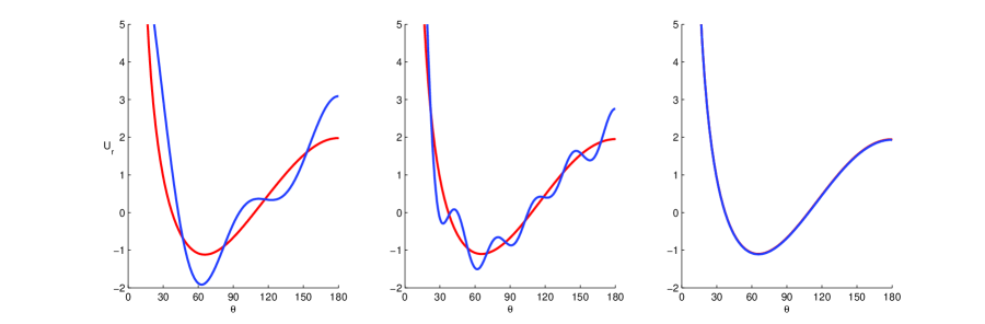
Figure 5. Comparison of the proposed solution (eq. (35) shown in red) and existing series solutions (eq. (6) shown in blue) for $U_{r}=\frac{-8\pi GR}{F}u_{r}$ under a Hertzian-type load distributed up to $\phi=10^{\circ}$. Left to right: N=4, 10, 100.

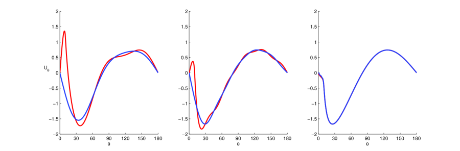
Figure 6. Comparison of the proposed solution (eq. (35) shown in red) and existing series solutions (eq. (6) shown in blue) for $U_{\theta}=\frac{-8\pi GR}{F}u_{\theta}$ under a Hertzian-type load distributed up to $\phi=10^{\circ}$. Left to right: N=4, 10, 100.

Figure 7. Convergence of the expressions for $U_{r}=\frac{-8\pi GR}{F}u_{r}$ and $U_{\theta}=\frac{-8\pi GR}{F}u_{\theta}$ given in equation (24) with $N$ for a constant distributed load given by (36). The load was distributed up to $\phi_{0}=10^{\circ}$.

4.1.1. Removing the singularity under the load

The function $S(\theta,\phi)$ exhibits a logarithmic singularity by virtue of the asymptotic behavior

$$K(m)=\log\frac{4}{\sqrt{1-m}}+\text{O}(1-m),\ \ \ m\uparrow 1.$$ (30)

The integral in (24) is evaluated by rewriting eq. (24) in the equivalent form

$$u_{r}(R,\theta)= \frac{R}{4G}\Big{\{}\int_{0}^{\phi_{0}}\Big{[}\big{(}a_{01}(\nu)S_{01}(\theta,\phi)+f(\theta,\phi)\big{)}\,\sigma(\phi)$$

$$+4(1-\nu)\big{(}S(\theta,\phi)\sigma(\phi)-\hat{S}(\theta,\phi)\sigma(\theta)\big{)}\Big{]}\sin\phi d\phi$$

$$+4(1-\nu)\sigma(\theta)\int_{0}^{\phi_{0}}\hat{S}(\theta,\phi)\sin\phi d\phi\Big{\}},\ \ 0\leq\theta\leq\phi_{0},$$ (31)

where the angle $\phi_{0}$ defines the domain of the loading, which is normally for contact problems, much less that $\pi$. The function $\hat{S}(\theta,\phi)$ has the same singularity as $S(\theta,\phi)$ and has a relatively simple integral. We choose

$$\hat{S}(\theta,\phi)=\begin{cases}-\frac{1}{2\pi}\csc\frac{\theta}{2}\sec\frac{\phi}{2}\,\log(\cos^{2}\tfrac{\phi}{2}-\cos^{2}\tfrac{\theta}{2}),&\theta>\phi,\\ -\frac{1}{2\pi}\sec\frac{\theta}{2}\csc\frac{\phi}{2}\,\log(\sin^{2}\tfrac{\phi}{2}-\sin^{2}\tfrac{\theta}{2}),&\theta<\phi,\end{cases}$$ (32)

The integrand of the first integral in (4.1.1) is now a smoothly varying function with no singularity, and the second integral is, explicitly,

$$\int_{0}^{\phi_{0}}\hat{S}(\theta,\phi)\sin\phi d\phi= -\frac{2}{\pi\sin\frac{\theta}{2}}\int_{\cos\frac{\theta}{2}}^{1}\log(x^{2}-\cos^{2}\tfrac{\theta}{2})dx-\frac{2}{\pi\cos\frac{\theta}{2}}\int_{\sin\frac{\theta}{2}}^{\sin\frac{\phi_{0}}{2}}\log(x^{2}-\sin^{2}\tfrac{\theta}{2})dx$$

$$= \frac{G(\cos\tfrac{\theta}{2},1)}{\sin\frac{\theta}{2}}+\frac{G(\sin\tfrac{\theta}{2},\sin\tfrac{\phi_{0}}{2})}{\cos\frac{\theta}{2}},\ \ 0\leq\theta\leq\phi_{0},\ \quad\text{where}$$ (33)

$$G(x,y)= -\frac{2}{\pi}\big{(}(y-x)\log(y-x)+(y+x)\log(y+x)-2(y-x+x\log 2x)\big{)}.$$ (34)

In summary, the solution for $u_{r}$ with the singularity removed has the following form (see also eq. (29a) for $H_{r}(\theta,\phi)$ and eq. (4.1.1) for $G(x,y)$)

$$u_{r}(R,\theta)= \frac{R}{4G}\Big{\{}\int_{0}^{\phi_{0}}\bigg{[}H_{r}(\theta,\phi)\sigma(\phi)-\hat{H}_{r}(\theta,\phi)\sigma(\theta)\bigg{]}\sin\phi d\phi+h(\theta)\Big{\}},$$ (35)

$$\hat{H}_{r}(\theta,\phi)= 4(1-\nu)\hat{S}(\theta,\phi),$$

$$h(\theta)= 4(1-\nu)\bigg{[}\frac{G(\cos\tfrac{\theta}{2},1)}{\sin\frac{\theta}{2}}+\frac{G(\sin\tfrac{\theta}{2},\sin\tfrac{\phi_{0}}{2})}{\cos\frac{\theta}{2}}\bigg{]}\sigma(\theta).$$

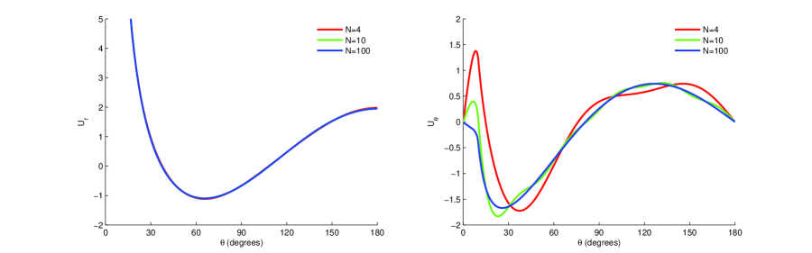
Figure 8. Convergence of the expressions for $U_{r}=\frac{-8\pi GR}{F}u_{r}$ and $U_{\theta}=\frac{-8\pi GR}{F}u_{\theta}$ given in equation (24) with $N$ for a Hertzian-type distributed load given by (37). The load was distributed up to $\phi_{0}=10^{\circ}$.

4.2. Examples of distributed loads

To check the convergence of the expressions in (24) we will consider a symmetric constant distributed load $\sigma(\phi)$ of the form

$$\sigma(\phi)=\frac{-F}{\pi R^{2}}\frac{1}{\sin^{2}\phi_{0}},\;\;\;0\leq\phi\leq\phi_{0},$$ (36)

and a symmetric Hertzian-type load of the form

$$\sigma(\phi)=\frac{-3F}{2\pi R^{2}}\frac{\sqrt{\sin^{2}\phi_{0}-\sin^{2}\phi}}{\sin^{3}\phi_{0}},\;\;\;0\leq\phi\leq\phi_{0}.$$ (37)

Both loads have been normalized such that their resultant forces are $-F$ for all ranges of the angle $\phi_{0}$, which is equivalent to the point force given by equation (7). The solution on the interval $0\leq\theta\leq\phi_{0}$ is obtained using (35) and for $\phi_{0}<\theta\leq\pi$ we apply equations (29) directly.

Firstly, the convergence of the proposed solution (eq. (35)) is compared to the series solution for a Hertzian-type load in Figures 5 and 6. These curves indicate that the convergence of the radial displacement $U_{r}$ in the proposed solution is substantially superior to the series solution. Figures 7 and 8 show the convergence of the displacements with the truncation limit $N$ under both types of loading. Subsequently, Figures 9 and 10 demonstrate that in the limit as $\phi_{0}\to 0$ the displacements due to the distributed loads approach those obtained for the point load. Moreover, the normalized radial displacement, $U_{r}$, is almost indistinguishable from the point load for a $\phi_{0}$ as large as 10 degrees. Poisson’s ratio of $\nu$=0.4 has been used throughout.

We would also like to investigate how the displacement due to a Hertzian-type load compares with that from the Hertzian contact theory. The dimensionless vertical displacement that we obtain by the methods outlined in this paper has the form

$$U_{z}=U_{r}\cos\theta-U_{\theta}\sin\theta=(8\pi GR)\frac{u_{z}}{F},$$ (38)

where $u_{z}$ is the physical vertical displacement.

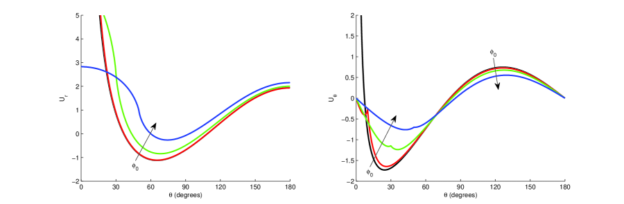
Figure 9. Comparison of the displacement due to a constant distributed load to the displacement due to a point force of the same magnitude (black). The solution was truncated at $N$=300. The loads were distributed over $\phi_{0}$=$10^{\circ}$(red), $30^{\circ}$(green), $50^{\circ}$(blue).

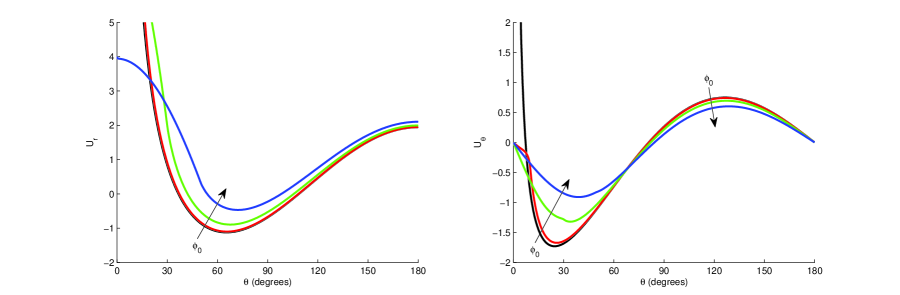
Figure 10. Convergence of the displacement due to a Hertzian-type distributed load to the displacement due to a point force of the same magnitude (black). The solution was truncated at $N$=300. The loads were distributed over $\phi_{0}$=$10^{\circ}$(red), $30^{\circ}$(green), $50^{\circ}$(blue).

The Hertz contact theory [10] is formulated in terms of the radius of the contact area $a$, the displacements directly under the load $\delta$, and the magnitude of the applied load $F$. We need to reformulate these quantities in terms of the contact angle $\phi_{0}$. The radius of the contact area is simply

$$a=R\sin\phi_{0}.$$ (39)

The maximum vertical displacement is related to $a$ in the following manner

$$\delta=\frac{a^{2}}{R}=R\sin^{2}\phi_{0}=2u_{z}(0),$$ (40)

where eq. (39) was used and the last equality arises from the fact that the Hertzian solution presented here is for the contact of two spheres hence we need to half the total displacement. Furthermore, Hertz contact theory tells us that the resultant force $F$ is proportional to $a^{3}$, or more accurately

$$F=\frac{4}{3}\Big{(}\frac{G}{1-\nu}\Big{)}\frac{a^{3}}{R}=\frac{4}{3}\Big{(}\frac{G}{1-\nu}\Big{)}R^{2}\sin^{3}\phi_{0}.$$ (41)

This allows to rewrite equation (38) for the dimensionless vertical displacement via Hertz contact theory, denoted as $U_{z}^{H}(0)$. Substituting equations (40) and (41) into (38) yields

$$U_{z}^{H}(0)=(8\pi GR)\frac{\frac{R}{2}\sin^{2}\phi_{0}}{\frac{4}{3}\big{(}\frac{G}{1-\nu}\big{)}R^{2}\sin^{3}\phi_{0}}=\frac{3\pi(1-\nu)}{\sin\phi_{0}}.$$ (42)

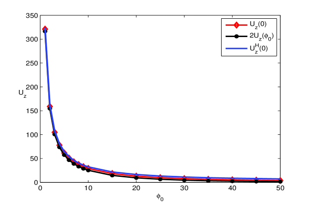
Figure 11. Comparison of the dimensionless vertical displacement $U_{z}=(8\pi GR)\frac{u_{z}}{F}$ as obtained by the methods in this paper for a Hertzian-type load and that obtained from Hertz contact theory $U_{z}^{H}$ defined in (42), as a function of the contact angle $\phi_{0}$.

Equation (42) gives a way to compare the presented solution for the Hertzian-type load to the solution from Hertz contact theory. The numerical results are presented in Figure 11, which compares the vertical displacements (eq. (38) with eq. (42)) as a function of the contact angle $\phi_{0}$. Note that along with $U_{z}(0)$ and $U_{z}^{H}(0)$ we also plot $2U_{z}(\phi_{0})$, which according to Hertz theory should be equal to $U_{z}(0)$. The normalized difference between the displacements is shown in Figure 12. As expected, the solutions are close for small contact areas and diverge as this area increases. The same can be said about the relationship between the displacements $U_{z}(0)$ and $2U_{z}(\phi_{0})$.

Comparing the maximum displacements $U_{z}(0)$ with $U_{z}^{H}(0)$ does not tell us anything about the shape of the contact area for a sphere loaded by a Hertzian-type load. Hertz contact theory states that the contact area between two identical spheres is flat, and thus we can describe it using $R(\cos\theta-\cos\phi_{0})$. Therefore, we define a function $s(\theta)$ to determine how close is our calculated displacement to the Hertzian solution as

$$s(\theta)=kU_{z}(\theta)-(\cos\theta-\cos\phi_{0}),$$ (43)

where $k$ is a constant determined by enforcing $s(0)=s(\phi_{0})$, which results in

$$s(\theta)=\frac{U_{z}(\theta)}{U_{z}(0)-U_{z}(\phi_{0})}(1-\cos\phi_{0})-(\cos\theta-\cos\phi_{0}).$$ (44)

The function $s(\theta)$ is plotted in Figure 13 for several angles $\phi_{0}$. These results show that the contact area is flat for small contact angles, but gains curvature for larger angles. According to Hertz theory, for small contact angles $\phi_{0}$, the function $s(\theta)$ behaves as a constant $s(\theta)\approx\phi_{0}^{2}/2$. The angles shown in Figure 13 are too large to see this behaviour, however, at $\phi_{0}=5^{\circ}$ the values are close with $s(\theta)=0.00334$ and $\phi_{0}^{2}/2=0.00381$.

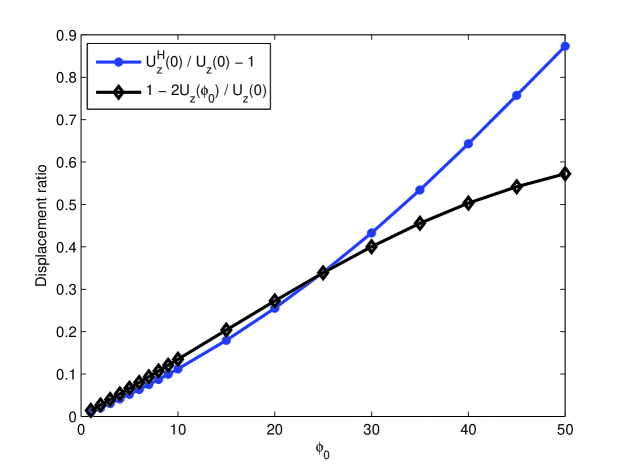
Figure 12. Normalized difference between the displacements in Figure 11 as a function of the contact angle $\phi_{0}$.

5. Conclusions

A compact Green’s function for a sphere is presented which uses the fundamental idea of expressing a slowly convergent series with analytical functions and a quickly convergent series. The increased speed of convergence is demonstrated for the point force solution, which is also shown to be consistent with the more general distributed loading in the limit as the contact angle approaches zero. Since the general Green’s function contains elliptical integrals, an easy method for dealing with the singularity in the integrand is presented. Comparing the exact displacement due to a Hertzian-type distributed load to the displacement given by Hertz contact theory we conclude that the Hertz contact theory gives accurate results for contact angles up to about $10^{\circ}$, with a steadily increasing error. For larger contact angles, Hertz theory overestimates the displacements and cannot account for the shape of the contact area. This is to say that the stress distribution assumed in Hertz theory results in a curved contact surface for larger contact angles.

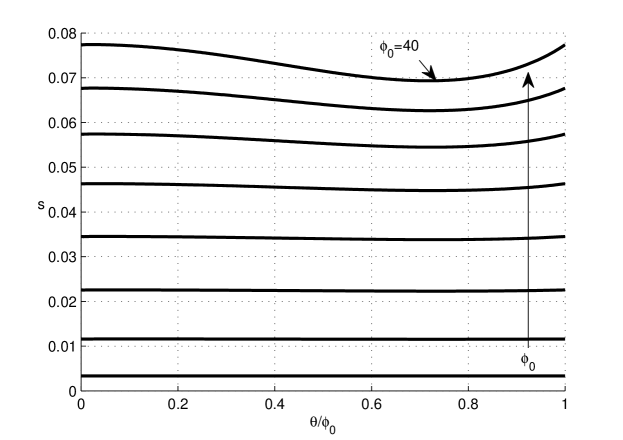
Figure 13. The flatness of the area under the load as defined in eq. (44) as a function of the normalized angle $\theta/\phi_{0}$. Each curve corresponds to a different contact angle ranging from $\phi_{0}=5^{\circ}$ to $40^{\circ}$ in $5^{\circ}$ increments.

Appendix A: Legendre polynomial formulas

The orthogonality and completeness relations for the Legendre functions are

$$\frac{1}{2}{(2n+1)}\int\limits_{0}^{\pi}P_{m}(\cos\theta)P_{n}(\cos\theta)\,\sin\theta\,d\theta =\delta_{mn},$$ (45a)

$$\sum\limits_{n=0}^{\infty}\frac{1}{2}(2n+1)P_{n}(\cos\theta)P_{n}(\cos\phi) =\frac{\delta(\theta-\phi)}{\sin\phi},$$ (45b)

Starting with the definition for $P_{n}(x)$,

$$P_{n}(\cos\theta)=\frac{1}{\pi}\int_{0}^{\pi}(\cos\theta+i\sin\theta\cos\alpha)^{n}\,d\alpha,$$ (46)

and using $\sum\limits_{n=0}^{\infty}z^{n}=\frac{1}{1-z}$, $|z|<1$, the well known generating function follows

$$\sum\limits_{n=0}^{\infty}{t}^{n}P_{n}(\cos\theta)=\frac{1}{\sqrt{1+t^{2}-2t\cos\theta}},\ \ |t|\leq 1.$$ (47)

Integrating the identity (47) with respect to $t$ implies

$$\sum\limits_{n=0}^{\infty}t^{n+1}\frac{P_{n}(\cos\theta)}{n+1}=\sinh^{-1}(\cot\theta)+\sinh^{-1}\bigg{(}\frac{t-\cos\theta}{\sin\theta}\bigg{)}$$

$$\quad=\log\big{(}1+\csc\frac{\theta}{2}\big{)}-\sinh^{-1}(\tan\frac{\theta}{2})+\sinh^{-1}\Big{(}\frac{t-\cos\theta}{\sin\theta}\Big{)},\ \ |t|\leq 1,\ \ 0\leq\theta\leq\pi.$$ (48)

Taking the limit as $t\to 1$ yields (12a). $S_{1}(\theta)$ of (12b) follows from a similar result [11, eq. 5.10.1.4], while $S_{2}(\theta)$ of (12c) follows from the recurrence relation

$$(n+1)P_{n+1}(x)-(2n+1)xP_{n}(x)+nP_{n-1}(x)=0,$$ (49)

after dividing by $n$ and summing from $n=1$ to $\infty$ ($S_{2}$ agrees with [11, eq. 5.10.1.6]). The recurrence relation can be used to then find $S_{j}(\theta)$ for $j=3$, $4,\ldots$.

Series of products of Legendre functions given by eqs. 6.11.3.1 and 6.11.3.2 of [12]

$$\sum\limits_{n=1}^{\infty}\frac{2n+1}{n(n+1)}P_{n}(x)P_{n}(y) =-1-\log\tfrac{(1-x)(1+y)}{4},$$ (50)

$$\sum\limits_{n=1}^{\infty}\frac{2n+1}{n^{2}(n+1)^{2}}P_{n}(x)P_{n}(y) =1-\log\tfrac{1+y}{2}\log\tfrac{(1-x)(1+y)}{4}+Li_{2}\big{(}\tfrac{1+x}{2}\big{)}-Li_{2}\big{(}\tfrac{1+y}{2}\big{)},$$

for $-1\leq x<y\leq 1$. Equation (50)₁ can be derived by operating on both sides by the Legendre differential operator $L_{x}=\frac{d}{dx}(1-x^{2})\frac{d}{dx}$, and using the eigenvalue property $L_{x}P_{n}(x)=-n(n+1)P_{n}(x)$ to arrive at (8b) (for $x<y$). At the same time, the constants in the right member of (50)₁ follow by considering the formula for $x=0$, $y=1$ in which case the sum on the left can be found. Equation (50)₁ gives $S_{0}(\theta,\phi)+S_{1}(\theta,\phi)$ by noting that $\frac{1}{n}+\frac{1}{n+1}=\frac{2n+1}{n(n+1)}$.

The following is a simple consequence of Legendre’s addition formula [13, eq. 3.19]

$$P_{n}(\cos\theta)P_{n}(\cos\phi)=\frac{1}{\pi}\int_{0}^{\pi}P_{n}(\cos\theta\cos\phi-\sin\theta\sin\phi\cos\alpha)\,d\alpha.$$ (51)

Multiply both sides of (51) by $t^{n}$ and sum, implies, using eq. (47), the identity [11, eq. 5.10.2.1] for $|t|<1$,

$$\sum\limits_{n=0}^{\infty}t^{n}\,P_{n}(\cos\theta)P_{n}(\cos\phi)=\frac{4}{\pi(u_{+}+u_{-})}\,K\Big{(}\frac{u_{+}-u_{-}}{u_{+}+u_{-}}\Big{)},\\ u_{\pm}=\sqrt{1-2t\cos(\theta\pm\phi)+t^{2}}.$$ (52)

Appendix B: Analytical functions and their derivatives

We require the derivatives with respect to $\theta$ of the functions defined in eq. (12). They are

$$\frac{dS_{0}(\theta)}{d\theta} =\frac{\sin\frac{\theta}{2}-1}{\sin\theta},$$ (53)

$$\frac{dS_{1}(\theta)}{d\theta} =-\frac{dS_{0}(\theta)}{d\theta}-\cot\frac{\theta}{2},$$

$$\frac{dS_{2}(\theta)}{d\theta} =\frac{dS_{1}(\theta)}{d\theta}\cos\theta-S_{1}(\theta)\sin\theta+\cos\frac{\theta}{2}\Big{(}2\sin\frac{\theta}{2}-1\Big{)}.$$

Similarly, the analytical function used to find $u_{\theta}$ (eq. (29)) in section 4 is

$$S_{01}(\theta,\phi)=S_{0}(\theta,\phi)+S_{1}(\theta,\phi)=\begin{cases}-2\log\sin\frac{\theta}{2}\cos\frac{\phi}{2},&\theta>\phi,\\ -2\log\cos\frac{\theta}{2}\sin\frac{\phi}{2},&\theta<\phi.\end{cases}$$ (54)

The derivative of $S_{01}(\theta,\phi)$ is

$$\frac{\partial S_{01}(\theta,\phi)}{\partial\theta}=\begin{cases}-\cot\frac{\theta}{2},&\theta>\phi,\\ \tan\frac{\theta}{2},&\theta<\phi.\end{cases}$$ (55)

References

- [1] H. Hertz. Ueber die berührung fester elastischer körper. Jornal für die Reine und Angewandte Mathematik, 92:156–171, 1881.
- [2] E. Sternberg and F. Rosenthal. The elastic sphere under concentrated loads. 19:413–421, 1952.
- [3] I. Guerrero and M. J. Turteltaub. The elastic sphere under arbitrary concentrated surface loads. 2(1):21–33, 1972.
- [4] V. Bondareva. On the effect of an axisymmetric normal loading on an elastic sphere. J. Appl. Math. Mech., 33(6):1001–1005, 1969.
- [5] V. Bondareva. Contact problems for an elastic sphere. J. Appl. Math. Mech., 35(1):37–45, 1971.
- [6] P. Villaggio. The rebound of an elastic sphere against a rigid wall. 63(2):259–263, 1996.
- [7] A. I. Lur’e. Three-dimensional Problems of the Theory of Elasticity. Gostekhizdat, Moscow, 1955.
- [8] O. I. Zhupanska. Contact problem for elastic spheres: Applicability of the Hertz theory to non-small contact areas. 49:576–588, 2011.
- [9] M. Abramowitz and I. Stegun. Handbook of Mathematical Functions with Formulas, Graphs, and Mathematical Tables. Dover, New York, 1974.
- [10] K. L. Johnson. Contact Mechanics. Cambridge University Press, Cambridge, UK, 1985.
- [11] A. P. Prudnikov, Yu. A. Brychko, O. I. Marichev, and N.M. Queen. Integrals and Series. Vol. 2: Special Functions. Gordon and Breach, New York, 1986.
- [12] Yu. A. Brychko. Handbook of Special Functions: Derivatives, Integrals, Series and Other Formulas. CRC Press, 2008.
- [13] P. A. Martin. Multiple Scattering: Interaction of Time-harmonic Waves with N Obstacles. Cambridge University Press, New York, 2006.