STEP POTENTIALS FOR DARK ENERGY

Abstract

We consider a reconstructing scheme using observational data from SNIa, BAO and CMB, based on a model of dark unification using a single non-minimally coupled scalar field. We investigate through a reconstruction program, the main features the current observational data imposes to the scalar field potential. We found that the form suggested by observations implies a step feature in the potential, where the kinetic and potential energy becomes of the same order of magnitude.

I Introduction

Dark energy is the name of the unknown component responsible for the current accelerated expansion of the universe dereview . In its simpler form, this can be described by a fluid with constant equation of state parameter $w=-1$, corresponding to a cosmological constant, leading to the successful $\Lambda$CDM model, the simplest model that fits a varied set of observational data.

This model posses a high dependence to initial conditions that makes it unnatural in many ways. For example, the current value for $\Omega_{\Lambda}$ and $\Omega_{M}$ are of the same order of magnitude, a fact highly improbable, because the dark matter contribution decreases with $a^{-3}$, with $a(t)$ the scale factor, meanwhile the cosmological constant contribution have had the same value always. This problem in particular is known as the cosmic coincidence problem.

In this context, the most natural way to understand the acceleration of the universe, is to assume the existence of a dynamical cosmological constant, or a theoretical model with a dynamical equation of state parameter ($p/\rho=w(z)$). The source of this dynamical dark energy could be both, a new field component filling the universe, as a quintessence scalar field quinta , or it can be produced by modifying gravity modgrav .

In Shafieloo:2009ti the authors suggested that the current observational data favor a scenario in which the acceleration of the expansion has past a maximum value and is now decelerating. The key point in deriving this conclusion is the use of the Chevalier-Polarski-Linder (CPL) parametrization Chevallier:2000qy , Linder:2002et for a dynamical equation of state parameter

$$w(a)=w_{0}+(1-a)w_{1},$$ (1)

where $w_{0}$ and $w_{1}$ are constants to be fixed by observations and $a$ is the scale factor. An update analysis performed using recent SNIa data was informed in Li:2010da where similar conclusions were derived. Both analysis assume a flat universe.

In Cardenas:2011a , we study the previous model, using a new set of data, the Union 2 data set Union2 , and also considering the possibility to incorporate the curvature parameter $\Omega_{k}$, as a new free parameter in the analysis. We find that, the three observational test; SNIa, BAO and CMB, all can be accommodated in the same trend, assuming a very small value for the curvature, $\Omega_{k}\simeq-0.08$. The best fit values suggest that the acceleration of the universe has already reached its maximum, and is currently moving towards a decelerating phase.

Using a scalar field to model dark energy, it is possible to reconstruct the scalar field potential from observations. There are many approaches to do this Sahni:2006pa . Considering models of a single non-minimally coupled scalar field, the rapid variations of the equation of state parameter at low redshift can not be described.

The quest for the unification of inflation, dark matter, and dark energy, in different combinations, by a single field, has been studied in Refs. Peebles:1998qn ; Lidsey:2001nj ; Padmanabhan:2002sh ; Scherrer:2004au ; Matos:2005yt ; Arbey:2006it ; Cardenas:2006py ; Cardenas:2007xh ; Panotopoulos:2007ri ; Liddle:2006qz ; Liddle:2008bm ; Bose:2009kc ; BasteroGil:2009eb ; DeSantiago:2011qb . The main motivation behind all proposals is that we do not yet understand the nature of the components responsible for the three phenomena, but we do know that their special properties are beyond the realm of the ordinary matter described by the Standard Model of Particle Physics.

An extreme, most economical, possibility is that all three phenomena can be explained by the existence of one single field. As was first put forward in Ref. Liddle:2006qz ; Liddle:2008bm , the simplest option at hand is a scalar field $\phi$ with a potential of the form $V(\phi)=V_{0}+(1/2)m^{2}\phi^{2}$. The energy scale $V_{0}$ is to be set at the tiny value of the observed cosmological constant considered in the concordance $\Lambda$CDM model, and the mass scale of the field, $m\simeq 10^{-6}m_{\rm pl}$, is determined by the amplitude of primordial perturbations generated during inflation.

It is the purpose of this paper to explore the consequences of this trend, suggested from the observations, and look for special features through a characterization of a unification model based on a scalar field, that allows these transitions at low redshift. The reconstruction program uses as an intermediate phase a certain parametrization of $w(z)$, which after its test using the data, is slightly altered looking for improvements in the fit. Here we use a $\chi^{2}$ test considering the AIC and BIC criteria that controls the number of parameters to be used.

II $w(z)$ from the observations

The problem of extracting information of $w(z)$ from observations can be understand in the following way. Because most of the measurements give us information of the Hubble function $H(z)$ or also the luminosity (or angular diameter) distance $d_{L}(z)$, we are forced to use

$$w(z)=-\frac{1}{3}\frac{2(1+z)HH^{\prime}-3H^{2}}{H_{0}^{2}(1+z)^{3}\Omega_{m}-H^{2}},$$ (2)

in the case of data from $H(z)$, and we are forced to use

$$w(z)=-\frac{1}{3}\left(\frac{2(1+z)D^{\prime\prime}+3D^{\prime}}{D^{\prime}-(D^{\prime})^{3}\Omega_{m}(1+z)^{3}}\right),$$ (3)

in the case of the luminosity distance, where $D\equiv H_{0}d_{L}(z)/c$. Notice that the precision in values for $\Omega_{m}$ and $\Omega_{k}$ are crucial in this reconstruction procedure.

The limitations of this process, first identified in Maor:2000jy , are related to the dependence of the function $w(z)$ of first and second derivatives of the $H(z)$ and $D(z)$ functions respectively. In order to tackle this problem, we can try to model the $w(z)$ shape, by using a proper parametrization. The most used is the already mentioned CPL Chevallier:2000qy , Linder:2002et , but there are many others designed to specific goals. For example, to describe a fast transition at redshift $z_{t}$ we can use

$$w(z)=w_{i}+\frac{w_{f}-w_{i}}{1+\exp(\frac{z-z_{t}}{\delta})}$$

or if we are interested in oscillatory behaviour we can use

$$w(z)=w_{0}+w_{1}\cos\left(A\log\frac{1+z_{c}}{1+z}\right).$$

However, there is a concern regarding the number of parameters used to parameterize $w(z)$. It is clear that increasing the number of parameters Liddle:2004nh , is easiest to improve the fit with observations, but is not clear if in the meantime we are adjusting noise, instead of the truly physical relation.

III The approach

In this section we describe the method to reconstruct the scalar field potential through the use of a iterative program improving the fit using two parameterizations for the equation of state parameter $w(z)$. In this section we assume that $\Omega_{k}=0$.

The comoving distance from the observer to redshift $z$ is given by

$$r(z)=\frac{c}{H_{0}}\int_{0}^{z}\frac{dz^{\prime}}{E(z^{\prime})},$$ (4)

where

$$E^{2}(z) = \Omega_{m}(1+z)^{3}+\Omega_{de}f(z),$$ (5)

$$f(z) = \exp\left\{3\int^{z}_{0}\frac{1+w(z^{\prime})}{1+z^{\prime}}dz^{\prime}\right\},$$

and $\Omega_{de}=1-\Omega_{m}$. The SNIa data give the luminosity distance $d_{L}(z)=(1+z)r(z)$. We fit the SNIa with the cosmological model by minimizing the $\chi^{2}$ value defined by

$$\chi_{SNIa}^{2}=\sum_{i=1}^{557}\frac{[\mu(z_{i})-\mu_{obs}(z_{i})]^{2}}{\sigma_{\mu i}^{2}},$$ (6)

where $\mu(z)\equiv 5\log_{10}[d_{L}(z)/\texttt{Mpc}]+25$ is the theoretical value of the distance modulus, and $\mu_{obs}$ is the corresponding observed one.

The BAO data considered in our analysis is the distance ratio obtained at $z=0.20$ and $z=0.35$ from the joint analysis of the 2dF Galaxy Redsihft Survey and SDSS data bao2 , that can be expressed as

$$\frac{D_{V}(0.35)}{D_{V}(0.20)}=1.736\pm 0.065,$$ (7)

with

$$D_{V}(z_{BAO})=\bigg{[}\frac{z_{BAO}}{H(z_{BAO})}\bigg{(}\int_{0}^{z_{BAO}}\frac{dz}{H(z)}\bigg{)}^{2}\bigg{]}^{1/3}.$$ (8)

We fit the cosmological model minimizing the $\chi^{2}$ defined by

$$\chi_{BAO}^{2}=\frac{[D_{V}(0.35)/D_{V}(0.20)-1.736]^{2}}{0.065^{2}}.$$ (9)

A result from the combination of SNIa and BAO is given by a joint analysis finding the best fit parameters that minimize $\chi_{SNIa}^{2}+\chi_{BAO}^{2}$.

In addition, we can incorporate to the analysis the CMB redshift parameter cmb2 , which is the reduce distance at $z_{ls}=1090$ Wang:2007mza

$$R=\sqrt{\Omega_{m}H_{0}^{2}}r(z_{ls})=1.71\pm 0.019.$$ (10)

We also apply the $\chi^{2}$

$$\chi^{2}_{CMB}=\frac{[R-1.71]^{2}}{0.019^{2}}\;,$$ (11)

to find out the result from CMB and the constraints from SNIa+BAO+CMB are given by $\chi_{SNIa}^{2}+\chi_{BAO}^{2}+\chi_{CMB}^{2}$.

Assuming a form for $w(z)$ in terms of a certain number of parameters, we perform a Bayesian analysis to obtain the best fit values of all the free parameters in the model.

IV The CPL case

For example, using the CPL parametrization, $w=w_{0}+w_{1}z/(1+z)$, the function defined in (5) leads to

$$f(z)=(1+z)^{3(1+w_{0}+w_{1})}\exp\left(-\frac{3w_{1}z}{1+z}\right).$$ (12)

Using the Union 2 set Union2 , consisting in $557$ type Ia supernovae, the analysis leads to the results shown in Table 1.

Table 1: The best fit values for the free parameters using the Union 2 data set in the case of a flat universe model.

Data Set	$\chi^{2}_{min}$	$\Omega_{m}$	$w_{0}$	$w_{1}$
SN	541.43	0.4197	-0.8632	-5.490
SN+BAO	542.11	0.4281	-0.7959	-6.537
SN+BAO+CMB	543.91	0.2547	-0.9979	0.190

A plot of the deceleration parameter using these numbers is shown in Fig.1.

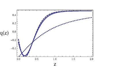
Figure 1: Using the Union 2 data set we plot the deceleration parameter reconstructed using the best fit values for three cases: only SNIa (continuos line), SNIa+BAO (dashed line) and SNIa+BAO+CMB (dotted line)

Figure 2: The confidence limits for the case of Fig.1

The case SNIa alone and SNIa+BAO are almost identical, but the case including CMB data does not show the rapid change at small redshift. Using the best fit values for the parameters, give us the best fit function $H(z)$ that we can use to reconstruct the scalar field potential. Using a standard procedure Cardenas:2004ji with the equations for the flat case

$$\phi^{\prime}(z)^{2} = \frac{1}{4\pi G}\frac{H^{\prime}}{(1+z)H},$$ (13)

$$V(z) = \frac{3}{8\pi G}\left[H^{2}-\frac{(1+z)HH^{\prime}}{3}\right],$$ (14)

we can plot directly the scalar field potential. In Fig.3 we show the integration of these relations. As is expected, in the cases SNIa and SNIa+BAO, we observe a rapid change in slope, a “knee” feature, that is not observed in the case including CMB.

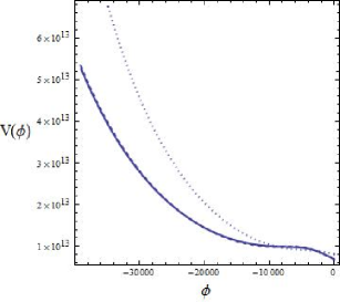
Figure 3: Using the Union 2 data set we plot the scalar field potential reconstructed using the best fit function $H(z)$ for the three cases: only SNIa (continuos line), SNIa+BAO (dashed line) and SNIa+BAO+CMB (dotted line). The first two overlap almost exactly.

Then the sharp change observed in the reconstructed deceleration parameter $q(z)$ suggested by the data, is here visible in the scalar field potential $V(\phi)$ as this knee feature Wang:2009av .

This is the anomalous effect mentioned first in Shafieloo:2009ti using the Constitution data set for SNIa, and also in Li:2010da and Cardenas:2011a . A large negative value for $w_{1}$ means that for small redshift the data suggest a negative slope for $w(z)$. Because we are using the CPL parametrization, this fact spoils the large $z$ behavior of the EoS parameter, leading to a large negative values $w(z\rightarrow\infty)\simeq-7$.

This is the kind of small redshift transitions in $w(z)$ that were discussed first in Bassett:2002qu and also in Mortonson:2009qq . In Bassett:2002qu they use a form,

$$w(z)=w_{0}+\frac{w_{f}-w_{0}}{1+\exp((z-z_{t})/\Delta)},$$ (15)

that captures the essence of a single transition at $z_{t}$ in a range $\Delta$, from $w_{0}$ initially to a final value $w_{f}$ in the future. In Mortonson:2009qq the authors discussed the possibility of a fast change in $w(z)$ at $z<0.02$ and its implication for a standard scalar field model. They found that while a canonical scalar field model can decrease the expansion rate at low redshift, increasing the local expansion rate requires a non-canonical kinetic term for the scalar field.

In this work we present an analysis of this problem using real data, as opposite to the previous analysis, to constraint the form of the equation of state parameter $w(z)$ and then through relations (13) to constraint the scalar field potential $V(\phi)$ in a unified dark matter dark energy model.

V Improving the fit

As is evident from the previous section, the results show the incompatibility of the CPL parametrization in describing the variation of $w(z)$ with redshift, because the data suggest a very large and negative value for $w_{1}$ which spoils the large $z$ behavior of $w(z)$.

In order to improve the fit, some authors have suggested the use of a new parametrization Shafieloo:2009ti for $w(z)$. We can use for example, the fast single transition form (15), to improve the fit. However, this parametrization has four parameters, two more than the CPL. Adding a new parameter would be justifiable only if the AIC or BIC (or a combination of these two) numbers indicate so Liddle:2004nh . In this context, if we do not have new insight, we would like to keep the number of parameters fixed (in this case two), until one of these numbers (AIC or BIC) indicated something else.

Let us start with a first iteration of the process. The negative value for $w_{1}$ obtained in the previous section indicate that $w(z)$ has to change its slope recently, and as the CPL reproduce perfectly, at large $z$ its value does not change very much. So, let us use the following ansatz for $w(z)$:

$$w(z)=-\frac{w_{0}}{1+z}+\frac{w_{1}}{(1+z)^{2}}.$$ (16)

This form has two parameters, like the CPL, so they are both directly comparable with $\chi^{2}$ statistic, and also this has a dust limit for $z\rightarrow\infty$. The main feature of this parametrization is that allows the possibility to describe a change of $w(z)$ at low $z$, without spoiling the large $z$ behavior. The result of a bayesian analysis is displayed in Table 2.

Table 2: The best fit values for the free parameters of the parametrization (16) using the Union 2 data set for SNIa, in a flat universe model.

Data Set	$\chi^{2}_{min}$	$\Omega_{m}$	$w_{0}$	$w_{1}$
N	541.32	0.4121	8.7568	7.990
SN+BAO	542.11	0.4281	-0.7959	-6.537
SN+BAO+CMB	543.91	0.2547	-0.9979	0.190

Notice that, although the deceleration parameter obtained from SNIa and SNIa+BAO still remains very close each other, meanwhile that considering CMB behaves differently, the curve for the joint analysis SNIa+BAO+CMB shows a change in slope close to $z=0$ that is not observed using CPL.

Figure 4: The same as Fig.1

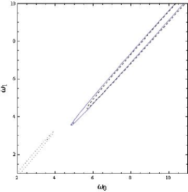
Figure 5: The same as Fig.3

The second panel also shows this slight improvement, although still remains the conflict between low and high redshift data. The performance of this new parametrization is displayed in Table 3.

Table 3: A summary of the performance using CPL and the new parametrization using only SNIa data. We display also the AIC and BIC indexes to compare with the $\Lambda$CDM fit.

SNIa	$k$	$-2\ln\textsl{L}$	$\triangle$AIC	$\triangle$BIC
$\Lambda$CDM	2	542.63	0	0
CPL	3	541.43	0.80	-1.2
New	3	541.32	0.69	-1.31

Clearly, our new parametrization is an improvement respect to CPL. The best fit parameters suggest a step like feature in the potential, as we can see in Fig. 6. We can still look for a better parametrization trying to accommodate all the three observational probes in a single trend.

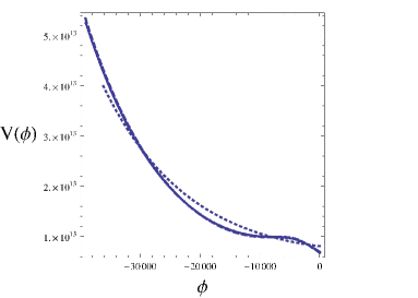
Figure 6: The same as Fig. 3. Notice the improvement having all the curves overlap but still show a distinc behavior once we consider the CMB data.

VI Results

In this paper we investigate the consequences of the low redshift variations in the equation of state parameter, suggested by the data, and their implications in a unified scalar field model for dark matter and dark energy. This trend suggest a special feature in the scalar field potential. The reconstruction program uses as an intermediate phase a parametrization of $w(z)$, which after its test using the data, is slightly altered looking for improvements in the fit. Here we have used a $\chi^{2}$ test considering the AIC and BIC criteria that controls the number of parameters to be used. We found a better parametrization than the CPL, that properly describe the low redshift behaviour, but although ameliorate the tension between low and high redshift, it can not describe all the data together.

References

- (1) M. Sami, arXiv: 0904.3445 [hep-th]; J. Frieman, M. Turner and D. Huterer, Ann. Rev. Astron. Astrophys. 46, 385 (2008); T. Padmanabhan, Gen. Rel. Grav. 40, 529 (2008); M.S. Turner and D. Huterer, J. Phys. Soc. Jap. 76, 111015 (2007); N. Straumann, Mod. Phys. Lett. A21 1083 (2006); E.J. Copeland, M. Sami and S. Tsujikawa, Int. J. Mod. Phys. D 15, 1753 (2006).
- (2) C. Wetterich, Nucl. Phys. B 302, 668 (1988); B. Ratra and P.J.E. Peebles, Phys. Rev. D 37, 3406 (1988); J.A. Frieman, C.T. Hill, A. Stebbins and I. Waga, Phys. Rev. Lett. 75, 2077 (1995) ; M.S. Turner and M. White, Phys. Rev. D 56, R4439 (1997); R.R. Caldwell, R. Dave and P.J. Steinhardt, Phys. Rev. Lett. 76, 1582 (1998); A.R. Liddle and R.J. Scherrer, Phys. Rev. D 59, 023509 (1999); P.J. Steinhardt, L. Wang, and I. Zlatev, Phys. Rev. D 59, 123504 (1999).
- (3) G.R. Dvali, G. Gabadadze, and M. Porrati, Phys. Lett. B485, 208 (2000); C. Deffayet, Phys. Lett. B502, 199 (2001); S. Nojiri and S. D. Odintsov, Phys. Rev. D 68, 123512 (2003); S.M. Carroll, V. Duvvuri, M. Trodden, and M.S. Turner, Phys. Rev. D70, 043528 (2004); S. Noriji and S.D. Odintsov, Int. J. Geom. Meth. Mod. Phys. 4, 115 (2007); Y.S. Song, W. Hu, and I. Sawicki, Phys. Rev. D75, 044004 (2007); S. Nojiri and S. D. Odintsov, Phys. Rev. D 77, 026007 (2008).
- (4) V. Sahni and A. Starobinsky, Int. J. Mod. Phys. D 15, 2105 (2006) [arXiv:astro-ph/0610026].
- (5) I. Maor, R. Brustein and P. J. Steinhardt, Phys. Rev. Lett. 86, 6 (2001) [Erratum-ibid. 87, 049901 (2001)] [astro-ph/0007297].
- (6) P. J. E. Peebles, A. Vilenkin, Phys. Rev. D59, 063505 (1999). [astro-ph/9810509].
- (7) J. E. Lidsey, T. Matos, L. A. Urena-Lopez, Phys. Rev. D66, 023514 (2002). [astro-ph/0111292].
- (8) T. Padmanabhan, T. R. Choudhury, Phys. Rev. D66, 081301 (2002). [hep-th/0205055].
- (9) R. J. Scherrer, Phys. Rev. Lett. 93, 011301 (2004). [astro-ph/0402316].
- (10) T. Matos, J. -R. Luevano, H. Garcia-Compean, Int. J. Mod. Phys. A23, 1949-1962 (2008). [hep-th/0511098].
- (11) A. Arbey, Phys. Rev. D74, 043516 (2006). [astro-ph/0601274].
- (12) V. H. Cardenas, Phys. Rev. D73, 103512 (2006). [gr-qc/0603013].
- (13) V. H. Cardenas, Phys. Rev. D75, 083512 (2007). [astro-ph/0701624].
- (14) G. Panotopoulos, Phys. Rev. D75, 127301 (2007). [arXiv:0706.2237 [hep-ph]].
- (15) A. RLiddle, L A. Urena-Lopez, Phys. Rev. Lett. 97, 161301 (2006). [astro-ph/0605205].
- (16) A. R. Liddle, C. Pahud, L. A. Urena-Lopez, Phys. Rev. D77, 121301 (2008). [arXiv:0804.0869 [astro-ph]].
- (17) N. Bose, A. S. Majumdar, Phys. Rev. D80, 103508 (2009). [arXiv:0907.2330 [astro-ph.CO]].
- (18) M. Bastero-Gil, A. Berera, B. M. Jackson, A. Taylor, Phys. Lett. B678, 157-163 (2009). [arXiv:0905.2937 [hep-ph]].
- (19) J. De-Santiago, J. L. Cervantes-Cota, Phys. Rev. D83, 063502 (2011). [arXiv:1102.1777 [astro-ph.CO]].
- (20) A. Shafieloo, V. Sahni and A. A. Starobinsky, Phys. Rev. D 80, 101301 (2009) [arXiv:0903.5141 [astro-ph.CO]].
- (21) M. Chevallier and D. Polarski, Int. J. Mod. Phys. D 10, 213 (2001) [arXiv:gr-qc/0009008].
- (22) E. V. Linder, Phys. Rev. Lett. 90, 091301 (2003) [arXiv:astro-ph/0208512].
- (23) B. A. Bassett, M. Kunz, J. Silk and C. Ungarelli, Mon. Not. Roy. Astron. Soc. 336, 1217 (2002) [arXiv:astro-ph/0203383].
- (24) M. Mortonson, W. Hu and D. Huterer, Phys. Rev. D 80, 067301 (2009) [arXiv:0908.1408 [astro-ph.CO]].
- (25) Z. Li, P. Wu and H. Yu, Phys. Lett. B 695, 1 (2011) [arXiv:1011.1982 [gr-qc]].
- (26) V.H. Cárdenas and M. Rivera, Phys. Lett. B 710, 251 (2012) [arXiv:1203.0984 [astro-ph.CO]].
- (27) M. Hicken et al., Astrophys. J. 700, 1097 (2009) [arXiv:0901.4804 [astro-ph.CO]].
- (28) R. Amanullah et al., Astrophys. J. 716, 712 (2010) [arXiv:1004.1711 [astro-ph.CO]].
- (29) B. A. Reid et al., Mon. Not. Roy. Astron. Soc. 404, 60 (2010) [arXiv:0907.1659 [astro-ph.CO]]; B. A. Reid et al. [SDSS Collaboration], Mon. Not. Roy. Astron. Soc. 401, 2148 (2010) [arXiv:0907.1660 [astro-ph.CO]].
- (30) G. Hinshaw et al. [WMAP Collaboration], Astrophys. J. Suppl. 180, 225 (2009) [arXiv:0803.0732 [astro-ph]]; E. Komatsu et al. [WMAP Collaboration], Astrophys. J. Suppl. 180, 330 (2009) [arXiv:0803.0547 [astro-ph]].
- (31) Y. Wang and P. Mukherjee, Phys. Rev. D 76, 103533 (2007) [arXiv:astro-ph/0703780].
- (32) L. Perivolaropoulos and A. Shafieloo, Phys. Rev. D 79, 123502 (2009) [arXiv:0811.2802 [astro-ph]].
- (33) V. H. Cardenas, S. del Campo, Phys. Rev. D69, 083508 (2004). [astro-ph/0401031].
- (34) A. R. Liddle, Mon. Not. Roy. Astron. Soc. 351, L49-L53 (2004). [astro-ph/0401198].
- (35) T. Wang, Phys. Rev. D 80, 101302 (2009) [arXiv:0908.2477 [hep-th]].