Wireless Network Stability in the SINR Model

Abstract.

We study link scheduling in wireless networks under stochastic arrival processes of packets, and give an algorithm that achieves stability in the physical (SINR) interference model. The efficiency of such an algorithm is the fraction of the maximum feasible traffic that the algorithm can handle without queues growing indefinitely. Our algorithm achieves two important goals: (i) efficiency is independent of the size of the network, and (ii) the algorithm is fully distributed, i.e., individual nodes need no information about the overall network topology, not even local information.

1. Introduction

We study the problem of scheduling packets over links in a wireless network, each link being a sender-receiver pair of wireless nodes. Since wireless signals propagate in all directions, simultaneous transmissions interfere with each other. This interference limits the number of transmissions that can succeed simultaneously. A wireless packet scheduling algorithm thus has to schedule packets efficiently, with respect to the limits imposed by interference.

In this setting, consider the following two related problems. The first: Given a set of links, how quickly (i.e., using how few slots) can all of the links be scheduled, taking interference into account? The second: Given is a set of links, and packets arrive at the senders of each link according to some stochastic process, where they remain queued until successfully transmitted to the receiver. Can one ensure that queue sizes at the senders remain bounded, in expectation? The first question is an “off-line” algorithmic problem, whereas the second comes from a queueing theoretic perspective where the input is probabilistic. In spite of their obvious commonalities, they are generally studied using quite disparate techniques. Our goal in this paper is to bridge a gap between these two related areas; specifically, to use recently developed algorithmic techniques to achieve results for the stochastic setting.

To do this, a crucial first step is to choose the right interference model – one that is faithful to physical reality yet is simple enough to be rigorously analyzable. In this paper, we adopt the SINR (Signal to Interference and Noise ratio) or physical model of interference. Compared to the more traditional and widely studied graph based models, the SINR model has been found to be realistic, and is enjoying increased attention and adoption [17, 19, 20]. This model (precisely defined in Section 2) is based on a realistic geometry of signal propagation (compared to unrealistic graph based interference models).

We are thus interested in algorithms that keep queue sizes bounded when faced with stochastic packet arrivals over arbitrary periods of time, assuming the SINR interference model. A network in which this goal is achieved is called stable. Stability has been an widely-studied metric for analyzing the performance of scheduling algorithms for wireless networks for quite some time. In a seminal work, Tassiulas and Ephremides [22], gave a characterization of those stochastic processes for which stability is possible in principle. The characterization is general enough to work for virtually any interference model. In light of this, the goal for the algorithm designer is to produce an (simple and efficient) algorithm that stabilizes networks for all (or a fair chunk) of these arrival processes. There is a long tradition of such work, e.g., [12, 18], but they almost exclusively apply to graph-based interference models.

The Tassiulas-Ephremides characterization is formulated as a computational problem, which, if solved, would stabilize a network under all potentially stabilizable arrival rates. However, for the SINR model, this problem (known as the maximum weighted capacity problem) is NP-hard [1]. Not much is known about the algorithmic complexity of this problem (see [11] about a recent centralized result for linear power and more discussion about its relation to network stability), and almost nothing about possible distributed implementations. Thus, alternative approaches need to be sought.

In this work, we develop efficient and distributed scheduling algorithms for wireless network stability — by applying intuitions developed in recent research on the SINR model ([10] and [7] contain many references), all of which provide approximation algorithms to some relevant algorithmic questions.

One possible approach would be to apply algorithms for some of the core optimization problems as black boxes. For example, there are constant factor approximation algorithms for the capacity problem [8, 10, 13]. These alone are not sufficient, as there is no guarantee of fairness. Still, they can be easily turned into a $O(\log n)$-approximation for the weighted capacity problem. The problem with this approach, however, is that these algorithms are centralized, with no effective distributed algorithms in sight. Distributed algorithms are of crucial importance in the current setting. Our approach is therefore more of a “gray-box” one – while we adopt an algorithm of [14] as our basis, our analysis depends not on the overall approximation factor, but on more subtle properties of that algorithm.

Apart from being distributed, the main property a scheduling algorithm should have is high efficiency. “Efficiency” has a specific technical meaning which we define in Section 2. Intuitively, it captures how well the algorithm does compared to the Tassiulas-Ephremides characterization.

We achieve, depending on the algorithm chosen, efficiency ratios of $\Omega(\frac{1}{\log^{2}n})$, $\Omega(\frac{1}{\log n})$ and $\Omega(\frac{1}{\log n(\log n+\log\log\Delta)})$, that are comparable or better than existing work on this topic. Our main algorithm requires only a “carrier sense” primitive to make it completely distributed. This is in contrast to many distributed algorithms in the literature (e.g., [18, 16]) that are better described as “localized” – requiring an underlying infrastructure for wireless nodes to communicate with nearby nodes. This infrastructure, moreover, is usually not subject to the interference constraints of the original network. This is a rather strong assumption, especially in light of the fact that in a wireless network, one is presumably trying to establish such an infrastructure in the first place.

The paper is organized as follows. In Sections 2 and 3 we present the system model, our results, and more specific discussion on related work. In Section 4 we describe a general algorithmic framework for wireless scheduling. We then provide a specific instantiation of this framework that achieves good throughput performance for a large class of power assignments in general metric spaces, with implications for the power control case, where the power can be selected by links separately. Finally, in Section 5, we prove a more efficient, but centralized result for the power control case and present simulation results.

2. Model and Preliminaries

The SINR Model

The wireless network is modeled as a set $L$ of $n$ links, where each link $l\in L$ represents a potential transmission from a sender $s_{l}$ to a receiver $r_{l}$, both points in a metric space. The distance between two points $x$ and $y$ is denoted $d(x,y)$. The distance from $l^{\prime}$’s sender to $l$’s receiver is denoted $d_{l^{\prime}l}=d(s_{l^{\prime}},r_{l})$. The length of link $l$ is denoted simply by $\ell=d(s_{l},r_{l})$.

The set may be associated with a power assignment, which is an assignment of a transmission power $P_{l}$ to be used by each link $l\in L$. The signal received at point $y$ from a sender at point $x$ with power $P$ is $P/d(x,y)^{\alpha}$ where the constant $\alpha>0$ is the path-loss exponent.

We can now describe the physical or SINR-model of interference. In this model, a receiver $r_{l}$ successfully receives a message from the sender $s_{l}$ if and only if the following condition holds:

(1) $$\frac{P_{l}/\ell^{\alpha}}{\sum_{l^{\prime}\in S\setminus\{l\}}P_{l^{\prime}}/d_{l^{\prime}l}^{\alpha}+N}\geq\beta\ ,$$

where $N$ is the environmental noise, the constant $\beta\geq 1$ denotes the minimum SINR (signal-to-interference-noise-ratio) required for a message to be successfully received, and $S$ is the set of concurrently scheduled links in the same slot (we assume that time is slotted.). We say that $S$ is SINR-feasible (or simply feasible) if (1) is satisfied for each link in $S$.

A power assignment $P$ is length-monotone if $P_{v}\geq P_{w}$ whenever $\ell_{v}\geq\ell_{w}$ and sub-linear if $\frac{P_{v}}{\ell_{v}^{\alpha}}\leq\frac{P_{w}}{\ell_{w}^{\alpha}}$ whenever $\ell_{v}\geq\ell_{w}$. This class includes the most interesting and practical power assignments, such that uniform power (all links use the same power), linear power ($P_{l}=\ell^{\alpha}$, known to be energy efficient in the presence of noise), and mean power ($P_{l}=\ell^{\alpha/2}$, the assignment that produces maximum capacity in this class). We will also consider the “power control” case, where the power assignments are not predetermined, but have to be found out by the algorithm, and can be arbitrary.

Let $\Delta=\frac{\ell_{\max}}{\ell_{\min}}$, where $\ell_{\max}$ and $\ell_{\min}$ are, respectively, the maximum and minimum lengths in $L$.

Definition 1.

The affectance $a^{P}_{l^{\prime}}(l)$ of link $l$ caused by another link $l^{\prime}$, with a given power assignment $P$, is the interference of $l^{\prime}$ on $l$ relative to the power received, or

$$a^{P}_{l^{\prime}}(l)=\min\left\{1,c_{v}\frac{P_{l^{\prime}}}{P_{l}}\cdot\left(\frac{\ell}{d_{l^{\prime}l}}\right)^{\alpha}\right\}\ ,$$

where $c_{v}=\beta/(1-\beta N\ell^{\alpha}/P_{l})$.

The definition of affectance was introduced in [6] and achieved the form we are using in [14]. When clear from the context we drop the superscript $P$. Also, let $a^{P}_{l}(l)=0$. Using the idea of affectance, Eqn. 1 can be rewritten as

$$a^{P}_{S}(l)\equiv\sum_{l^{\prime}\in S}a^{P}_{l^{\prime}}(l)\leq 1\ ,$$

for all $l\in S$.

A link can schedule at most one packet during a slot, in other words, if a link has a queue, at most one packet from the queue can be scheduled during a single slot.

Stability of Stochastic Processes

We assume that packets arrive at the sender of each link $l$ according to a stochastic process with average arrival rate $m_{l}$.

We define stability as such.

Definition 2.

An algorithm stabilizes a network for a particular arrival process if, under that arrival process the average queue size at each link is bounded (ie, does not grow asymptotically with time).

The throughput region is then the set of all possible arrival rate vectors such that there exists some scheduling policy that can stabilize the network. As proved in [22], the throughput region is characterized by

$$\Lambda=\{\lambda:\lambda\preceq\phi,\text{for some }\phi\in Co(\Omega)\}\ ,$$

here $\Omega$ is the set of vectors in $\mathbb{R}^{n}$ characterizing all maximal feasible sets (i.e., each vector in $\Omega$ is a binary vector with 1’s in indices corresnponding to links belonging to the relevant maximal feasible set). $Co(\Omega)$ is the convex hull of $\Omega$; $\lambda$ and $\phi$ are vectors in $\mathbb{R}^{n}$, indicating arrival rates on links, and $\lambda\preceq\phi$ means that each entry of $\lambda$ is less than or equal to the corresponding entry in $\phi$.

In the best case, one would like stabilize all of $\Lambda$. If that is not possible, the hope is to achieve a high efficiency ratio:

Definition 3.

The efficiency ratio $\gamma$ of a scheduling algorithm is $\gamma=\sup\{\gamma:\text{all networks are}$ stabilized for all $\lambda\in\gamma\Lambda\}$. The algorithm is then $\gamma$-efficient.

We assume that the arrival processes are independent accross time (and links). For a certain efficiency $\gamma$, for all permissible arrival rate vectors $\lambda$, $\lambda\preceq\sum_{i}m_{i}M_{i}$ where each $M_{i}$ is a maximal feasible set, and $m_{i}$ are weights such that $\sum_{i}m_{i}=\gamma$. Let the expected arrival rate on a link $l$ be $m_{l}$, it can be easily seen that

(2) $$m_{l}=\sum_{i:l\in M_{i}}m_{i}\leq\gamma\ .$$

3. Results and related work

Our main results are:

Theorem 4.

For all given networks with links on metric spaces, and all sub-linear, length-monotone power assignments, there exists a $\Omega(\frac{1}{\log^{2}n})$-efficient distributed algorithm.

Theorem 5.

For all given networks with links on the Euclidean plane, there exists a $\Omega\left(\frac{1}{\log n(\log n+\log\log\Delta)}\right)$-efficient distributed power control algorithm. A centralized algorithm exists that achieves $\Omega\left(\frac{1}{\log n}\right)$ efficiency.

We are aware of two earlier papers on stability in the SINR model. In [16], the authors study the Longest Queue First algorithm (a classical algorithm that can be seen as a natural extension of maximal weighted matching). They show that LQF is not stable, but a variant works well. A “localized” implementation is provided, i.e., it is shown that the algorithm can be implemented in a distributed manner if links can communicate with other “neighboring” links arbitrarily. The achieved efficiency ratio in $\Omega(\frac{1}{\Delta^{\alpha}})$ (the dependence on $\Delta$ is not explicitly mentioned, but can be seen to be necessary). Our recent paper [2] is a companion of the current work, where an extremely simple and completely distributed algorithm achieving $\Omega(\frac{1}{\Delta^{\alpha}})$ efficiency is introduced. In comparison, the results in the current work involve efficiency that is logarithmically dependent on $n$ (and, in one case, doubly logarithmic in $\Delta$). Dependence on $n$ and $\Delta$ are theoretically not comparable, and either could be preferable in practice. The distributed algorithm in this paper has to assume a carrier-sense primitive, which is not assumed in [2]. However, it does not need to have a special communication infrastructure with neighboring links.

The body of work on wireless network stability in other models is too vast to survey properly. In terms of efficiency ratio, a range of results have been derived in a variety of models. Naturally one seeks efficiency of $1$ [18] whenever possible, but results for efficiency ratios of $1$ under certain conditions [4], or $\frac{1}{6}$ [12] can be found in the literature. Ratios in terms of certain network characteristics are known as well [12, 16]. For the SINR model, which is being studied only very recently, an efficiency ratio of a constant that is independent of network parameters is not known.

Technically, we depend heavily on [14] that provides a $O(\log^{2}n)$ approximation algorithm for the scheduling problem. The algorithm and technical aspects of this work used here will be introduced in the following section as needed.

We are aware of a very recent unpublished work of Kesselheim [15] achieving results in the SINR model very similar to the present paper.

4. Main Algorithm

The basic algorithmic framework used is listed as General below. For simplicity, we treat it as a centralized procedure first and discuss distributed implementations later.

Algorithm 1 General($\theta$, $\mathcal{A}$)

1:  The algorithm maintains a FIFO queue $\mathcal{S}$ of sets, such that each $S\in\mathcal{S}$ is feasible.

2:  At the beginning, $\mathcal{S}\leftarrow\emptyset$.

3:  for time $t\leftarrow{}1,2,\ldots$ do

4:     if $\mathcal{S}$ is non-empty then

5:        Schedule the first $S\in\mathcal{S}$

6:        $\mathcal{S}\leftarrow{}\mathcal{S}-S$

7:     end if

8:     if $t{}\bmod{}\theta=1$ then

9:        Let $L=$ new packet arrivals in the time period $[t-\theta,t-1]$

10:        $q=t/\theta$

11:        Use algorithm $\mathcal{A}$ to find a schedule $\mathcal{R}_{q}=\cup_{j}R^{\prime}_{j}$ for $L$

12:        Append $\mathcal{R}_{q}$ (in any order) to $\mathcal{S}$

13:     end if

14:  end for

The algorithm takes two parameters. One is $\theta$, a number that defines the “period” of the algorithm. The second parameter is an algorithm $\mathcal{A}$ which can solve the scheduling problem, used as a black box by General to compute schedules. The scheduling problem is the optimization problem where given a set $L$ of links, one seeks to partition $L$ into minimum number of sets such that each of these sets is feasible (i.e., can be transmitted in one slot). Since the problem is NP-hard, we will work with approximation algorithms. Depending on the result we seek, we will set $\theta$ and $\mathcal{A}$ accordingly.

General can be alternatively described in the following way. The algorithm divides the time slots into consecutive periods of length $\theta$ each. Let us denote these periods as $C_{1},C_{2}\ldots$ etc. At the beginning of period $C_{q}$, the algorithm computes a schedule $\mathcal{R}_{q-1}$ of the links produced in $C_{q-1}$. It does so using $\mathcal{A}$. General then adds these computed feasible sets to the set $\mathcal{S}$. Now during each slot of $C_{q}$, the algorithm schedules the first set from $\mathcal{S}$ (which is implemented as a FIFO queue). It does this until $C_{q}$ ends, in which case it moves on to the next period, or until $\mathcal{S}$ is empty, in which case it waits until the end of $C_{q}$. Note that there is nothing to schedule during $C_{1}$, we just wait during this time.

Let $Q^{t}_{l}$ be the queue length at link $l$ at time $t$. First, note that $Q^{t}_{l}\leq S^{t}$ for all $l$, where $S^{t}=|\mathcal{S}|$ at time $t$ ($\mathcal{S}$ is as in the algorithm General). This is the number of slots we require to schedule all links outstanding at time $t$. Obviously, one cannot schedule all links in time less than the size of the longest queue (since copies of the same link cannot be scheduled together). Thus a bound on $S^{t}$ immediately gives us a bound on $Q^{t}_{l}$ (for all $l$). Consequently, from now on we will focus on bounding $S^{t}$. Also note that it suffices to bound $S^{t}$ on period boundaries, i.e., at times $t$ such that $t\bmod\theta=1$. This is because, in expectation, the queue lengths cannot grow by much during the course of a period. Let ${\rho}$ be a large enough constant.

For simplicity, we will assume that the arrival distributions at every link $l$ is a Bernoulli random variable with mean $m_{l}$. To prove Theorem 4, we set $\theta=10{\rho}^{2}\log^{2}n$.

4.1. The scheduling algorithm

We also select as $\mathcal{A}$ the scheduling algorithm described in [14]. It is known [7] that this algorithm achieves a O$(\log n)$-approximation factor to the scheduling problem. We are, however, interested in a slightly different performance measure of the algorithm in [14]. For a link set $R$, define the maximum average affectance ${\bar{A}}(R)=\max_{Q\subseteq R}\frac{1}{|Q|}\sum_{l\in Q}\sum_{l^{\prime}\in Q}a_{l}(l^{\prime})$. It is known that:

Theorem 6.

[14] The algorithm $\mathcal{A}$ has expected running time of at most ${\rho}\log n\cdot{\bar{A}}(R)$ on a link set $R$.

We now turn our attention to proving the stability of the algorithm, i.e., Thm. 4. Given the efficiency claimed in Thm. 4, it sufficient to deal with stochastic processes satisfying

(3) $$\sum_{M_{i}}m_{i}\leq\frac{1}{5\rho^{2}\log^{2}n}\ .$$

Lemma 7.

${\mathbb{E}}(|\mathcal{R}_{q}|)\leq O(\log^{2}n)<\theta$ for all $q$.

Proof.

Define $a^{t+}(l)$ to be the outgoing affectance from a link $l$ to longer links appearing in slot $t$. Formally, if $X_{l}(t)$ is the Bernoulli random variable denoting the number of packets that arrived at the sender of link $l$ during slot $t$, then

(4) $$a^{t+}(l)\equiv\sum_{l^{\prime}\in L,l^{\prime}\geq l}a_{l}(l^{\prime})X_{l^{\prime}}(t)\ .$$

Let $A^{+}(l)$ be the sum of $a^{t+}(l)$ over all $\theta$ slots in the period, or,

$$A^{+}(l)=\sum_{t=1}^{\theta}a^{t+}(l)\ .$$

Now, we claim,

Claim 4.1.

${\mathbb{E}}(A^{+}(l))\leq\frac{\theta}{{5\rho}\log n}$.

Proof.

In [14], it is shown that for any feasible set $M_{i}$

(5) $$\sum_{l^{\prime}\in M_{i},l^{\prime}\geq l}a_{l}(l^{\prime})\leq{\rho}\log n\ .$$

Thus, for any time slot $t$,

$${\mathbb{E}}(a^{t+}(l)) \overset{1}{=}\sum_{l^{\prime}\in L,l^{\prime}\geq l}a_{l}(l^{\prime}){\mathbb{E}}(X_{l^{\prime}}(t))\overset{2}{=}\sum_{l^{\prime}\geq l}a_{l}(l^{\prime})m_{l^{\prime}}\overset{3}{\leq}\sum_{l^{\prime}\geq l}a_{l}(l^{\prime})\sum_{i:l^{\prime}\in M_{i}}m_{i}$$

$$\overset{4}{=}\sum_{i}m_{i}\sum_{l^{\prime}\in M_{i},l^{\prime}\geq l}a_{l}(l^{\prime})\overset{5}{\leq}{\rho}\log n\sum_{i}m_{i}\leq\frac{1}{{5\rho}\log n}\ ,$$

with explanations of numbered (in)equalities:

1. By definition of $a^{t+}(l)$ (Eqn. 4)

2. ${\mathbb{E}}(X_{l^{\prime}}(t))=m_{l^{\prime}}$ by definition, since they both express the expected number of packets arriving in each time slot on $l^{\prime}$.

3. By Eqn. 2.

4. Rearrangement.

5. By Eqn. 5.

6. By Eqn. 3.

∎

Now, by the Chernoff-Hoeffding inequality (see, for example, Eqn. 1.8, Thm. 1.1 of [5]):

$${\mathbb{P}}(A^{+}(l)\geq r)\leq\frac{1}{2^{r}}\ ,$$

for all $r\geq\frac{2\theta}{{5\rho}\log n}=4\rho\log n$. Defining $A^{+}_{\max}=\max_{l}A^{+}(l)$, and union bounding we get,

(6) $${\mathbb{P}}(A^{+}_{\max}\geq r)\leq\frac{n}{2^{r}}\ .$$

We analogously define $a^{t-}(l)\equiv\sum_{l^{\prime}\in L,l^{\prime}\geq l}a_{l^{\prime}}(l)X_{l^{\prime}}(t)$ to be the incoming affectance from longer links. We similarly define $A^{-}_{max}$, and obtain that ${\mathbb{P}}(A^{-}_{\max}\geq r)\leq\frac{n}{2^{r}}$, which depends on the bound

(7) $$\sum_{l^{\prime}\in M_{i},l^{\prime}\geq l}a_{l^{\prime}}(l)\leq{\rho}\ ,$$

also proven in [14]. (Note that the bound here is tighter than Eqn. 5).

It is not hard to verify that that ${\bar{A}}\leq A^{+}_{\max}+A^{-}_{\max}$. Thus,

$${\mathbb{E}}({\bar{A}}) \leq{\mathbb{E}}(A^{+}_{\max})+{\mathbb{E}}(A^{-}_{\max})\leq 2{\mathbb{E}}(A^{+}_{\max})$$

$$\leq\frac{2\theta}{{5\rho}\log n}+\sum_{i=1}^{\infty}2^{i}\frac{2\theta}{{5\rho}\log n}\frac{n}{2^{2^{i}\frac{2\theta}{{5\rho}\log n}}}$$

$$\leq\frac{2\theta}{{5\rho}\log n}+\frac{2\theta}{{5\rho}\log n}=\frac{4\theta}{{5\rho}\log n}\ .$$

Now, by Theorem 6, ${\mathbb{E}}_{\mathcal{A}}(|\mathcal{R}_{q}|)\leq{\rho}\log n\cdot{\bar{A}}$, where ${\mathbb{E}}_{\mathcal{A}}$ denotes expectation over the random bits of the algorithm (which is randomized). Noting that the random bits of the algorithm are independent of the arrival process, we can use the bound on ${\mathbb{E}}({\bar{A}})$ to claim that

$${\mathbb{E}}(|\mathcal{R}_{q}|)\leq{\rho}\log n\cdot\frac{4\theta}{{5\rho}\log n}<\theta\ .$$

∎

Now we can prove Thm. 4. Note that by Lemma 7, the expected scheduling cost required for packets produced during a single period (${\mathbb{E}}(|R_{q}|)$) is strictly smaller than the scheduling capacity of a single period ($\theta$). With this observation, we can reduce our system to a very basic queueing system:

• A single server, an infinite queue, and slotted time. The time slots in this system correspond to the periods of the original system.

• At the beginning of each slot a fixed number $s$ of packets are served and leave the system ($s$ corresponds to $\theta$).

• At the end of every slot, a random number of new packets arrive. This is a random variable $A$ on the non-negative integers, and ${\mathbb{E}}(A)=a$ ($a$ corresponds to ${\mathbb{E}}(|\mathcal{R}_{q}|)$).

Now, if $a<m$, the corresponding countable Markov chain has a stationary distribution, and if $a$ is square integrable, the expected queue length will be finite (see [3], for example). The condition $a<m$ is easily seen to be true (since ${\mathbb{E}}(|\mathcal{R}_{q}|)<\theta$ by Lemma 7). Square integrability of $|\mathcal{R}_{q}|$ follows from the fact that $\mathcal{R}_{q}$ admits a large deviation bound (this is implicit in the proof of Lemma 7). Of course the “queue length” of this system corresponds to $S^{t}$, the number of slots the outstanding packets would require to be scheduled. Thus we have proven ${\mathbb{E}}(S^{t})$ to be bounded, and as observed before, this is enough to complete the proof of the theorem.

4.2. Implications for the power control problem

It was shown in [9, 10] that mean power (where $P_{l}$ is set to $\ell^{\alpha/2}$) achieves a good approximation to the power control problem. Since Thm. 4 covers the mean power assignment, this gives us a distributed algorithm for the power control problem. To achieve the bound claimed in Thm. 5 for the distributed algorithm, the main ingredient is the following bound (analogous to Eqn. 5).

Lemma 8 ([9, 10]).

If M is a feasible set with respect to any power assignment,

(8) $$\sum_{l^{\prime}\in M,l^{\prime}\geq l}a_{l^{\prime}}(l)\leq c_{3}(\log n+\log\log\Delta)\ ,$$

where the affectance $a_{l^{\prime}}(l)$ is measured using mean power.

With this bound (and a similar analog of Eqn. 7) in hand, the proof technique of Thm. 5 can be duplicated to achieve the bound claimed in Thm. 5 for distributed algorithms.

4.3. Distributed implementation

We now demonstrate how to implement General in a distributed fashion. Interestingly, we require very few additional assumptions to make this work. The basic tool is the algorithm in [14], listed as Distr-SingleLink.

Algorithm 2 Distr-SingleLink

1:  $k\leftarrow 0$

2:  while transmission not successful do

3:     $q=\frac{1}{4\cdot 2^{k}}$

4:     for $\frac{8\ln n}{q}$ slots do

5:        transmit with i.i.d. probability $q$

6:     end for

7:     $k\leftarrow k+1$

8:  end while

The first thing to note here is that Distr-SingleLink itself is completely distributed. In other words, General, if applied to the links produced during a single period, could be implemented in a distributed manner straightaway. The challenge is that our bounds assume that the algorithm works in a FIFO manner, thus Distr-SingleLink for a packet produced in $C_{q}$ should not start executing until all packets produced up to $C_{q-1}$ have been successfully scheduled.

To implement this, we assume that each sender in the system maintains a few counters. The first counter $cur$ keeps track of the current period, and a second counter $s$ tracks the current period being scheduled (naturally $s\leq cur$). For each outstanding packet $p$ in the queue, the sender also maintains the period in which it was generated ($g_{p}$). The counter $cur$ is easily maintained, by incrementing it once every $\theta$ slots. The third counter is equally simple, when a packet $p$ arrives, $g_{p}$ is assigned the current value of $cur$. We will describe how $s$ is maintained below, but note that given $s$, the algorithm can now be easily implemented in a distributed fashion. For each packet $p$, the sender waits until $s=g_{p}$, and then runs Distr-SingleLink for $p$ until the link successfully transmits.

Maintaining $s$ is slightly more, but not too, involved. It is here that we need to make an additional assumption, which is that nodes (senders) can sense the channel to determine transmission activity. This is a not uncommon assumption (see, e.g., [21]), based on the Clear Channel Assessment capability in the 802.11 wireless standard.

Let us divide the time slots into consecutive pairs. The first time slot is used for normal transmission (i.e., executing General and Distr-SingleLink). The second slot is used for signaling. Senders that are transmitting currently (i.e., senders that have at least one non-transmitted packet $p$ for which $g_{p}=s$) use the signaling slot to simply signal that they have still not completed. Thus when all links from period $s$ succeed, a silent signaling slot appears. All senders register this event by sniffing the channel, and increment $s$.

From a practical point of view, wasting every other slot for signaling, as well as assuming some sort of “perfect” carrier sensing capability, is problematic. Simulation studies presented are done with practically reasonable approximations to these assumptions (indeed, these heuristics seem to help the algorithm).

5. Extensions and simulations

In the power control version of the problem, selecting (an arbitrary) power for each link is a part of the problem. Feasible sets are now those for which there exists an (unknown) power assignment that allows for simultaneous transmissions of all the links.

Using a centralized algorithm of [13], a $O(\frac{1}{\log n})$ throughput is achievable. We omit details.

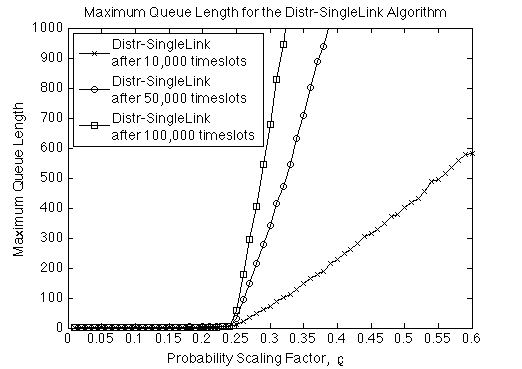
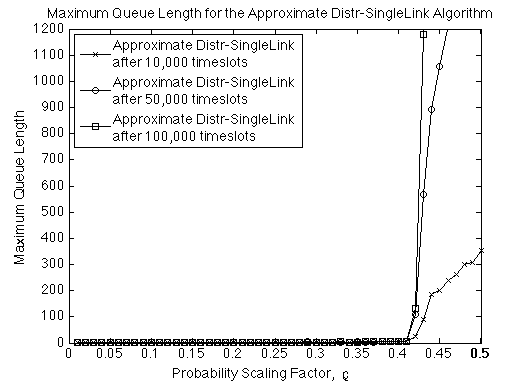
Figure 1. The maximum queue lengths for the distributed algorithm Distr-SingleLink. The problem instances are based on random topology with $n=200$, $\ell_{\min}=1$, $\ell_{\max}=20$, $\alpha=2.5$ and $\beta=1$.

We implemented General (using Distr-SingleLink) on a random topology. As Fig. 1 shows, efficiency ratios upto 0.4 is achieved, which is quite good. Details are omitted due to space restrictions.

References

- [1] Matthew Andrews and Michael Dinitz. Maximizing capacity in arbitrary wireless networks in the SINR model: Complexity and game theory. In INFOCOM, pages 1332–1340, 2009.
- [2] Eyjólfur I. Ásgeirsson, Magnús M. Halldórsson, and Pradipta Mitra. A Fully Distributed Algorithm for Throughput Performance in Wireless Networks. In CISS, 2012.
- [3] Soren Asmussen. Applied Probability and Queues. Springer, 2nd edition, 2003.
- [4] Antonis Dimakis and Jean Walrand. Sufficient conditions for stability of longest-queue-first scheduling: second-order properties using fluid limits. Advances in Applied Probabability, 38(2):505–521, 2006.
- [5] Devdatt P. Dubhashi and Alessandro Panconesi. Concentration of Measure for the Analysis of Randomized Algorithms. Cambridge University Press, 2009.
- [6] O. Goussevskaia, M. M. Halldórsson, R. Wattenhofer, and E. Welzl. Capacity of Arbitrary Wireless Networks. In INFOCOM, pages 1872–1880, April 2009.
- [7] M. M. Halldórsson and P. Mitra. Nearly optimal bounds for distributed wireless scheduling in the SINR model. In ICALP, 2011.
- [8] M. M. Halldórsson and R. Wattenhofer. Wireless Communication is in APX. In ICALP, pages 525–536, July 2009.
- [9] Magnús M. Halldórsson. Wireless scheduling with power control. In ESA, pages 361–372, 2009.
- [10] Magnús M. Halldórsson and Pradipta Mitra. Wireless Capacity with Oblivious Power in General Metrics. In SODA, 2011.
- [11] Magnus M. Halldorsson and Pradipta Mitra. Wireless capacity and admission control in cognitive radio. In INFOCOM, 2012.
- [12] Changhee Joo, Xiaojun Lin, and N.B. Shroff. Understanding the Capacity Region of the Greedy Maximal Scheduling Algorithm in Multi-Hop Wireless Networks. In INFOCOM, 2008.
- [13] T. Kesselheim. A Constant-Factor Approximation for Wireless Capacity Maximization with Power Control in the SINR Model. In SODA, 2011.
- [14] T. Kesselheim and B. Vöcking. Distributed contention resolution in wireless networks. In DISC, pages 163–178, August 2010.
- [15] Thomas Kesselheim. Dynamic packet scheduling in wireless networks. http://arxiv.org/abs/1203.1226.
- [16] Long B. Le, Eytan Modiano, Changhee Joo, and Ness B. Shroff. Longest-queue-first scheduling under SINR interference model. In MobiHoc, 2010.
- [17] Ritesh Maheshwari, Shweta Jain, and Samir R. Das. A measurement study of interference modeling and scheduling in low-power wireless networks. In SenSys, pages 141–154, 2008.
- [18] Eytan Modiano, Devavrat Shah, and Gil Zussman. Maximizing throughput in wireless networks via gossiping. In SIGMETRICS/Performance, pages 27–38, 2006.
- [19] Thomas Moscibroda, Roger Wattenhofer, and Yves Weber. Protocol Design Beyond Graph-Based Models. In Hotnets, November 2006.
- [20] Thomas Moscibroda, Roger Wattenhofer, and Aaron Zollinger. Topology control meets SINR: The scheduling complexity of arbitrary topologies. In MobiHoc, pages 310–321, 2006.
- [21] Christian Scheideler, Andréa W. Richa, and Paolo Santi. An dominating set protocol for wireless ad-hoc networks under the physical interference model. In MobiHoc, pages 91–100, 2008.
- [22] L. Tassiulas and A. Ephremides. Stability properties of constrained queueing systems and scheduling policies for maximum throughput in multihop radio networks. IEEE Trans. Automat. Contr., 37(12):1936–1948, 1992.