Interaction-induced charge and spin pumping through a quantum dot at finite bias

Abstract

We investigate charge and spin transport through an adiabatically driven, strongly interacting quantum dot weakly coupled to two metallic contacts with finite bias voltage. Within a kinetic equation approach, we identify coefficients of response to the time-dependent external driving and relate these to the concepts of charge and spin emissivities previously discussed within the time-dependent scattering matrix approach. Expressed in terms of auxiliary vector fields, the response coefficients allow for a straightforward analysis of recently predicted interaction-induced pumping under periodic modulation of the gate and bias voltage [Phys. Rev. Lett. 104, 226803 (2010)]. We perform a detailed study of this effect and the related adiabatic Coulomb blockade spectroscopy, and, in particular, extend it to spin pumping. Analytic formulas for the pumped charge and spin in the regimes of small and large driving amplitude are provided for arbitrary bias. In the absence of a magnetic field, we obtain a striking, simple relation between the pumped charge at zero bias and at bias equal to the Coulomb charging energy. At finite magnetic field, there is a possibility to have interaction-induced pure spin pumping at this finite bias value, and generally, additional features appear in the pumped charge. For large-amplitude adiabatic driving, the magnitude of both the pumped charge and spin at the various resonances saturate at values which are independent of the specific shape of the pumping cycle. Each of these values provide an independent, quantitative measurement of the junction asymmetry.

I Introduction

The generation of a dc current through a mesoscopic system is usually associated to a bias voltage maintained between the contacts to the exterior world. Remarkably, charge and spin transport can even be achieved in the absence of an external bias by the cyclic modulation of some of the parameters of the system.Thouless83 When this modulation is slow compared to the characteristic dwell time of the electrons, the transport mechanism is called adiabatic pumping. Here, the pumped charge is of geometric nature, since it depends on the specific shape of the path sustained by the system’s parameters but not on its detailed time evolution.Altshuler99 ; Avron00 ; Makhlin01 ; Zhou03 For appropriate modulation setups,Niu84 ; Avron01 the pumped charge after one period may be quantized in units of the electron charge,Kouwenhoven91 ; Pothier92 ; Chorley12 motivating its use as a highly precise current standard for quantum metrologyKeller98 or in the initialization Feve07 and processing of coherent states Beenakker05 ; Samuelsson05 ; Splettstoesser09 ; Sherkunov12 in the context of quantum information. In the opposite limit where the transferred charge is not necessarily quantized, the pumping mechanism is dominated by quantum interferenceZhou99 of the coherent electrons in the device. In the last years, adiabatic pumping was widely studied both experimentally Switkes99 ; Watson03 ; Fletcher03 and theoretically. In noninteracting systems, a well-established theory was formulated by Brouwer. Brouwer98 It makes use of the concept of emissivity which was introduced in the scattering matrix approach for time-dependent systems at low frequency by Büttiker, Thomas and Prêtre.Buttiker94 Importantly, this formalism is adequate as long as interactions can be described on a self-consistent mean-field level.Buttiker93 Within this formalism, several aspects of adiabatic pumping were explored, covering diverse effects such as dissipation and noise,Makhlin01 ; Moskalets02 or spin polarized pumping.Mucciolo02 Further works dealt with different setups including normal metal-superconducting heterostructures,Wang01 pumping by surface acoustic waves,Levinson00 and graphene-based quantum pumps.Prada09

Pumping through confined electron systems dominated by a strong Coulomb interaction is a particularly challenging topic since the mean-field approach breaks down and a new formulation is necessary. Several studies addressed interaction effects in specific setups and regimes.Citro03 ; Aono04 ; Schiller08 ; Arrachea08 ; Aleiner98 ; Brouwer05 ; Cota05 ; Splettstoesser05 ; Sela06 ; Splettstoesser06 ; Splettstoesser08 ; Cavaliere09 ; Winkler09 ; Reckermann10 ; Riwar10 ; Reckermann12 ; Kashuba12 ; Riwar12 In Ref. Citro03, , pumping is investigated in interacting quantum wires. By using a slave boson mean field approximation, Aono studied adiabatic pumping through a quantum dot in the Kondo regime.Aono04 This regime was also treated in the Toulouse limitSchiller08 and for nonadiabatic pumpsArrachea08 by using the Keldysh Green’s function technique. Pumping through open quantum dots was described by employing bosonization techniques.Aleiner98 ; Brouwer05 In the Coulomb blockade regime, spin pumping was addressed through a numerical calculation of the reduced density matrix of a double quantum dot.Cota05 An expression for the adiabatic pumping current in interacting systems was derived using a nonequilibrium Green’s function technique in Refs. Splettstoesser05, ; Sela06, . A diagrammatic real-time approach,Splettstoesser06 was used to investigate several aspects of adiabatic pumping through weakly-coupled interacting quantum-dot systemsSplettstoesser08 ; Cavaliere09 ; Winkler09 ; Reckermann10 ; Riwar10 ; Riwar12 ; Reckermann12 and served as the basis for non-equilibrium renormalization group studies that treat the tunneling non-perturbatively.Kashuba12

Among the above mentioned studies, only a few discuss the modulation of the applied bias.Moskalets04 In particular, pumping around a nonequilibrium working point induced by a static nonlinear bias was addressed in noninteracting systems.Entin-Wohlman02 Recently, a strongly interacting single-level quantum dot with a modulation of the gate and bias voltage was investigated.Reckermann10 For this modulation setup, on top of a dc current produced by the bias, an additional adiabatic dc current is generated by the Coulomb interaction. Interestingly, this interaction-induced pumping current can be accessed by using lock-in techniques, and was suggested as a new spectroscopic tool to probe internal properties of the system, like spin degeneracy and junction asymmetries. Similar effects were reportedYuge12 for an open quantum system when controlling the temperatures and chemical potentials of the reservoirs. In Ref. Riwar12, , the zero-frequency pumping noise in adiabatically driven quantum dots is discussed for time-dependent bias, revealing further information on the tunnel coupling asymmetry in cases where the pumped charge is zero.

In this paper, we investigate interaction-induced charge pumping in detail and extend it to the spin degree of freedom. We focus on the interplay between the strong local Coulomb interaction in a quantum dot and the nonequilibrium effects induced by finite bias and the modulation around this working point. To describe the dynamics of the local system, the coupling to the leads and the frequency of the modulation are treated perturbatively.Splettstoesser06 In particular, we restrict ourselves to the single-electron tunneling (SET) regime.

We derive a general expression for the adiabatic charge and spin currents in response to a change in the internal occupations of the dot induced by the driving parameters. The coefficients of this response of the current are related to the emissivities to the leads,Buttiker94 establishing a connection to Brouwer’s pumping theory Brouwer98 which is applicable as long as the single-particle picture holds. Moreover, we write the pumped charge and spin as the flux generated by auxiliary vector fields in the space of the parameters. This allows us to find the general conditions under which a finite pumped charge or spin may occur, independent of details specific to the model or the pumping cycle.

We apply this strategy for the case of a modulation of the gate and bias voltage and analyze the influence of the local interaction on the generation of pumping. The recently introduced “stability diagram” for the pumped chargeReckermann10 is shown to be readily understood in terms of these vector fields and extended to pumped spin. A detailed analysis of these diagrams is provided for all the regimes of the applied bias, including analytic fitting formulas for the pumped charge and spin in the limits of weak and large driving amplitude. We find that, although not quantized, the pumped charge (and spin) for large driving amplitudes saturates at plateau values which depend on the asymmetry in the coupling to the leads and the working region of the applied voltages. At zero magnetic field, a surprising and simple relation between the pumped charge at high-bias and at zero-bias is found. It is exploited for a quantitative determination of the junction asymmetry by two single measurements. In a finite magnetic field, the spin and charge pumping are not anymore trivially connected at high-bias. In this regime, pure spin pumping occurs when the coupling to the leads is symmetric.

Our paper is organized as follows. In the next section we introduce the model and review the theoretical framework used in the calculation of the pumped charge and spin. In Sec. III, we consider the pumped charge and spin for the specific modulation of the gate and bias voltage, first concentrating on the role of the interaction and then, in Sec. III.4, we discuss the effects induced by an external magnetic field. We summarize our results in Sec. IV.

II Model and Formalism

II.1 Model

We consider a single-level quantum dot with Coulomb interaction weakly coupled to two noninteracting leads as sketched in Fig. 1. The full system, containing the dot, the left ($L$) and right ($R$) leads, and the tunneling between dot and leads, is described by the total Hamiltonian $H(t)=H_{\mathrm{dot}}(t)+H_{\mathrm{res}}(t)+H_{\mathrm{tun}}$. The quantum dot Hamiltonian is given by

$$H_{\mathrm{dot}}(t)=\sum_{\sigma}\epsilon_{\sigma}(t)\hat{n}_{\sigma}+U\hat{n}_{\uparrow}\hat{n}_{\downarrow},$$ (1)

where we denote the spin-resolved number operator by $\hat{n}_{\sigma}=d_{\sigma}^{\dagger}d_{\sigma}$ and $U$ is the Coulomb charging energy. The fermionic operator $d_{\sigma}^{\dagger}$ ($d_{\sigma}$) creates (annihilates) an electron in the dot with spin $\sigma=\uparrow,\downarrow$. The many-body eigenstates of the dot are characterized by their charge number and spin by $\ket{0}$ for an empty dot, $\ket{\sigma}=d_{\sigma}^{\dagger}\ket{0}$ for a singly occupied dot with spin $\sigma$ and $\ket{2}=d_{\downarrow}^{\dagger}d_{\uparrow}^{\dagger}\ket{0}$ for a doubly occupied dot. Their energies are then $0,\epsilon_{\sigma}$ and $\epsilon_{\uparrow}+\epsilon_{\downarrow}+U$, respectively, where $\epsilon_{\sigma}(t)=\epsilon(t)-\sigma B/2$. The level position $\epsilon(t)=-\alpha V_{g}(t)$ is capacitively modulated by the time-dependent gate voltage $V_{g}(t)$, with lever arm $\alpha<1$. Furthermore, $B$ accounts for the Zeeman splitting produced by an external magnetic field $\mathbf{B}=B\mathbf{e}_{z}$ in units $e=\hbar=k_{B}=g\mu_{B}=1$. Here we use $\sigma=\pm 1$ as a convenient notation for spin $\uparrow$ and $\downarrow$, respectively. The underlying capacitive description of the parameters $U$ and $\alpha$ is sketched in Fig. 2 and will be discussed below.

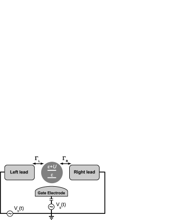
Figure 1: Scheme of the considered model. The interacting quantum dot (grey circle) is capacitively coupled to two leads via $\Gamma_{L}$ and $\Gamma_{R}$. The transport is controlled through time-dependent gate and bias voltages. The lines in the dot indicate the transition energies $\epsilon_{N}-\epsilon_{N-1}$, $N=1,2$, for zero external magnetic field $B$.

The leads are described as reservoirs of noninteracting electrons through the Hamiltonian

$$H_{\mathrm{res}}(t)=\sum_{rk\sigma}[\epsilon_{rk}+\mu_{r}(t)]c_{rk\sigma}^{\dagger}c_{rk\sigma},$$ (2)

where $c_{rk\sigma}^{{\dagger}}$ ($c_{rk\sigma}$) creates (annihilates) an electron in the lead $r=L,R$ with spin $\sigma=\uparrow,\downarrow$ and state index $k$. The eigenenergies of the leads are uniformly shifted by the time-dependent bias voltage $V_{b}(t)$ such that the electro-chemical potentials read $\mu_{r}(t)=\pm V_{b}(t)/2$ for $r=L,R$. These reservoirs are furthermore characterized by a temperature $T$.

Finally, the tunnel coupling between the dot and the leads is determined by the tunnel Hamiltonian

$$H_{\mathrm{tun}}=\sum_{rk\sigma}V_{r}d_{\sigma}^{\dagger}c_{rk\sigma}+h.c.,$$ (3)

with the tunnel matrix element $V_{r}$, which we assume to be independent of $k$ and $\sigma$. The tunnel-coupling strength $\Gamma_{r}=2\pi|V_{r}|^{2}\nu_{r}$ characterizes the rate at which tunnel processes take place. Here $\nu_{r}$ is the density of states in the $r$-lead, which is assumed to be energy-independent and with a band cutoff $D_{r}$, which is the largest energy scale.

We are interested in the simultaneous modulation of gate and bias voltages. These are driven around a time-independent working point specified by $\bar{V}_{g}$ and $\bar{V}_{b}$ with a fixed relative phase $\Delta\phi=\phi_{g}-\phi_{b}$:

$$V_{x}(t)=\bar{V}_{x}+\delta V_{x}\sin(\Omega t+\phi_{x}),\>x=g,b,$$ (4)

where $\delta V_{x}$ is the driving amplitude. At time $t_{0}$, we “switch on” the coupling between the dot and the leads and calculate the time-dependent nonequilibrium steady state at a much later time $t$. This includes two sources of nonequilibrium: the finite bias and the adiabatic driving. On top of the stationary current flow, an additional time-dependent current, which can have a dc component, is generated by the periodic modulation. We work in the adiabatic regime where the driving period $\mathcal{T}=2\pi/\Omega$ is larger than the typical time spent by the electrons inside the quantum dot. Here, the modulation frequency and the driving amplitude are limited by the adiabaticity condition $\alpha\delta V_{g},\delta V_{b}\ll T^{2}/\Omega$.

II.1.1 Observables

In the description of the dot occupancies through the reduced density matrix, we assume the reservoirs to be always in equilibrium. Since leads and dot are decoupled at the initialization time $t_{0}$, the total density matrix is factorized in both subsystems as $\hat{\rho}=\hat{p}_{\mathrm{res}}\hat{p}$, with the density matrix of the leads given by the one of a grand canonical ensemble

$$\hat{p}_{\mathrm{res}} =\prod_{r}\frac{1}{z_{r}}e^{-\left[H_{r}(t^{\prime})-\mu_{r}(t^{\prime})\hat{N}_{r}\right]/T},$$ (5a)

$$z_{r} =\operatorname*{Tr}_{r}e^{-\left[H_{r}(t^{\prime})-\mu_{r}(t^{\prime})\hat{N}_{r}\right]/T},$$ (5b)

and $t^{\prime}\leq t_{0}$. Here $\hat{N}_{r}=\sum_{k\sigma}c_{rk\sigma}^{\dagger}c_{rk\sigma}$ is the particle-number operator in the $r$-lead and the temperature $T$ is assumed to be the same in the two leads. Notice that the density operator of the reservoirs remains time-independent, meaning that the occupation in the leads is not affected by the modulation of the bias voltage. For electric field modulations with a frequency well below the plasma frequency of the leads (tens of $\mathrm{THz}$ in typical doped semiconductors) this assumption is well justified.Jauho94

The time evolution of the expectation value of an arbitrary operator $\hat{R}$ is formally obtained by

$$R(t)=\braket{\hat{R}}(t)=\operatorname*{Tr}_{\mathrm{dot}}\operatorname*{Tr}_{\mathrm{res}}\left(\hat{R}\,\hat{\rho}(t)\right).$$ (6)

In the next sections, we will describe the tunneling currents $I_{r}(t)=\braket{\hat{I}_{r}}(t)$ and $J_{r}(t)=\braket{\hat{J}_{r}}(t)$ related to the charge and the spin component along the external field $B$, respectively, entering the $r$-lead. Since in the uncoupled system $H_{0}=H_{\mathrm{dot}}+H_{\mathrm{res}}$ the number of particles and the $z$-component of spin are conserved, the operators related to these observables are given by

$$\hat{I}_{r} =i[H_{\mathrm{tun}},\hat{N}_{r}],$$ (7a)

$$\hat{J}_{r} =i[H_{\mathrm{tun}},\hat{S}_{z}^{r}],$$ (7b)

with $\hat{S}_{z}^{r}=\sum_{k\sigma}\frac{\sigma}{2}c_{rk\sigma}^{\dagger}c_{rk\sigma}$. Since we consider a system that preserves rotation symmetry around the magnetic field ($z$-) axis, the $x$ and $y$ components of the spin vector may only occur as a transient effect and are not required here.

II.2 Real-time diagrammatic approach

In this section we outline the theoretical framework used to identify the adiabatic contribution to the time-resolved currents of Eq. (6). As we will show in Eqs. (14) and (15), the adiabatic current can be interpreted as the delayed response of the dot occupation probabilities to the driving of the external parameters. The full relevance of this result will become clear in the next section. Eq. (15) allows to apply the concept of emissivity to a system with strong Coulomb interaction and arbitrary bias. Originally,Buttiker94 the emissivity was introduced to describe capacitive effects on time-dependent response on a self-consistent mean-field level and was further used on adiabatic pumping through non- or weakly interacting systems. Brouwer98 ; Sela06

We start with the description of the relevant part of the dot’s reduced density matrix, namely, its diagonal elements, obtained after tracing out the degrees of freedom of the leads. The time evolution of the dot occupation probabilities, represented by the vector $\mathbf{p}(t)=(p_{0}(t),p_{\uparrow}(t),p_{\downarrow}(t),p_{2}(t))^{\mathrm{T}}$, is governed by the generalized master equationSplettstoesser06

$$\frac{d}{dt}\mathbf{p}(t)=\int_{-\infty}^{t}dt^{\prime}\mathbf{W}(t,t^{\prime})\mathbf{p}(t^{\prime}).$$ (8)

Here, the change in the dot occupation probabilities, due to electron tunnel processes between dot and leads, is accounted by the kernel $\mathbf{W}(t,t^{\prime})$. In terms of the real-time diagrammatic technique developed in Ref. Konig96, , this kernel collects all irreducible diagrams in the Keldysh double contour. Its matrix elements $W_{m,n}(t,t^{\prime})$ describe the transition from a state $\ket{n}$ at time $t^{\prime}$ to a state $\ket{m}$ at time $t$. It is important to notice that the transport properties are completely determined by the diagonal elements of the reduced density operator. In the chosen basis the off-diagonal elements, related to coherent superposition of different states, are decoupled from diagonal ones due to charge and spin conservation in the tunneling and therefore do not affect the currents.

Since we consider a weakly coupled system bounded to a slow modulation of the energy levels, it is sufficient to describe the lowest order contribution in the tunnel coupling and in the time-dependent perturbation introduced by the driving. The occupation probabilities are thus expanded in powers of $\Omega$ by $\mathbf{p}(t)=\mathbf{p}_{t}^{(i)}+\mathbf{p}_{t}^{(a)}$, bearing in mind that $\Omega/\Gamma\ll 1$. The first term (zeroth-order in $\Omega$) represents the instantaneous occupations and describes the steady state solution when the parameters are frozen at time $t$. Here the index $t$ indicates the parametric time-dependence through the driving parameters $\{\chi(t)\}$, i.e. $\mathbf{p}_{t}^{(i)}=\mathbf{p}^{(i)}(\{\chi(t)\})$. The instantaneous occupations are obtained from the time-dependent kinetic equation in the stationary limit

$$\mathbf{0}=\mathbf{W}_{t}^{(i)}\mathbf{p}_{t}^{(i)},$$ (9)

together with the normalization condition $\mathbf{e}^{\mathrm{T}}\mathbf{p}_{t}^{(i)}=1$, where $\mathbf{e}=(1,1,1,1)^{\mathrm{T}}$, and we introduced the zero-frequency Laplace transform of the instantaneous kernel $\mathbf{W}_{t}^{(i)}=\int_{-\infty}^{t}dt^{\prime}\mathbf{W}^{(i)}(t-t^{\prime})$. In the SET regime we consider here, characterized by the linear dependence on $\Gamma$ of $\mathbf{W}_{t}^{(i)}$, the result coincides with the one from Fermi’s golden rule. The next-to-leading term (linear in $\Omega$), $\mathbf{p}_{t}^{(a)}$, obeys the adiabatic correction to the kinetic equation

$$\frac{d}{dt}\mathbf{p}_{t}^{(i)}=\mathbf{W}_{t}^{(i)}\mathbf{p}_{t}^{(a)}.$$ (10)

The retardation correction $\mathbf{p}_{t}^{(a)}$ is determined by the competition between the driving (left hand side) and the inverse response times contained in $\mathbf{W}_{t}^{(i)}$ (right hand side). The dot occupation probabilities are obtained by solving Eqs. (9) and (10) together with the normalization condition $\mathbf{e}^{\mathrm{T}}\mathbf{p}_{t}^{(i)}=1$ and $\mathbf{e}^{\mathrm{T}}\mathbf{p}_{t}^{(a)}=0$. From Eq. (10), the adiabatic corrections to the occupation probabilities are written in terms of the instantaneous contributions by

$$\mathbf{p}_{t}^{(a)}=\left[\tilde{\mathbf{W}}_{t}^{(i)}\right]^{-1}\frac{d}{dt}\mathbf{p}_{t}^{(i)},$$ (11)

where the (invertible) matrix

$$\left[\tilde{\mathbf{W}}_{t}^{(i)}\right]_{ij}=\left[\mathbf{W}_{t}^{(i)}\right]_{ij}-\left[\mathbf{W}_{t}^{(i)}\right]_{ii},$$ (12)

includes the normalization condition $\mathbf{e}^{\mathrm{T}}\mathbf{p}_{t}^{(a)}=0$.

The charge and spin currents in Eq. (6) need to be equally expanded in both the frequency $\Omega$ and the tunnel-coupling strength $\Gamma$. The resulting observables are then split into instantaneous and adiabatic correction terms

$$R_{t}^{(i/a)}=\braket{\hat{R}}_{t}^{(i/a)}=\mathbf{e}^{\mathrm{T}}\mathbf{W}_{R,t}^{(i)}\mathbf{p}_{t}^{(i/a)},$$ (13)

where $\mathbf{W}_{R,t}^{(i)}$ is the instantaneous kernel of the corresponding current $R$ which, in the present approximation, is linear in $\Gamma$. We describe $R_{t}^{(a)}$ by a scalar product with the time-derivative of the dot state occupation probabilities

$$R_{t}^{(a)} =\mathbf{e}^{\mathrm{T}}\mathbf{W}_{R,t}^{(i)}\left[\tilde{\mathbf{W}}_{t}^{(i)}\right]^{-1}\frac{d}{dt}\mathbf{p}_{t}^{(i)}$$ (14a)

$$:=\left[\boldsymbol{\varphi}_{t}^{R}\right]^{\mathrm{T}}\frac{d}{dt}\mathbf{p}_{t}^{(i)}$$ (14b)

$$=\sum_{j}\varphi_{j,t}^{R}\frac{d}{dt}p_{j,t}^{(i)},$$ (14c)

with the sum running over the dot eigenstates, i.e. $j=0,\uparrow,\downarrow,2$. Applied to the adiabatic charge and spin currents, this equation defines the adiabatic current $R$ as the response to a time-dependent variation in the instantaneous occupation probabilities induced by the external modulation. The response coefficient,

$$\varphi_{j,t}^{R}=\frac{\partial R_{t}^{(a)}}{\partial\dot{p}_{j,t}^{(i)}},$$ (15)

determines the ratio at which the current $R$ flows into the $r$-lead due to a variation in the occupation of the state $j$. The relevance of these coefficients lies in the fact that they distinguish the amount of charge (or spin) that enters into each one of the leads. As compared to the instantaneous solution, the response coefficients give information about the characteristic delay time for the current $R$.Kashuba12

II.3 Adiabatically pumped charge and spin

Now that we have an explicit expression for the adiabatic current, we can determine the charge and spin pumped through the quantum dot during one modulation cycle. The purpose of this section is to relate the resulting pumped charge and spin to the emissivity of the contacts,Buttiker94 a well-known concept from scattering theory. It measures the amount of charge entering the $r$-lead due to the variation $\delta\chi$ of the driving parameter $\chi$. Following the reasoning by Büttiker et al,Buttiker94 for a slow variation of $\chi$, the charge entering the $r$-lead is related to the emissivity $dN(r)/d\chi$ by

$$\delta Q_{I_{r}}=\frac{dN(r)}{d\chi}\delta\chi.$$ (16)

We are interested in the adiabaticnote1 pumped charge when varying two parameters $\chi_{1}(t)$ and $\chi_{2}(t)$ over a cycle of the driving. Calculated as the integral of Eq. (16), this readsBrouwer98

$$Q_{I_{r}}=\int_{0}^{\mathcal{T}}dt\left(\frac{dN(r)}{d\chi_{1}}\frac{d\chi_{1}}{dt}+\frac{dN(r)}{d\chi_{2}}\frac{d\chi_{2}}{dt}\right).$$ (17)

In terms of the adiabatic current of Eq. (14), this last can also be written as

$$Q_{I_{r}} =\int_{0}^{\mathcal{T}}dtI_{r,t}^{(a)}$$ (18a)

$$=\sum_{j}\int_{0}^{\mathcal{T}}dt\,\varphi_{j,t}^{I_{r}}\frac{d}{dt}p_{j,t}^{(i)}.$$ (18b)

Since $p_{j,t}^{(i)}$ depends on $t$ through the driving parameters, we rewrite its time-derivative in terms of $\dot{\chi}_{1,2}$. A comparison with Eq. (17) allows one to relate the emissivity with the response coefficients and the occupation probabilities by

$$\frac{dN(r)}{d\chi}=\sum_{j}\varphi_{j}^{I_{r}}\frac{\partial p_{j}^{(i)}}{\partial\chi},$$ (19)

where $\chi$ is either $\chi_{1}$ or $\chi_{2}$ and the index $t$ is removed to emphasize that $\varphi_{j}^{I_{r}}$ and $p_{j}^{(i)}$ are functions of $\chi$ rather than $t$. Analogously, the above relation can also be generalized for the spin emissivityBrataas12 $dS(r)/d\chi$ in terms of the spin current response coefficients as follows

$$\frac{dS(r)}{d\chi}=\sum_{j}\varphi_{j}^{J_{r}}\frac{\partial p_{j}^{(i)}}{\partial\chi}.$$ (20)

Written in this way, the emissivity is the weighted rate of change in the occupation probabilities due to the external perturbation. The response coefficients $\varphi_{j}^{I_{r}}$ and $\varphi_{j}^{J_{r}}$ describe the rate at which the charge and the spin, respectively, are transferred to the leads when the occupation probabilities are changed by the driving parameters. The above Eqs. (19) and (20), also shown by Sela and OregSela06 for adiabatic transport at equilibrium, extend the known result from scattering matrix theory Buttiker94 ; Brouwer98 to a system with strong Coulomb interaction driven around a nonequilibrium steady state.

II.3.1 Pseudo vector potential and pseudo magnetic field

We now describe the pumped charge and spin in terms of auxiliary vector fields defined in the space of the driving parameters. Our purpose here is to relate these vector fields with the response coefficients of Eq. (15). As we will show in the next section, using these fields we can conveniently describe the conditions for finite pumping and provide a detailed insight into the “stability diagrams” for the pumped charge and spin.

According to Eqs. (17) and (18), the charge and spin pumped in a cycle of the modulation can be written as the line integral

$$Q_{R}=\oint_{C}d\boldsymbol{\chi}\cdot\mathbfcal{A}_{R}(\boldsymbol{\chi}).$$ (21)

For the two-dimensional parameter space studied here, spanned by $\mathbf{e}_{\chi_{1}}=(1,0)$ and $\mathbf{e}_{\chi_{2}}=(0,1)$, the position in the closed trajectory $C$ is indicated by $\boldsymbol{\chi}=\sum_{i}\chi_{i}\mathbf{e}_{i}$. This integral is independent of how fast the path is traversed, and consequently the total pumped charge (or spin) does not depend on the driving frequency as long as the adiabaticity condition is fulfilled. The geometric aspects of the problem, entering through the field $\mathbfcal{A}_{R}$, are certainly of interest. Avron00 ; Zhou03 ; Cohen03 However, here they are merely convenient auxiliary quantities to analyze the problem of interaction-induced pumping. In analogy to classical electrodynamics, the vector field

$$\mathbfcal{A}_{R}(\boldsymbol{\chi})=\sum_{j}\varphi_{j}^{R}(\boldsymbol{\chi})\boldsymbol{\nabla}p_{j}^{(i)}(\boldsymbol{\chi}),$$ (22)

with $\boldsymbol{\nabla}=\sum_{i}\partial_{\chi_{i}}\mathbf{e}_{i}$, can be interpreted as a pseudo vector potential defined in the space of the driving parameters. From Eqs. (19) and (20), the components of this vector potential are given by the emissivities to the leads, i.e. $\mathbfcal{A}_{I_{r}}=dN(r)/d\boldsymbol{\chi}$ and $\mathbfcal{A}_{J_{r}}=dS(r)/d\boldsymbol{\chi}$. Therefore, the vector potentials describe, respectively, the amount of charge and spin entering the leads due to the change in the driving parameters. From the form of $\mathbfcal{A}_{R}$ in Eq. (22), we notice that for constant response coefficients, the resulting pseudo vector potential is just a gauge function $\mathbfcal{A}_{R}=\sum_{j}\boldsymbol{\nabla}(\varphi_{j}^{R}p_{j}^{(i)})$ which, integrated over a closed trajectory, gives zero pumping.

Using Stokes’ theorem we write the pumped charge and spin in terms of the surface integral

$$Q_{R}=\iint_{\Sigma}d\mathbf{S}\cdot\mathbfcal{B}_{R}(\boldsymbol{\chi}),$$ (23)

where $\Sigma$ is any area in the parameter space encircled by $C$, such that $C=\partial\Sigma$. Written in this way, we can imagine the pumped charge and spin as the flux generated by a pseudo magnetic field

$$\mathbfcal{B}_{R}(\boldsymbol{\chi}) =\boldsymbol{\nabla}\times\mathbfcal{A}_{R}(\boldsymbol{\chi})$$ (24a)

$$=\sum_{j}\boldsymbol{\nabla}\varphi_{j}^{R}(\boldsymbol{\chi})\times\boldsymbol{\nabla}p_{j}^{(i)}(\boldsymbol{\chi}).$$ (24b)

The advantage of this representation is that the pseudo magnetic field anticipates the conditions for finite pumping without referring to the specific details of the model and the modulation. The direction of this field is, by construction, perpendicular to the plane (i.e. pointing outside the parameter space) defined by the driving parameters, i.e. $\mathbfcal{B}_{R}(\boldsymbol{\chi})=\mathcal{B}_{R}(\boldsymbol{\chi})\,\mathbf{e}_{\chi_{1}}\times\mathbf{e}_{\chi_{2}}$. For a fixed direction of the driving, the sign of the pumped charge is given by the sign of $\mathcal{B}_{R}$, which depends on the internal details of the system (e.g., Coulomb interaction, coupling to the leads, spin degeneracy). We stress that this interpretation of $Q_{R}$ comes purely from the adiabaticity condition in the time-dependent parameters, and should not be confused with any other effect due to the external magnetic field $B$ eventually present in this setup.

III Results

In this section, we apply the above theory for the specific case of a single-level quantum dot slowly driven by the gate and bias voltage. In particular, we want to understand how the pumped charge and spin are affected by the interplay between the local Coulomb interaction and nonequilibrium effects induced by a modulation around a finite bias. To this end, we introduce expressions for the adiabatic charge and spin currents for a general modulation and then we take the specific modulation of the voltages given in Eq. (4).

Our starting point is the description of the time-resolved adiabatic charge current given in Eq. (14). This is obtained from the explicit calculation of the matrix elements of the kernels $\mathbf{W}_{t}^{(i)}$ and $\mathbf{W}_{I_{r},t}^{(i)}$ introduced in the previous section. In the evaluation of the response coefficients related to the occupation of the different states of the dot [see Eq. (15)], we find out that it is possible to combine them in such a way that the adiabatic current can be written in terms of the time-derivatives of the instantaneous average charge $\braket{\hat{n}}_{t}^{(i)}=p_{\uparrow,t}^{(i)}+p_{\downarrow,t}^{(i)}+2p_{2,t}^{(i)}$ and spin $\braket{\hat{S}_{z}}_{t}^{(i)}=(p_{\uparrow,t}^{(i)}-p_{\downarrow,t}^{(i)})/2$. We recover the result Reckermann10

$$I_{r,t}^{(a)}=\varphi_{n,t}^{I_{r}}\frac{d}{dt}\braket{\hat{n}}_{t}^{(i)}+\varphi_{S_{z},t}^{I_{r}}\frac{d}{dt}\braket{\hat{S}_{z}}_{t}^{(i)},$$ (25)

where the charge current response coefficients, related to the charge and spin in the dot, respectively, read

$$\varphi_{n,t}^{I_{r}} =-\frac{(\Gamma-\gamma)(\Gamma_{r}+\gamma_{r})+\beta\beta_{r}}{\Gamma^{2}-\gamma^{2}+\beta^{2}},$$ (26a)

$$\varphi_{S_{z},t}^{I_{r}} =-2\frac{(\Gamma_{r}+\gamma_{r})\beta-(\Gamma+\gamma)\beta_{r}}{\Gamma^{2}-\gamma^{2}+\beta^{2}}.$$ (26b)

together with $\gamma=\sum_{r}\gamma_{r}$, $\beta=\sum_{r}\beta_{r}$, and $\Gamma=\sum_{r}\Gamma_{r}$. The response coefficients depend parametrically on $t$ through the following factors

$$\gamma_{r} =\frac{\Gamma_{r}}{2}\sum_{\sigma}\left[f\left(\frac{\epsilon_{r\sigma}}{T}\right)-f\left(\frac{\epsilon_{r\sigma}+U}{T}\right)\right],$$ (27a)

$$\beta_{r} =\frac{\Gamma_{r}}{2}\sum_{\sigma}\sigma\left[f\left(\frac{\epsilon_{r\sigma}}{T}\right)-f\left(\frac{\epsilon_{r\sigma}+U}{T}\right)\right].$$ (27b)

Since the adiabatic charge currents flowing into each one of the leads are related by particle conservation, i.e. $\sum_{r}I_{r,t}^{(a)}=-\frac{d}{dt}\braket{\hat{n}}_{t}^{(i)}$, no net charge is accumulated on the dot after one period of the modulation.

Noticeably, the above expression for the adiabatic charge current is not restricted to a particular choice of the driving parameters. In this sense, Eq. (25) is valid for arbitrary combinations involving not only the voltages $V_{g}(t)$ and $V_{b}(t)$ but also $\Gamma_{r}(t)$, $B(t)$ (in a fixed direction), $U(t)$, etc., because the eigenstates of the system remain time-independent. For the specific modulation we consider here, given by Eq. (4), the time dependence exclusively enters in the arguments

$$\epsilon_{r\sigma}(t)=\epsilon_{\sigma}(t)-\mu_{r}(t),$$ (28)

of the Fermi function $f(\omega)=[1+\exp(\omega)]^{-1}$. We now extend the above calculation for the adiabatic spin current. From the evaluation of the matrix elements of $\mathbf{W}_{J_{r},t}^{(i)}$ we obtain

$$J_{r,t}^{(a)}=\varphi_{n,t}^{J_{r}}\frac{d}{dt}\braket{\hat{n}}_{t}^{(i)}+\varphi_{S_{z},t}^{J_{r}}\frac{d}{dt}\braket{\hat{S}_{z}}_{t}^{(i)}.$$ (29)

In this case, the spin current response coefficients are

$$\varphi_{n,t}^{J_{r}} =-\frac{1}{2}\frac{(\Gamma-\gamma)\beta_{r}-(\Gamma_{r}-\gamma_{r})\beta}{\Gamma^{2}-\gamma^{2}+\beta^{2}},$$ (30a)

$$\varphi_{S_{z},t}^{J_{r}} =-\frac{(\Gamma+\gamma)(\Gamma_{r}-\gamma_{r})+\beta_{r}\beta}{\Gamma^{2}-\gamma^{2}+\beta^{2}}.$$ (30b)

For the spin-isotropic quantum dot discussed here, the adiabatic spin current only occurs in the presence of an external magnetic field. For $B=0$ at any time, rotation symmetry implies $\braket{S_{z}}_{t}^{(i)}=0$ and $\beta_{r}=0$, such that the current vanishes for all times. The spin currents $J_{L,t}^{(a)}$ and $J_{R,t}^{(a)}$ are related by spin conservation, i.e. $\sum_{r}J_{r,t}^{(a)}=-\frac{d}{dt}\braket{\hat{S_{z}}}_{t}^{(i)}$, meaning that no accumulation of spin is allowed after one cycle of the parameter modulation.

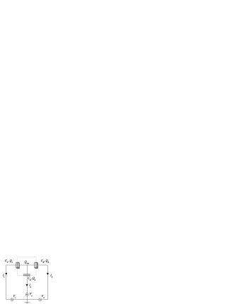
Figure 2: Schematics of the equivalent circuit for the proposed model. $C_{L},C_{R}$ are the capacitances between the dot and the leads and $C_{g}$ is the capacitance between the dot and the gate electrode. The quantum dot region is indicated by dashed lines.

III.1 Displacement current and pseudo gauge invariance

In addition to the tunneling currents we introduced above, a displacement current:

$$I_{r}^{\mathrm{dis}}(t)=\frac{d}{dt}Q_{r}^{\mathrm{scr}}(t),$$ (31)

generally occurs in the present setup due to the moving screening charges $Q_{r}^{\mathrm{scr}}$ in the gate and the leads. These arise in response to a variation in the electrostatic potential induced by a change of the charge on the dot. To describe them, we consider the Coulomb-blockade model,Averin91 in which the system is represented by the equivalent circuit shown in Fig. 2. The screening charges are given by the difference

$$Q_{r}^{\mathrm{scr}}(t)=C_{r}\left[V_{r}(t)-V_{\mathrm{dot}}(Q_{\mathrm{dot}}(t))\right],$$ (32)

between the applied voltage at the $r$-lead and the electrostatic potential inside the dot (in Fig. 2, the region delimited by dashed lines). $C_{r}$ is the capacitance between the dot and the $r$-lead. Due to particle conservation we have $\dot{Q}_{\mathrm{dot}}(t)=d\braket{\hat{n}}/dt=-[I_{L}(t)+I_{R}(t)]$ and the displacement current readsBruder94

$$I_{r}^{\mathrm{dis}}(t)=C_{r}\dot{V}_{r}(t)-\frac{C_{r}}{C}\sum_{r^{\prime}}\left[C_{r^{\prime}}\dot{V}_{r^{\prime}}(t)+I_{r^{\prime}}(t)\right],$$ (33)

where $C=C_{L}+C_{R}+C_{g}$ is the total capacitance. As in the case of the tunneling currents, we can separate the displacement current into instantaneous and adiabatic contributions. Since the time-derivatives of the applied voltages are of linear order in $\Omega$, they do not enter in the instantaneous term and

$$I_{r,t}^{\mathrm{dis},(i)}=-\frac{C_{r}}{C}\sum_{r^{\prime}}I_{r^{\prime},t}^{(i)}.$$ (34)

However, since $I_{r,t}^{(i)}$ corresponds to the instantaneous steady-state solution [see Eqs. (9) and (13)], particle conservation implies $I_{L,t}^{(i)}+I_{R,t}^{(i)}=0$ and therefore $I_{r,t}^{\mathrm{dis},(i)}$ is exactly zero for any value of $t$, as required. For the adiabatic correction to the displacement current we have

$$I_{r}^{\mathrm{dis},(a)}=C_{r}\dot{V}_{r}(t)-\frac{C_{r}}{C}\sum_{r^{\prime}}C_{r^{\prime}}\left[\dot{V}_{r^{\prime}}(t)+I_{r^{\prime},t}^{(a)}\right].$$ (35)

Here one notices that although this current can have finite values during the driving cycle, its time-average over one period is zero. This becomes evident since particle conservation yields $I_{L,t}^{(a)}+I_{R,t}^{(a)}=-\frac{d}{dt}\braket{\hat{n}}_{t}^{(i)}$ such that the above is a total time-derivative.

In terms of the vector fields of the previous section, the displacement current is related to an irrotational pseudo vector potential

$$\mathbfcal{A}_{I_{r}^{\mathrm{dis}}}=C_{r}\boldsymbol{\nabla}V_{r}-\frac{C_{r}}{C}\sum_{r^{\prime}}C_{r^{\prime}}\boldsymbol{\nabla}V_{r^{\prime}}+\frac{C_{r}}{C}\boldsymbol{\nabla}\braket{\hat{n}}^{(i)},$$ (36)

which can be imagined as a gauge function, $\mathbfcal{A}_{I_{r}^{\mathrm{dis}}}=\boldsymbol{\nabla}\psi$, that leaves the total pseudo magnetic field unchanged, i.e. $\mathbfcal{B}_{I_{r}^{\mathrm{tot}}}=\boldsymbol{\nabla}\times(\mathbfcal{A}_{I_{r}}+\boldsymbol{\nabla}\psi)=\boldsymbol{\nabla}\times\mathbfcal{A}_{I_{r}}$. Since the pumped charge is due to this pseudo magnetic field, we can focus in what follows only on tunneling currents.

Now that we have the formal expressions for the adiabatic charge and spin currents, we can start with the analysis of the pumping for the specific modulation of the gate and bias voltage [see Eq. (4)] and fix the direction of the driving by taking $\phi_{g}=-\pi/2$ and $\phi_{b}=\pi$ for which the adiabatic dc current is maximal. Motivated by a previous study on interaction-induced pumping, Reckermann10 we describe in the following sections the pumping of charge and spin making use of the vector fields of Eqs. (22) and (24). Since we are interested in the effect of the interaction $U$ on the pumping, we first consider the case $U=0$ as a reference. We then analyze the role of the local interaction $U>0$ for $B=0$ and characterize the mechanism of pumping. Finally, in Sec. III.4, we extend the description of the pumped charge and introduce the pumped spin by including an external magnetic field $B>0$.

III.2 Non-interacting quantum dot

For $U=0,B\geq 0$ we observe that the charge current response coefficients [see Eq. (26)] are time-independent since $\gamma_{r}=\beta_{r}=0$. Therefore, the adiabatic response is unaffected by the change in the dot occupation during the full cycle. This means that the same amount of charge that flows into the dot from the $r$-lead during the loading part of the cycle, characterized by $d\braket{\hat{n}}_{t}^{(i)}/dt>0$, is returned to the same lead during the unloading. This constitutes a clear example in which the loading/unloading symmetry is preserved after a complete cycle of the driving. The analysis is also valid for the adiabatic spin current, where the loading/unloading symmetry is manifested through the average spin inside the dot. Therefore, although there is a finite charge and spin current

$$I_{r,t}^{(a)} =-\frac{\Gamma_{r}}{\Gamma}\frac{d}{dt}\braket{\hat{n}}_{t}^{(i)},$$ (37a)

$$J_{r,t}^{(a)} =-\frac{\Gamma_{r}}{\Gamma}\frac{d}{dt}\braket{\hat{S}_{z}}_{t}^{(i)},$$ (37b)

the total pumped charge and spin, obtained after integrating over the full period, are exactly zero. In terms of the vector field introduced in Eq. (22), the constant response is then described as an irrotational vector potential $\mathbfcal{A}_{R}=\boldsymbol{\nabla}\left[\varphi_{n}^{R}\braket{\hat{n}}^{(i)}+\varphi_{S_{z}}^{R}\braket{\hat{S}_{z}}^{(i)}\right]$, with $R$ either $I_{r}$ or $J_{r}$, whose corresponding pseudo magnetic field $\mathbfcal{B}_{R}=\boldsymbol{\nabla}\times\mathbfcal{A}_{R}$ is indeed zero. We emphasize that this result depends on the particular choice of the driving parameters. Other setups involving time-dependent barriers yield finite pumping even in the $U=0$ limit since the response coefficients are time-dependent and the loading/unloading symmetry is not necessarily preserved.Splettstoesser06

III.3 Interacting quantum dot at zero magnetic field

We now focus on the effect of a finite Coulomb interaction $U\gg T>\Gamma$ by considering $B=0$. Once the mechanism that generates the pumping is understood, we extend, in Sec. III.4, the discussion to a finite magnetic field.

In Fig. 3 we show the pseudo magnetic field of Eq. (24) in terms of the driving parameters $V_{g}$ and $V_{b}$ (from hereon called ‘stability diagram for the pseudo magnetic field for the pumped charge’). This map is a convenient tool in the characterization of the pumped charge (and later on the pumped spin) for different regimes of the applied bias and arbitrary asymmetry in the coupling to the leads. In this example, we show the pseudo magnetic field $\mathcal{B}_{I_{L}}$ related to the adiabatic charge current entering the left lead. As observed in Ref. Reckermann10, , it displays four peaks of linear dimension $\sim T$, located in the vicinity of the meeting point of two resonance lines of the differential conductance, namely, at the corner points of the regions of stable charge in the quantum dot. These lines can be approximated by the dot-level resonance conditions $\mu_{r}=\epsilon,\epsilon+U$, respectively, with $\epsilon=-\alpha V_{g}$ and $r=L,R$ (grey dashed lines in the figure). The low-bias peaks [labeled by (1) and (3) in Fig. 3] are dominant, while the high-bias peaks [(2) and (4)], emerge only when we include an asymmetry $\lambda=(\Gamma_{L}-\Gamma_{R})/\Gamma$ between the two barriers. We first investigate the regions in which $\mathcal{B}_{I_{L}}$ is zero and then we separate the discussion of the peaks according to the applied bias around which the driving takes place.

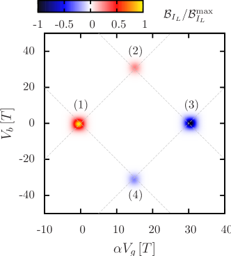
Figure 3: (Color online) Stability diagram for the pumped charge: normalized pseudo magnetic field as function of the driving parameters $V_{g}$ and $V_{b}$, for $B=0$. Grey dashed lines correspond to dot level resonance lines. The chosen Coulomb interaction and junction asymmetry are, respectively, $U=30T$ and $\lambda=0.25$.

Since we consider $B=0$, the singly occupied dot states are degenerate, i.e. $\epsilon_{r\sigma}=\epsilon-\mu_{r}$ for $\sigma=\uparrow,\downarrow$, such that $\braket{\hat{S}_{z}}_{t}^{(i)}=0$ and the adiabatic spin current completely vanishes. In this case, the adiabatic charge current reduces to

$$I_{r,t}^{(a)} =-\frac{\Gamma_{r}+\gamma_{r}}{\Gamma+\gamma}\frac{d}{dt}\braket{\hat{n}}_{t}^{(i)},$$ (38a)

$$\braket{\hat{n}}_{t}^{(i)} =2\frac{\sum_{r}\Gamma_{r}f(\epsilon_{r}/T)}{\Gamma+\gamma},$$ (38b)

and admits the following interpretation: As soon as the driving passes through a resonance line, the occupation in the quantum dot is changed and generates a response current flowing from/into the leads. The contribution flowing through the $r$-barrier is then given by the ratio $(\Gamma_{r}+\gamma_{r})/(\Gamma+\gamma)$ between the charge relaxation rate relative to the $r$-lead, i.e. $\Gamma_{r}+\gamma_{r}$, and the total relaxation rate $\Gamma+\gamma$ corresponding to the sum of the two leads. When taking the time-average over a complete cycle, the occurrence of a dc component of the adiabatic current is tied to an asymmetry between the loading and unloading parts of the cycle. We can find two regimes in which this condition is not fulfilled: (i) When the driving is far away from any resonance line, the occupation in the dot remains constant and the response is exactly zero. (ii) When the driving crosses a single resonance line, the response is symmetric during the loading and unloading. Therefore, the same amount of charge that enters the dot from the $r$-lead during the loading returns to the same lead in the unloading, such that the dc component of the adiabatic current is zero. In terms of the pseudo magnetic field

$$\mathbfcal{B}_{I_{r}}=\boldsymbol{\nabla}\varphi_{n}^{I_{r}}\times\boldsymbol{\nabla}\braket{\hat{n}}^{(i)},$$ (39)

we observe that far away from any resonance line, the gradient of the average charge is exponentially suppressed. On the other hand, when the trajectory $\partial\Sigma$ traced by the driving parameters only crosses a single resonance line, the response coefficient $\varphi_{n}^{I_{r}}$ and the average charge $\braket{\hat{n}}^{(i)}$ depend on the same effective parameter and the vectors in Eq. (39) become parallel to each other. In this sense, adiabatic transport along a single resonance line can be understood as single parameter pumping, Kohler05 which is well known to give zero contribution to the time-averaged current in the adiabatic limit.Brouwer98

In the remainder of this section, we analyze the discrete points around which the pseudo magnetic field is nonzero and calculate the 2D resonance shape of the related pumped charge. To this end, we first notice that for the modulation we consider in Eq. (4), it is convenient to write the driving parameters as they enter in the arguments of the Fermi function, i.e.

$$\chi_{r}(t)=-\frac{\alpha V_{g}(t)}{T}\mp\frac{V_{b}(t)}{2T},$$ (40)

for $r=L,R$, respectively. Motivated by the location of the peaks in the pseudo magnetic field, we investigate first the pumping at low bias, characterized by the peaks marked by (1) and (3) in Fig. 3 and then we consider the high-bias peaks (2) and (4). Once we know the behavior of these peaks, a complete description of the stability diagram for the pumped charge can be obtained from the symmetries of $\mathcal{B}_{I_{r}}$ with respect to a reflection of the applied voltages (see Appendix A).

III.3.1 Low-bias regime

We now calculate the pseudo magnetic field for the low-bias peak (1) around the point $(\alpha V_{g},V_{b})=(0,0)$. In this case, we take the gradient of the response coefficient and the average charge in Eq. (39) with respect to the driving parameters of Eq. (40) and obtain

$$\mathcal{B}_{I_{L}}^{(0,0)}(\boldsymbol{\chi})\simeq\frac{\Gamma}{8(\Gamma+\gamma)^{3}}\frac{\Gamma_{L}\Gamma_{R}}{\cosh^{2}\left(\frac{\chi_{L}}{2}\right)\cosh^{2}\left(\frac{\chi_{R}}{2}\right)},$$ (41)

with $\gamma\simeq\sum_{r}\Gamma_{r}f(\chi_{r})$ and $\boldsymbol{\chi}=(\chi_{L},\chi_{R})$. The superscript in $\mathcal{B}_{I_{L}}$ labels the origin of coordinates with respect to which $\chi_{L}$ and $\chi_{R}$ is measured. Notice here that the sign of the field is independent of the coupling asymmetry $\lambda$. In particular, for the chosen direction of the pumping cycle, the positive sign indicates that the response current through the left lead is stronger during the unloading part of the cycle. Additionally, the pseudo magnetic field decays exponentially for $\chi\gg 1$, which, as we will show later, implies an asymptotic value for the pumped charge when the enclosed area is larger than the typical support of the field ($\sim 5T$).

Now that we know the specific shape of $\mathcal{B}_{I_{L}}$, we can determine the condition at which the pumped charge is maximal, i.e. we need to know the position $(\chi_{L},\chi_{R})$ where the pseudo magnetic field reaches its maximum value. The exact position is obtained from the roots of a quartic equation (see Appendix B), which can be approximated through the interpolation between the maximum points for $\lambda=0$ and $\lambda=\pm 1$, i.e.

$$\chi_{L,R}\simeq\ln(1+\sqrt{3})\lambda\frac{\lambda\pm 1}{2}+\ln\left(\frac{1+\sqrt{33}}{4}\right)(1-\lambda^{2}).$$ (42)

In Fig. 4 we show the trajectory of the maximum value of the field, whose location is given in Eq. 42, as the junction asymmetry is swept over the whole range $-1<\lambda<1$. In the symmetric case $\lambda=0$, we observe that the peak is shifted with respect to the charge degeneracy point $(\alpha V_{g},V_{b})=(0,0)$. Its position is given by $\chi_{L}=\chi_{R}=\ln[(1+\sqrt{33})/4]\simeq 0.522$ or, in terms of the gate and bias voltage: $\alpha V_{g}\simeq-0.522~{}T,V_{b}=0$. The temperature dependent shift in the pseudo magnetic field is similar to the known shift in the SET peak of the linear conductance $G$.Bonet02 This last is defined via the instantaneous current by

$$G=\left.\frac{dI_{L}^{(i)}}{dV_{b}}\right|_{V_{b}=0}=\frac{\Gamma}{8T}\frac{1-\lambda^{2}}{1+f\left(\frac{\epsilon}{T}\right)}\frac{1}{\cosh^{2}\left(\frac{\epsilon}{2T}\right)}.$$ (43)

In addition to the broadening, the peak in $G$ shows a shift $\Delta\epsilon=\tfrac{T}{2}\ln 2\simeq 0.347~{}T$ which increases linearly with $T$ as a consequence of the Coulomb interaction. This effect is related to a change in the spin degeneracy of the ground state when crossing the charge degeneracy point $(\alpha V_{g},V_{b})=(0,0)$. The pseudo magnetic field can be expressed in terms of the linear conductance through

$$\left.\mathcal{B}_{I_{L}}^{(0,0)}\right|_{V_{b}=0} =\frac{2}{1-\lambda^{2}}\frac{1}{1+f\left(\frac{\epsilon}{T}\right)}\left(\frac{T}{\Gamma}G\right)^{2},$$ (44a)

$$=\frac{1}{32}\frac{1-\lambda^{2}}{\left[1+f\left(\frac{\epsilon}{T}\right)\right]^{3}}\frac{1}{\cosh^{4}\left(\frac{\epsilon}{2T}\right)},$$ (44b)

and though the origin of the peak shift in Eq. (42) is the same, the above level-dependent prefactor explains the different value as compared to the one in $G$.

For a finite asymmetry in the tunnel couplings, the shift in the gate voltage (see Fig. 4) remains almost constant and the peak moves vertically in the stability diagram. The extreme cases $\lambda=-1$ and $\lambda=1$ imply $(\alpha V_{g},V_{b})\simeq(-T/2,T)$ and $(-T/2,-T)$ respectively, such that the peak sits close to the resonance lines, as indicated by the arrows in Fig. 4.

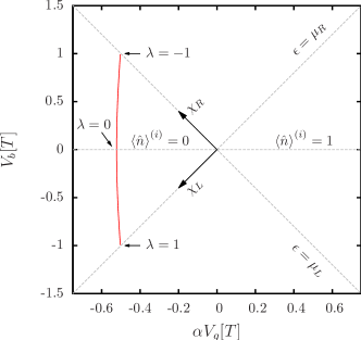
Figure 4: Position of the low-bias peak (1) of the pseudo magnetic field as function of the junction asymmetry. The curve shown here, given by Eq. (42), cannot be distinguished from the exact one.

The extension of the above analysis to peak (3) in Fig. 3 is straightforward. In this case, we set the origin of coordinates at the point $(\alpha V_{g},V_{b})=(U,0)$ and the resulting pseudo magnetic field can then be related to the one of Eq. (41) by

$$\mathcal{B}_{I_{L}}^{(U,0)}(\chi_{L},\chi_{R})=-\mathcal{B}_{I_{L}}^{(0,0)}(-\chi_{L},-\chi_{R}).$$ (45)

The negative sign in the above equation indicates that now the loading part dominates the cycle. Due to this sign, we now look at the points that minimize the field here. According to the inversion of the sign in the driving parameters, these points are the ones of Eq. (42) but with opposite sign. Therefore, since we took the origin at $(\alpha V_{g},V_{b})=(U,0)$, the peak (3) is shifted into the $N=2$ Coulomb diamond, such that for $\lambda=0$, the peak is located at $\alpha V_{g}\simeq U+0.522~{}T$ and $V_{b}=0$. Finally, when taking finite values of $\lambda$, the shift of the position of the peak (3) as a function of the bias is opposite to the one observed in the peak (1). In this sense, for $\lambda\rightarrow-1$ the peak approaches to $(\alpha V_{g},V_{b})=(U+T/2,-T)$ and when $\lambda\rightarrow 1$ it sits close to $(U+T/2,T)$.

We now calculate the maximal pumped charge as obtained from Eqs. (23)-(24) when the working point is set in the position where the peak is maximum [see Eq. (42)]. We consider a circular trajectory $\partial\Sigma$ for the driving parameters as defined in Eq. (4). The numerical evaluation of the pumped charge $Q_{I_{L}}^{(0,0)}$ related to the peak (1) is depicted in Fig. 5 as a function of the modulation amplitude $\delta\chi$, i.e. the radius of the circle over which the field is integrated. We observe that, regardless of the value of $\lambda$ or $\delta\chi$, the sign of the pumped charge is fixed only by the direction of the pumping cycle. As we will show in the next subsection, this is not the case at high-bias, where the pumped charge shows a strong dependence on $\lambda$.

For small driving amplitudes, i.e. $\delta\chi\ll 1$, the pumped charge is proportional to the area $\Sigma$ encircled by the trajectory $\partial\Sigma$ of the driving cycle, in agreement with Refs. Brouwer98, ; Aleiner98, . For an arbitrary junction asymmetry, this can be approximated by

$$Q_{I_{L}}^{(0,0)}\simeq(1-\lambda^{2})\mathcal{B}_{I_{L}}^{\mathrm{max}}\pi\delta\chi^{2},$$ (46)

where $\mathcal{B}_{I_{L}}^{\mathrm{max}}\simeq 0.0106$ is the maximum value of the peak for $\lambda=0$.

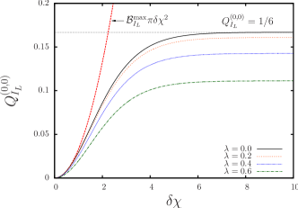
Figure 5: (Color online) Pumped charge in the low bias regime as function of the modulation amplitude $\delta\chi$ for several values of the junction asymmetry. For $\lambda=0$, the regimes of small and large driving amplitudes [see Eqs. (46) and (47)] are indicated by dashed red and gray lines respectively.

When increasing the amplitude, the driving parameters start exploring regions which are away from the crossing point of the two resonance lines and the pumped charge no longer follows the above relation. In this large amplitude (but still adiabatic) driving regime, characterized by $\delta\chi\gtrsim 1$, it is important to remark that the adiabaticity condition $\Omega\delta\chi\ll T$ is still preserved, since we can always take arbitrary small values for the modulation frequency without affecting $Q_{I_{L}}$. When evaluating the pseudo magnetic field in Eq. (39) for $\chi_{r}\gg 1$, the exponential decay implies an asymptotic value for the pumped charge, as shown in Fig. 5. In this case, the particular choice of the working point and the specific shape of the trajectory in the parameter space become irrelevant as far as the peak is fully contained in $\Sigma$. The pumped charge then saturates atnote2

$$Q_{I_{L}}^{(0,0)}\simeq\frac{3}{2}\frac{1-\lambda^{2}}{9-\lambda^{2}}.$$ (47)

It shows a quadratic dependence on $\lambda$ for $\lambda\ll 1$, in agreement with Fig. 5. The maximum value of the pumped charge, corresponding to $\lambda=0$, is

$$Q_{I_{L}}^{(0,0)}|_{\mathrm{max}}=\frac{1}{6},$$ (48)

in units of the electronic charge. To explain this particular value and to illustrate the mechanism of pumping at low bias we show, in Fig. 6, the time-resolved average charge and response coefficient during a cycle of the modulation around the working point $(\alpha\bar{V}_{g},\bar{V}_{b})=(0,0)$. We divide the cycle into four steps corresponding to the different regions of the stability diagram visited by the driving parameters. Here we consider a symmetric coupling to the leads ($\lambda=0$). The four regions are:

1. Turning point (meaning that the dot level takes its maximum or minimum value) above the chemical potentials: $\epsilon>\mu_{r}$. The $\gamma_{r}$ factors are exponentially suppressed and $\varphi_{n}^{I_{r}}=-1/2$.

2. Going down between the chemical potentials: $\mu_{L}<\epsilon<\mu_{R}$. Here $\gamma_{L}\simeq 0$ and $\gamma_{R}\simeq\Gamma/2$, such that $\varphi_{n}^{I_{L}}=-1/3$ and $\varphi_{n}^{I_{R}}=-2/3$.

3. Turning point below: $\epsilon<\mu_{r}$. Here $\gamma_{r}\simeq\Gamma/2$ and the same response coefficients are obtained. As in a), these are $-1/2$.

4. Going up through $\mu_{R}<\epsilon<\mu_{L}$, the asymmetric situation observed in b) is reversed and we obtain $\varphi_{n}^{I_{L}}=-2/3$ and $\varphi_{n}^{I_{R}}=-1/3$.

To estimate the pumped charge, we consider the time-integral of the current given in Eq. (38) noting that, in the large amplitude driving regime, the time-derivative of $\braket{\hat{n}}_{t}^{(i)}$ is only nonzero when crossing a resonance line. This last derives from the blocking of certain transitions by the Coulomb interaction. Therefore, we can approximate $d\braket{\hat{n}}_{t}^{(i)}/dt$ through the difference between the asymptotic values obtained at each side of the resonance, while for the response coefficient we take the average between its asymptotic values before and after the crossing, i.e. $Q_{I_{L}}^{(0,0)}\simeq-5/18-5/36+7/18+7/36=1/6$. This corresponds to the maximum possible value of the pumped charge when modulating the gate and bias voltage. We observe that for this particular modulation the total pumped charge is not quantized. Such quantization of $Q_{I_{L}}^{(0,0)}$ would demand the modulation of an additional parameter (e.g. the tunnel barriers)Battista11 and is not what we address here. In general, the (measurable) plateau value that is reached does, however, provide information about the tunnel coupling asymmetry. This is similar to the use of noise values in the SET regime.Thielmann03

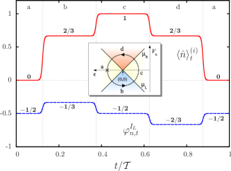
Figure 6: (Color online) Time-resolved average charge (solid red) and response coefficient (dashed blue) for $\lambda=0$ and $\delta\chi\gg 1$ during a cycle of the modulation. Inset: scheme of the explored regions of the stability diagram during the pumping cycle around the working point $(\alpha\bar{V}_{g},\bar{V}_{b})=(0,0)$.

To complete the analysis of pumping at low bias, we mention that the pumped charge $Q_{I_{L}}^{(U,0)}$ related to the peak (3) around the point $(\alpha V_{g},V_{b})=(U,0)$ reads

$$Q_{I_{L}}^{(U,0)}=-Q_{I_{L}}^{(0,0)},$$ (49)

where we used the antisymmetric shape of $\mathcal{B}_{I_{L}}$ along the particle-hole symmetry point $(\alpha V_{g},V_{b})=(U/2,0)$ [see Eq. (45) and Appendix A].

III.3.2 High-bias regime

Now we extend the above discussion to the region around a large static bias $V_{b}\sim U$, i.e. the peak (2) in Fig. 3. We evaluate the pseudo magnetic field and the resulting pumped charge when encircling the crossing point [cf. Eq. (4)] $(\alpha V_{g},V_{b})=(U/2,U)$, which is taken as the new origin of coordinates for the voltages. In this regime, the resulting pseudo magnetic field can be written in terms of the low-bias field as

$$\mathcal{B}_{I_{L}}^{(U/2,U)}(\chi_{L},\chi_{R})=\lambda\,\mathcal{B}_{I_{L}}^{(0,0)}(-\chi_{L},\chi_{R}).$$ (50)

This relation between low- and high-bias field is a central result of this paper. As a direct consequence of the $\lambda$ prefactor, we observe that since $|\lambda|<1$, the magnitude of the peak (2) is always smaller than the one of peak (1) and its sign is uniquely determined by the sign of $\lambda$. For any two modulation curves of the same shape and direction, centered around these points and symmetric with respect to the $\chi_{R}$ axis, a change of variables allows us to write

$$\iint_{\Sigma}dS\mathcal{B}_{I_{L}}^{(U/2,U)}(\boldsymbol{\chi})=\lambda\iint_{\Sigma}dS\mathcal{B}_{I_{L}}^{(0,0)}(\boldsymbol{\chi}),$$ (51)

such that we can calculate $Q_{I_{L}}^{(U/2,U)}$ in terms of the pumped charge at low bias

$$Q_{I_{L}}^{(U/2,U)}=\lambda\,Q_{I_{L}}^{(0,0)}.$$ (52)

As noted in Ref. Reckermann10, , the mere presence of a pumped charge in the high-bias regime indicates an asymmetric coupling to the leads. Since for the chosen modulation the sign of $Q_{I_{L}}^{(0,0)}$ is always positive, the sign of $Q_{I_{L}}^{(U/2,U)}$ could be used as a quick test to determine which one of the two leads is dominating the transport. For a direct quantitative estimation of $\lambda$, one simply divides the pumped charge at the different bias regimes:

$$\frac{\Gamma_{L}-\Gamma_{R}}{\Gamma_{L}+\Gamma_{R}}=\frac{Q_{I_{L}}^{(U/2,U)}}{Q_{I_{L}}^{(0,0)}}.$$ (53)

In particular, this is convenient in the regime of large driving amplitudes, where the pumped charge is not affected by the precise details of the trajectory.

As compared to the low-bias peak (1), the $\lambda$ prefactor tells us that the loading/unloading symmetry can no longer be broken for symmetric barriers, i.e. $\lambda=0$. In fact, for this particular case, although there is a change in the response coefficient along the pumping cycle, it has the same time-dependence as the average charge, i.e.

$$\varphi_{n,t}^{I_{L}}=\frac{\braket{\hat{n}}_{t}^{(i)}}{2}-1,$$ (54)

and the adiabatic charge current is a total time-derivative. Therefore, a finite pseudo magnetic field is now a cooperative effect of a change in the response coefficient and the junction asymmetry: A finite $\lambda$ is required in order to have non-parallel gradients in Eq. (39).

Eq. 50 is also useful in that it allows us to determine the maximal pumped charge working point based entirely on the low-bias feature. According to Eq. (50), the dependence on $\lambda$ of this point follows the same condition as in the low-bias regime, except for the sign inversion of $\chi_{L}$ and the shifted origin of coordinates. Therefore, starting from the position of the peak (1) in Fig. 3, we can determine the position of the peak (2) by performing first a reflection at the resonance line $\epsilon=\mu_{L}$ and then a translation by $(U/2,U)$. Although for symmetric junctions ($\lambda=0$) there is no peak, its position would be shifted in the bias voltage by $\Delta V_{b}=2\ln[(1+\sqrt{33})/4]~{}T$ with respect to the crossing of the dot-level resonance lines at $(U/2,U)$. As soon as we increase $\lambda$ from $0$, the peak emerges and moves almost horizontally (i.e. along the gate voltage axis) towards the $\epsilon=\mu_{R}$ resonance line whereas for negative values of $\lambda$ the peak moves towards the $\epsilon=\mu_{L}$ line.

Finally, the above analysis can be transferred to the peak (4) by using the bias voltage symmetry discussed in Appendix A. In this case, the pseudo magnetic field can be written in terms of the low-bias field as

$$\mathcal{B}_{I_{L}}^{(U/2,-U)}(\chi_{L},\chi_{R})=-\lambda\mathcal{B}_{I_{L}}^{(0,0)}(\chi_{L},-\chi_{R}),$$ (55)

such that the pumped charge at this working point

$$Q_{I_{L}}^{(U/2,-U)}=-\lambda Q_{I_{L}}^{(0,0)},$$ (56)

provides an additional and independent quantitative measurement of the junction asymmetry. This can be used as a cross check on experimental results.

III.4 Finite external magnetic field

We now include a finite external magnetic field $B\gg T$. note3 In this situation, in addition to the adiabatic charge current $I_{r,t}^{(a)}$, a nonzero adiabatic spin current $J_{r,t}^{(a)}$ also flows through the dot.

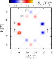
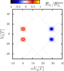
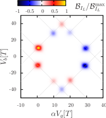
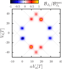
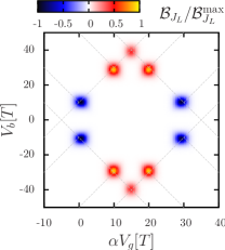
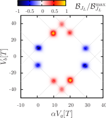
Figure 7: (Color online) Normalized pseudo magnetic fields for the pumped charge (top panels) and pumped spin (bottom panels) for junction asymmetries $\lambda=-0.25$ (left), $\lambda=0$ (center) and $\lambda=0.25$ (right). The chosen interaction energy is $U=30T$ and the external magnetic field is $B=10T$.

In Fig. 7 we show stability diagrams for the pseudo magnetic fields for the pumped charge (top panels) and the pumped spin (bottom panels) for different junction asymmetries. The external magnetic field $B=10~{}T$, where $T$ is the thermal energy, now splits the resonances of Fig. 3 into further well-separated peaks. The pseudo magnetic field is nonzero only around the meeting points of two crossing resonance lines. As in the case $B=0$, this is again because the loading/unloading symmetry is preserved when the driving is far away from any resonance line or when it only crosses a single resonance line. A simple inspection of Fig. 7 shows that, regardless of the value of $\lambda$, there is no peak in the crossing point at zero bias (black arrows in the upper left panel). In Ref. Reckermann10, , the absence of a peak was related to the lifting of the spin degeneracy in the states with single occupation. Additionally, a strong dependence on $\lambda$ in the high-bias peaks [(2) and (3) in Fig. 7] of $\mathcal{B}_{I_{L}}$ is observed.Reckermann10 In contrast, the peaks of $\mathcal{B}_{J_{L}}$ are almost unaffected by $\lambda$. The difference between charge and spin current is particularly strong for $\lambda=0$, where we find pure spin pumping in the high-bias regime: the pumped charge peaks (top center panel) vanish exactly while the ones related to the pumped spin (bottom center panel) remain finite.

To understand the above features of the pseudo magnetic fields and how they affect the pumping, we consider first the absence of a peak around $(\alpha V_{g},V_{b})=(-B/2,0)$. In this regime of the driving parameters, the charge in the quantum dot is spin polarized, such that the average charge and spin simplify to $\braket{\hat{n}}_{t}^{(i)}=p_{\uparrow,t}^{(i)}$ and $\braket{\hat{S}_{z}}_{t}^{(i)}=p_{\uparrow,t}^{(i)}/2$, respectively. Therefore, the adiabatic currents of Eqs. (25) and (29) simplify to

$$I_{L,t}^{(a)} =-\frac{\Gamma_{L}}{\Gamma}\frac{d}{dt}\braket{\hat{n}}_{t}^{(i)},$$ (57a)

$$J_{L,t}^{(a)} =\frac{1}{2}I_{L,t}^{(a)}.$$ (57b)

Since in this regime there is a single available transition, namely, $\ket{0}\leftrightarrow\ket{\uparrow}$, the relative rate at which the dot is loaded has to be the same as the one during the unloading. In the language of the vector fields, the vector potential $\mathbfcal{A}_{R}$ associated with these currents is irrotational, such that integration over the closed trajectory yields zero pumped charge. As compared to the $B=0$ result at low bias (see Sec. III.3.1), a finite pumped charge requires not only a modulation encircling the meeting point of two resonance lines but also a change in the spin degeneracy of the ground state.

We now investigate the regions in which the pseudo magnetic field is nonzero. We consider first the peak labeled by (1) in Fig. 7. Here, the two transitions $\ket{0}\leftrightarrow\ket{\uparrow}$ and $\ket{0}\leftrightarrow\ket{\downarrow}$ are enabled by the bias window $\mu_{L}-\mu_{R}$ such that the spin degeneracy in the $N=1$ charge block is effectively recovered and the loading/unloading symmetry is again broken. To calculate the pseudo magnetic fields associated with the charge ($\mathcal{B}_{I_{L}}$) and spin ($\mathcal{B}_{J_{L}}$) currents, we set the origin of coordinates at the crossing point $(\alpha V_{g},V_{b})=(0,B)$. Although the explicit expression for the fields is cumbersome, these show the simple relation

$$\mathcal{B}_{J_{L}}^{(0,B)}(\boldsymbol{\chi})=-\frac{1}{2}\mathcal{B}_{I_{L}}^{(0,B)}(\boldsymbol{\chi}),$$ (58)

for arbitrary junction asymmetries. By calculating the corresponding pumped charge and spin, and noticing that these follow the same relation as the fields, we can describe the spin resolved pumped charge through the definitions

$$Q_{I_{L}^{\uparrow}}=\frac{Q_{I_{L}}+2Q_{J_{L}}}{2},$$ (59a)

$$Q_{I_{L}^{\downarrow}}=\frac{Q_{I_{L}}-2Q_{J_{L}}}{2}.$$ (59b)

Since in this regime $Q_{J_{L}}^{(0,B)}=-Q_{I_{L}}^{(0,B)}/2$, the pumped charge is purely given by spin $\downarrow$ carriers. To estimate the dependence on $\lambda$, we calculate $Q_{I_{L}}^{(0,B)}$ for a large driving amplitude and obtain

$$Q_{I_{L}}^{(0,B)}=\frac{1+\lambda}{3+\lambda}.$$ (60)

Notice that, for the chosen modulation, the sign of the pumped charge is always positive, regardless of the particular value of $\lambda$. Since no charge is accumulated after one period of the modulation, i.e. $Q_{I_{L}}^{(0,B)}+Q_{I_{R}}^{(0,B)}=0$, the charge is pumped from the right lead to the left lead. In this case, the breaking of the loading/unloading symmetry in both the charge and spin in the dot is mainly due to the change in the number of available transitions. This affects the value of the response coefficients in such a way that the total amount of charge leaving the left lead during the loading part of the cycle is smaller than the one entering the same lead during the unloading. This is illustrated in Fig. 8, for the case $\lambda=0$ and $\delta\chi\gg 1$, where we show the average charge and spin in the dot together with the corresponding response coefficients. According to Eq. (60), the pumped charge for $\lambda=0$ corresponds to $1/3$ of the electronic charge. This limit can be understood from the asymptotic values shown in Fig. 8, in a similar way as we did in the previous section for $Q_{I_{L}}^{(0,0)}$. The difference now is that the pumped charge is not only subjected to a change in the average charge of the dot, but also to the variation of the average spin. In particular, the loading (unloading) of the spin does not necessarily correlate with the loading (unloading) of the charge. Therefore we must distinguish the two contributions. The estimation of the time-derivatives of the average charge and spin, together with the average value of the response coefficients each time the driving parameters cross a resonance line (gray dashed lines in Fig. 8) yields

$$Q_{I_{L}}^{(0,B)}=1/48+15/48=1/3,$$ (61)

with the first term related to the variation of the average charge and the second to the average spin.

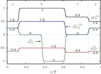
Figure 8: (Color online) Time-resolved average charge (solid black) and spin (solid blue) together with the charge current response coefficients $\varphi_{n,t}^{I_{L}}$ (dashed red) and $\varphi_{s,t}^{I_{L}}$ (dashed green) for $\lambda=0$ and $\delta\chi\gg 1$ during a cycle of the modulation around the working point $(0,B)$.

The above discussed value $1/3$ for the maximal pumped charge can be increased or decreased depending on the sign of the junction asymmetry [see Eq. (60)]. For positive $\lambda$, the maximal pumped charge increases from $1/3$ to $1/2$. However, in the extreme case $\lambda\simeq 1$ the (negative) peak (2) approaches the region of integration and its contribution can no longer be disregarded.

We now consider the pumped charge and spin in the high-bias limit, characterized by the peaks (2) and (3) in Fig. 7. To keep the notation simple, we now use the index (2) to indicate that the origin of coordinates is set at the point $(\alpha V_{g},V_{b})=((U-B)/2,U)$. In the regime of large driving amplitude we obtain

$$Q_{J_{L}}^{(2)} =\frac{1}{2}\frac{(1+\lambda)^{2}(3-\lambda)}{(3+\lambda)(3+\lambda^{2})},$$ (62a)

$$Q_{I_{L}}^{(2)} =-2\lambda Q_{J_{L}}^{(2)}.$$ (62b)

Therefore, since the pumped spin is always positive, the resulting pumped charge changes its sign in the symmetry point $\lambda=0$. Notice that the regime of validity of the above limit includes $|\lambda|<1$. For $\lambda\simeq 1$ we should consider the contribution from the peak (1), such that both the pumped charge and spin go to zero. By using Eq. (59), the spin resolved current shows to be decomposed into contributions from spin $\uparrow$ carriers flowing from the right lead to the left lead and spin $\downarrow$ carriers flowing in the opposite direction. The ratio between these two contributions depends on $\lambda$ via

$$\left|\frac{Q_{I_{L}^{\uparrow}}^{(2)}}{Q_{I_{L}^{\downarrow}}^{(2)}}\right|=\frac{1-\lambda}{1+\lambda},$$ (63)

such that for $\lambda<0$ ($>0$) the transport is dominated by spin $\uparrow$ ($\downarrow$) carriers. Remarkably, for a symmetrically coupled dot we obtain pure spin pumping, since the two contributions are exactly opposite and therefore the pumped charge is zero. In this case, the limit $\delta\chi\gg 1$ yields

$$Q_{J_{L}}^{(2)}=\frac{1}{6},$$ (64)

which can again be understood in terms of the asymptotic values of the response coefficients and the instantaneous average charge and spin as we previously demonstrated for $Q_{I_{L}}^{(0,B)}$ [see Eq. (61)].

Finally, we analyze pumping for large driving amplitudes around the peak (3), given by the crossing of the resonance lines at $(\alpha V_{g},V_{b})=(U/2,U+B)$. Now the relation between the pumped charge and spin is non-trivial:

$$Q_{I_{L}}^{(3)} =\lambda\frac{1-\lambda^{2}}{3+\lambda^{2}},$$ (65a)

$$Q_{J_{L}}^{(3)} =\frac{1}{4}(1-\lambda^{2})\frac{3+4\lambda^{2}+\lambda^{4}}{(3+\lambda^{2})^{2}}.$$ (65b)

It implies a positive sign for the pumped spin while the pumped charge again changes its sign with the sign of $\lambda$. Despite this, the spin resolved pumped charge, calculated by Eq. (59), obeys $Q_{I_{L}^{\downarrow}}^{(3)}(\lambda)=-Q_{I_{L}^{\uparrow}}^{(3)}(-\lambda)$. As in the previously studied regime around the peak (2), symmetric coupling to the leads yields a pure pumped spin, which in this case is

$$Q_{J_{L}}^{(3)}=\frac{1}{12}.$$ (66)

The difference with the situation around the peak (2) is that now, for $\lambda<0$ ($>0$), the transport is dominated by $\downarrow$ ($\uparrow$) carriers.

Finally, we note that the above discussion of peaks (1)-(3) can be extended to all remaining peaks in Fig. 7 by using general gate- and bias-voltage symmetries of the problem in an external magnetic field which are presented in Appendix A.

IV Conclusions

We investigated adiabatic charge and spin pumping through an interacting quantum dot driven out of equilibrium by a non-linear bias voltage and time-dependent parameter modulations. We showed that, regardless of the specific modulation, the time-resolved adiabatic charge and spin currents can be interpreted as the response to a perturbation in the instantaneous average charge and spin due to the variation of the driving parameters. This allowed us to identify the charge and spin emissivities to the leads in the context of interacting systems in the non-linear transport regime.

For the specific case of a modulation of the gate and bias voltage, we discussed the conditions for interaction-induced pumping in terms of the properties of vector fields associated to the adiabatic charge and spin currents. We observed that the Coulomb interaction is crucial since it gives the rotational contribution to the pseudo vector potential that cannot be gauged away: It generates a nonzero pseudo magnetic field and in consequence a finite pumped charge. For a single-level quantum dot, we explored the stability diagram associated to this vector field for arbitrary bias and junction asymmetry. The shape of the pseudo magnetic field reflects the two-parameter condition required for adiabatic pumping, such that it shows a maximum whenever two lines of the usual $dI/dV$ stability diagram meet. The analytic expressions for the pseudo magnetic field and the pumped charge enable detailed fitting of experimental results. For low bias voltages, the pumping mechanism is dominated by the change in the response coefficient when exploring different regions of the pumping cycle. In constrast, in the high-bias regime, the finite pumped charge is generated by the cooperative effect of the above mechanism and the junction asymmetry. This allows for a direct quantitative determination of the junction asymmetry by two measurements of the pumped charge.

The role of the external magnetic field was found to be twofold: First, it restores at low bias the loading/unloading symmetry previously broken by the local interaction in combination with the spin-degeneracy. This is evidenced by a suppression of the pumped charge at zero bias. Second, in addition to the pumped charge, a pumped spin arises once the spin degeneracy is effectively recovered through an applied bias. In particular, the weak dependence of the pumped spin on the junction asymmetry allows for pure spin pumping in the high-bias regime.

Appendix A Applied voltage symmetries

In order to completely characterize the adiabatic transport of charge and spin along the full stability diagram, we derive the reflection symmetries of the pseudo magnetic fields $\mathcal{B}_{I_{L}}$ and $\mathcal{B}_{J_{L}}$. Specifically, we study the behavior of $\mathcal{B}_{R}$ with respect to: (i) the reversal of the bias voltage $V_{b}\rightarrow-V_{b}$ and, (ii) the reversal of the gate voltage $\alpha V_{g}\rightarrow U/2-\alpha V_{g}$. To simplify the notation, we use $v=V_{b}/2$. These symmetries derive from the interchange of the two electrodes and the particle-hole symmetry of a single interacting level. Although not exact anymore for multi-level quantum-dots, we expect similar qualitative correspondences to hold in general.

A.1 Bias voltage reversal

We write the coupling strength in terms of the junction asymmetry by $\Gamma_{r}(\lambda)=\Gamma(1+\alpha_{r}\lambda)/2$, with $\alpha_{r}=\pm$ for $r=L,R$ respectively. The factors in Eq. (27) then obey the following relations

$$\gamma_{r}(\epsilon,-v,\lambda) =\gamma_{\bar{r}}(\epsilon,v,-\lambda),$$ (67a)

$$\beta_{r}(\epsilon,-v,\lambda) =\beta_{\bar{r}}(\epsilon,v,-\lambda),$$ (67b)

where $\bar{r}=R(L)$ for $r=L(R)$ and $\epsilon=-\alpha V_{g}$. By plugging these into the definitions of the charge current response coefficients [see Eq. (26)] we obtain

$$\varphi_{n}^{I_{L}}(\epsilon,-v,\lambda) =-1-\varphi_{n}^{I_{L}}(\epsilon,v,-\lambda),$$ (68a)

$$\varphi_{S_{z}}^{I_{L}}(\epsilon,-v,\lambda) =-\varphi_{S_{z}}^{I_{L}}(\epsilon,v,-\lambda),$$ (68b)

and for the spin current response coefficients of Eq. (30) we have

$$\varphi_{n}^{J_{L}}(\epsilon,-v,\lambda) =-\varphi_{n}^{J_{L}}(\epsilon,v,-\lambda),$$ (69a)

$$\varphi_{S_{z}}^{J_{L}}(\epsilon,-v,\lambda) =-1-\varphi_{S_{z}}^{J_{L}}(\epsilon,v,-\lambda).$$ (69b)

Now we repeat this analysis for the average charge and spin. The explicit expressions of these two quantities for arbitrary $U$ and $B$ can be calculated from the instantaneous occupation probabilities $\mathbf{p}_{t}^{(i)}$ obtained as the solution to Eq. (9). These write as follows

$$\braket{\hat{n}}^{(i)} =\frac{\sum_{r\sigma}\Gamma_{r}f(\epsilon_{r\bar{\sigma}})(\Gamma-2\gamma_{\sigma})}{\Gamma^{2}-\gamma^{2}+\beta^{2}},$$ (70a)

$$\braket{\hat{S}_{z}}^{(i)} =\frac{1}{2}\frac{\sum_{rr^{\prime}\sigma}\Gamma_{r}\Gamma_{r^{\prime}}f(\epsilon_{r\sigma})f^{-}(\epsilon_{r\bar{\sigma}}+U)}{\Gamma^{2}-\gamma^{2}+\beta^{2}},$$ (70b)

where $\bar{\sigma}=-\sigma$, $f^{-}(\omega)=f(-\omega)$, with $f(\omega)=[1+\exp(\omega/T)]^{-1}$ and $\gamma_{\sigma}=\sum_{r}\Gamma_{r}/2[f(\epsilon_{r\sigma})-f(\epsilon_{r\sigma}+U)]$. For these averages, a change in the sign of the bias voltage is equivalent to an inversion of the tunnel barriers, i.e.

$$\braket{\hat{n}}^{(i)}(\epsilon,-v,\lambda) =\braket{\hat{n}}^{(i)}(\epsilon,v,-\lambda)$$ (71a)

$$\braket{\hat{S}_{z}}^{(i)}(\epsilon,-v,\lambda) =\braket{\hat{S}_{z}}^{(i)}(\epsilon,v,-\lambda).$$ (71b)

In the calculation of the gradients of such quantities, we notice that

$$\left(\partial_{\epsilon}\varphi\right)(\epsilon,-v,\lambda) =-\left(\partial_{\epsilon}\varphi\right)(\epsilon,v,-\lambda),$$ (72a)

$$\left(\partial_{v}\varphi\right)(\epsilon,-v,\lambda) =\left(\partial_{v}\varphi\right)(\epsilon,v,-\lambda),$$ (72b)

for the response coefficients and

$$\left(\partial_{\epsilon}\braket{\hat{R}}^{(i)}\right)(\epsilon,-v,\lambda) =\left(\partial_{\epsilon}\braket{\hat{R}}^{(i)}\right)(\epsilon,v,-\lambda),$$ (73a)

$$\left(\partial_{v}\braket{\hat{R}}^{(i)}\right)(\epsilon,-v,\lambda) =-\left(\partial_{v}\braket{\hat{R}}^{(i)}\right)(\epsilon,v,-\lambda),$$ (73b)

for the average charge and spin. The pseudo magnetic fields then write as follows

$$\mathcal{B}_{I_{L}}(\epsilon,-v,\lambda) =\mathcal{B}_{I_{L}}(\epsilon,v,-\lambda),$$ (74a)

$$\mathcal{B}_{J_{L}}(\epsilon,-v,\lambda) =\mathcal{B}_{J_{L}}(\epsilon,v,-\lambda).$$ (74b)

These two relations can be directly checked by comparing the left and right panels of Fig. 7. For $\lambda=0$ (see central panels) the above equations imply a symmetric shape of the pseudo magnetic fields around the zero-bias axis.

A.2 Gate voltage reversal

We calculate now the pseudo magnetic fields for an inversion of the gate voltage around $V_{g}=U/2$. In this case, we take as the new origin of coordinates the point $(\alpha V_{g},V_{b})=(U/2,0)$ such that the factors in Eq. (27) write

$$\gamma_{r}(\epsilon,v,\lambda) =\sum_{\sigma}\tfrac{\Gamma_{r}(\lambda)}{2}\left[f(\epsilon_{r\sigma}-\tfrac{U}{2})-f(\epsilon_{r\sigma}+\tfrac{U}{2})\right],$$ (75a)

$$\beta_{r}(\epsilon,v,\lambda) =\sum_{\sigma}\sigma\tfrac{\Gamma_{r}(\lambda)}{2}\left[f(\epsilon_{r\sigma}-\tfrac{U}{2})-f(\epsilon_{r\sigma}+\tfrac{U}{2})\right],$$ (75b)

where $\epsilon_{r\sigma}=\epsilon-\alpha_{r}v-\sigma B/2$. For these new coordinates, the inversion of the gate voltage is then given by $\epsilon\rightarrow-\epsilon$, and the above factors are transformed according to

$$\gamma_{r}(-\epsilon,v,\lambda) =\gamma_{\bar{r}}(\epsilon,v,-\lambda),$$ (76a)

$$\beta_{r}(-\epsilon,v,\lambda) =-\beta_{\bar{r}}(\epsilon,v,-\lambda).$$ (76b)

In consequence, the response coefficients obey the following relations

$$\varphi_{n}^{I_{L}}(-\epsilon,v,\lambda) =-1-\varphi_{n}^{I_{L}}(\epsilon,v,-\lambda),$$ (77a)

$$\varphi_{S_{z}}^{I_{L}}(-\epsilon,v,\lambda) =\varphi_{S_{z}}^{I_{L}}(\epsilon,v,-\lambda),$$ (77b)

$$\varphi_{n}^{J_{L}}(-\epsilon,v,\lambda) =\varphi_{n}^{J_{L}}(\epsilon,v,-\lambda),$$ (77c)

$$\varphi_{S_{z}}^{J_{L}}(-\epsilon,v,\lambda) =-1-\varphi_{S_{z}}^{J_{L}}(\epsilon,v,-\lambda).$$ (77d)

For the average charge and spin we obtain

$$\braket{\hat{n}}^{(i)}(-\epsilon,v,\lambda) =2-\braket{\hat{n}}^{(i)}(\epsilon,v,-\lambda),$$ (78a)

$$\braket{\hat{S}_{z}}^{(i)}(-\epsilon,v,\lambda) =\braket{\hat{S}_{z}}^{(i)}(\epsilon,v,-\lambda),$$ (78b)

such that the pseudo magnetic fields present different symmetries with respect to a change in the gate voltage, i.e.

$$\mathcal{B}_{I_{L}}(-\epsilon,v,\lambda) =-\mathcal{B}_{I_{L}}(\epsilon,v,-\lambda),$$ (79a)

$$\mathcal{B}_{J_{L}}(-\epsilon,v,\lambda) =\mathcal{B}_{J_{L}}(\epsilon,v,-\lambda).$$ (79b)

Appendix B Maximum values of $\mathcal{B}_{I_{L}}$

In this section we calculate the point in which the pseudo magnetic field is maximum, i.e. the position of the peak (1) in Fig. 3. Our starting point is the explicit form of the pseudo magnetic field at low bias. According to Eq. (41), the condition for an extremum point $(\chi_{L},\chi_{R})$ of the pseudo magnetic field is the following:

$$\tanh\left(\frac{\chi_{L}}{2}\right) =\frac{-3(1+\lambda)\partial_{\chi_{L}}f_{L}}{2+(1+\lambda)f_{L}+(1-\lambda)f_{R}},$$ (80a)

$$\tanh\left(\frac{\chi_{R}}{2}\right) =\frac{-3(1-\lambda)\partial_{\chi_{R}}f_{R}}{2+(1+\lambda)f_{L}+(1-\lambda)f_{L}},$$ (80b)

where $f_{r}=f(\chi_{r})$, $r=L,R$. Now we take the replacements $x=1+e^{\chi_{L}}$ and $y=1+e^{\chi_{R}}$, such that $x,y>1$ and the above equations read

$$3(1+\lambda)y =\frac{x-2}{x-1}(2xy+x+y+\lambda(y-x)),$$ (81a)

$$3(1-\lambda)x =\frac{y-2}{y-1}(2xy+x+y+\lambda(y-x)).$$ (81b)

By solving the first equation, we obtain

$$y=-\frac{(1-\lambda)x(x-2)}{2x^{2}-2(3+\lambda)x+1+\lambda},$$ (82)

and plugging this into the second equation we obtain the following quartic equation for $x$:

$$ax^{4}+bx^{3}+cx^{2}+dx+e=0,$$ (83)

with

$$a =2\lambda-6, b =-\lambda^{2}-4\lambda+29,$$ (84a)

$$c =2\lambda^{2}-34, d =-2(\lambda+1)^{2},$$ (84b)

$$e =(\lambda+1)^{2}.$$ (84c)

For the particular case of symmetric junctions, the solutions compatible to the condition $x>1$ are $x=(5+\sqrt{33})/4$ and $x=(7+\sqrt{37})/6$ respectively. Now if we use these values in Eq. (82), the only solution that fulfills the condition $y>1$ is $y=x=(5+\sqrt{33})/4$. Therefore, for symmetric junctions, the maximum of the pseudo magnetic field is located at the point $\chi_{L}=\chi_{R}=\ln[(1+\sqrt{33})/4]$.

References

- (1) D. J. Thouless, Phys. Rev. B 27, 6083 (1983).
- (2) B. L. Altshuler and L. I. Glazman, Science 283, 1864 (1999)
- (3) J. E. Avron, A. Elgart, G. M. Graf, and L. Sadun, Phys. Rev. B 62, 10618(R) (2000).
- (4) Y. Makhlin and A. D. Mirlin, Phys. Rev. Lett. 87, 276803 (2001).
- (5) H.-Q. Zhou, S. Y. Cho, and R. H. McKenzie, Phys. Rev. Lett. 91, 186803 (2003).
- (6) Q. Niu and D. J. Thouless J. Phys. A 17, 2453 (1984).
- (7) J. E. Avron, A. Elgart, G. M. Graf, and L. Sadun, Phys. Rev. Lett. 87, 236601 (2001).
- (8) L. P. Kouwenhoven, A. T. Johnson, N. C. van der Vaart, C. J. P. M. Harmans, and C. T. Foxon, Phys. Rev. Lett. 67, 1626 (1991).
- (9) H. Pothier, P. Lafarge, C. Urbina, D. Esteve, and M. H. Devoret, Europhys. Lett. 17, 249 (1992).
- (10) S. J. Chorley, J. Frake, C. G. Smith, G. A. C. Jones, and M. R. Buitelaar, Appl. Phys. Lett. 100, 143104 (2012).
- (11) M. W. Keller, J. M. Martinis, R. L. Kautz, Phys. Rev. Lett. 80, 4530 (1998); S. P. Giblin, M. Kataoka, J. D. Fletcher, P. See, T. J. B. M. Janssen, J. P. Griffiths, G. A. C. Jones, I. Farrer, and D. A. Ritchie, Nat. Comm. 3, 930 (2012).
- (12) G. Fève, A. Mahé, J.-M. Berroir, T. T. Kontos, B. Plaçais, D. C. Glattli, A. Cavanna, B. Etienne, and Y. Jin, Science 316, 1169 (2007).
- (13) C. W. J. Beenakker, M. Titov, and B. Trauzettel, Phys. Rev. Lett. 94, 186804 (2005).
- (14) P. Samuelsson and M. Büttiker, Phys. Rev. B 71, 245317 (2005).
- (15) J. Splettstoesser, M. Moskalets, and M. Büttiker, Phys. Rev. Lett. 103, 076804 (2009).
- (16) Y. Sherkunov, N. d’Ambrumenil, P. Samuelsson, and M. Büttiker, Phys. Rev. B 85, R081108 (2012).
- (17) F. Zhou, B. Spivak, and B. Altshuler, Phys. Rev. Lett. 82, 608 (1999).
- (18) M. Switkes, C. M. Marcus, K. Campman, and A.C. Gossard, Science 283, 1905 (1999).
- (19) S. K. Watson, R. M. Potok, C. M. Marcus, and V. Umansky, Phys. Rev. Lett. 91, 258301 (2003).
- (20) N. E. Fletcher, J. Ebbecke, T. J. B. M. Janssen, F. J. Ahlers, M. Pepper, H. E. Beere, and D. A. Ritchie, Phys. Rev. B 68, 245310 (2003); A. M. Robinson, V. I. Talyanskii, M. Pepper, J. E. Cunningham, E. H. Linfield, and D. A. Ritchie Phys. Rev. B 65, 045313 (2002).
- (21) P. W. Brouwer, Phys. Rev. B 58, 10135(R) (1998).
- (22) M. Büttiker, H. Thomas, and A. Pêtre, Z. Phys. B 94, 133 (1994).
- (23) See, for example, M. Büttiker, J. Phys.: Condens. Matter 5, 9361 (1993).
- (24) M. Moskalets and M. Büttiker, Phys. Rev. B 66, 035306 (2002).
- (25) E. R. Mucciolo, C. Chamon, and C. M. Marcus, Phys. Rev. Lett. 89, 146802 (2002); M. Governale, F. Taddei, and R. Fazio, Phys. Rev. B 68, 155324 (2003).
- (26) J. Wang, Y. Wei, B. Wang, and H. Guo, Appl. Phys. Lett. 79, 3977 (2001); M. Blaauboer, Phys. Rev. B 65, 235318 (2002); F. Taddei, M. Governale, and R. Fazio, ibid. 70, 052510 (2004).
- (27) Y. Levinson, O. Entin-Wohlman, and P. Wölfle, Phys. Rev. Lett. 85, 634 (2000); O. Entin-Wohlman, Y. Levinson, and P. Wölfle, Phys. Rev. B 64, 195308 (2001).
- (28) E. Prada, P. San-Jose, and H. Schomerus, Phys. Rev. B 80, 245414 (2009); R. Zhu and H. Chen, Appl. Phys. Lett. 95, 122111 (2009); R. P. Tiwari and M. Blaauboer, ibid. 97, 243112 (2010); E. S. Grichuk and E. A. Manykin, JETP Letters 93, 372 (2011); J.-F. Liu and K. S. Chan, Nanotechnology 22, 395201 (2011).
- (29) R. Citro, N. Andrei, and Q. Niu, Phys. Rev. B 68, 165312 (2003); S. Das and S. Rao, ibid. 71, 165333(2005).
- (30) T. Aono, Phys. Rev. Lett. 93, 116601 (2004).
- (31) A. Schiller and A. Silva, Phys. Rev. B 77, 045330 (2008).
- (32) L. Arrachea, A. Levy Yeyati, and A. Martin-Rodero, Phys. Rev. B 77, 165326 (2008).
- (33) I. L. Aleiner and A. V. Andreev, Phys. Rev. Lett. 81, 1286 (1998);
- (34) P. W. Brouwer, A. Lamacraft, and K. Flensberg, Phys. Rev. B 72, 075316 (2005).
- (35) E. Cota, R. Aguado, and G. Platero, Phys. Rev. Lett. 94, 107202 (2005); 94, 229901(E) (2005).
- (36) J. Splettstoesser, M. Governale, J. König, and R. Fazio, Phys. Rev. Lett. 95, 246803 (2005); D. Fioretto and A. Silva, ibid. 100, 236803 (2008); A. R. Hernández , F. A. Pinheiro, C. H. Lewenkopf, and E. R. Mucciolo, Phys. Rev. B 80, 115311 (2009).
- (37) E. Sela and Y. Oreg, Phys. Rev. Lett. 96, 166802 (2006).
- (38) J. Splettstoesser, M. Governale, J. König, and R. Fazio, Phys. Rev. B 74, 085305 (2006).
- (39) J. Splettstoesser, M. Governale, and J. König, Phys. Rev. B 77, 195320 (2008).
- (40) F. Cavaliere, M. Governale, and J. König, Phys. Rev. Lett. 103, 136801 (2009).
- (41) N. Winkler, M. Governale, and J. König, Phys. Rev. B 79, 235309 (2009).
- (42) R.-P. Riwar and J. Splettstoesser, Phys. Rev. B 82, 205308 (2010).
- (43) F. Reckermann, J. Splettstoesser, and M. R. Wegewijs, Phys. Rev. Lett. 104, 226803 (2010).
- (44) R.-P. Riwar, J. Splettstoesser, and J. König, (unpublished).
- (45) F. Reckermann, M. R. Wegewijs, R. Saptsov, and J. Splettstoesser, (unpublished).
- (46) O. Kashuba, H. Schoeller, and J. Splettstoesser, EPL 98, 57003 (2012).
- (47) M. Moskalets and M. Büttiker, Phys. Rev. B 69, 205316 (2004).
- (48) O. Entin-Wohlman, A. Aharony, and Y. Levinson, Phys. Rev. B 65, 195411 (2002).
- (49) T. Yuge, T. Sagawa, A. Sugita, and H. Hayakawa, arXiv:1208.3926v1 (unpublished).
- (50) A-P. Jauho, N. S. Wingreen, and Y. Meir, Phys. Rev. B 50, 5528 (1994).
- (51) J. König, H. Schoeller, and G. Schön, Phys. Rev. Lett. 76, 1715 (1996); J. König, J. Schmid, H. Schoeller, and G. Schön, Phys. Rev. B 54, 16820 (1996).
- (52) The instantaneous component simply consists of the time-averaged stationary flow and is not discussed here.
- (53) A. Brataas, Y. Tserkovnyak, G. E. W. Bauer, and P. J. Kelly, in Spin Current, edited by S. Maekawa, S. O. Valenzuela, E. Saitoh, and T. Kimura (Oxford University Press, in press).
- (54) D. Cohen, Phys. Rev. B 68, 201303(R) (2003).
- (55) D. V. Averin and K. K. Likharev, in Mesoscopic Phenomena in Solids, edited by B. Altshuler, P. A. Lee, and R. A. Webb (North-Holland, Amsterdam, 1991).
- (56) C. Bruder and H. Schoeller, Phys. Rev. Lett. 72, 1076 (1994).
- (57) S. Kohler, J. Lehmann, and P. Hänggi, Phys. Rep. 406, 379 (2005); L. E. F. Foa Torres, Phys. Rev. B 72, 245339 (2005).
- (58) E. Bonet, M. M. Deshmukh, and D. C. Ralph, Phys. Rev. B 65, 045317 (2002); M. M. Deshmukh, E. Bonet, A. N. Pasupathy, and D. C. Ralph, ibid. 65, 073301 (2002).
- (59) Since the surface integral would demand a precise knowledge of the pseudo magnetic field over the whole enclosed area, we calculate the asymptotic pumped charge as the contour integral of the vector potential introduced in Eq. (22). This has the advantage that we can first take the limit (while keeping ) in the definition of the vector potential and then calculate the pumped charge.
- (60) F. Battista and P. Samuelsson, Phys. Rev. B 83, 125324 (2011).
- (61) A. Thielmann, M. H. Hettler, J. König, and G. Schön, Phys. Rev. B 68, 115105 (2003).
- (62) The external magnetic field is indicated by the regular font and should not be confused with the pseudo magnetic field .