Squeezing and robustness of frictionless cooling strategies

Abstract

Quantum control strategies that provide shortcuts to adiabaticity are increasingly considered in various contexts including atomic cooling. Recent studies have emphasized practical issues in order to reduce the gap between the idealized models and actual ongoing implementations. We rephrase here the cooling features in terms of a peculiar squeezing effect, and use it to parametrize the robustness of frictionless cooling techniques with respect to noise-induced deviations from the ideal time-dependent trajectory for the trapping frequency. We finally discuss qualitative issues for the experimental implementation of this scheme using bichromatic optical traps and lattices, which seem especially suitable for cooling Fermi-Bose mixtures and for investigating equilibration of negative temperature states, respectively.

I Introduction

Quantum control techniques that provide shortcuts to adiabaticity, recently proposed in the atomic physics framework Chen , are experiencing rapid growth due to the necessity, in various contexts, to reduce the undesired effects of a prolonged exposure to the external environment. Such technique produces the same net result as if a full adiabatic following has been implemented, but on a much shorter timescale. More specifically, in a shortcut to adiabaticity technique the composition of eigenstates one started with is preserved at the end of the process, but not during the process, unlike full adiabatic following. The first experimental implementations have demonstrated efficient fast decompression of ⁸⁷Rb atoms in normal Schaff0 and Bose-condensed Schaff states, as well as fast atomic transport Torrontegui . Consequently, a number of contributions have focused attention on possible deviations from ideal realizations which could constitute bottlenecks to further implementations of these techniques. In one study, it was found that the transient energy excitation limits the maximum attainable speed Chen1 . In another, deviations from harmonicity in the trapping potential, with specific attention to the crosstalk between the dynamics in different trapping directions, have recently been discussed Torrontegui1 .

Our previous work Choi showed that frictionless cooling (also known as “fast adiabatic” cooling), an example of shortcut to adiabaticity technique, may be optimal in controlling the temperature of a buffer gas in the sympathetic cooling of another species, such as a Fermi gas. This is because this cooling method allows for retaining the maximum value of the gas heat capacity, both as the gas does not enter the degenerate regime, and as it avoids the intentional loss of atoms required in evaporative cooling. Even in this case, we found that practical issues may limit the successful application of this technique. Specifically, it was shown that, for short cooling times, atoms temporarily attain temperatures higher than the initial temperature before settling down to the final temperature. This can potentially result in atom losses in any realistic potential with a finite trapping depth. Also, very small final temperatures may result in a large spatial mismatch between the sizes of the two clouds making sympathetic cooling less effective. These considerations put practical restrictions on this method.

Here, we extend our analysis by studying the robustness of the frictionless cooling method with respect to the likely presence of noise in a potential experiment. This is in light of the fact that, experimentally, there may be systematic sources of error which are of a truly nonlinear nature, such as noise in the trapping frequency or anharmonicities in the trapping potential. To model the noise, we assume that an experimentalist has a well-defined protocol for implementing frictionless cooling and that the effect of various noise sources present in the apparatus (such as current noise in the coils for magnetic trapping, or laser power fluctuations in an optical dipole trap) add up to deviations from the ideal (Ermakov) trajectory.

In order to parametrize the robustness, one needs to estimate how much the eigenstate composition of the final state deviates from that of the initial state. However, usual measures such as the fidelity of the wave function ${\cal F}=|\langle\psi(t_{\mathrm{f}})|\psi(0)\rangle|$ are unsuitable in this scheme since, due to the trap relaxation, the final wave function spreads out in space significantly. To circumvent this constraint, we note that our particular frictionless cooling methodChoi can be formally linked to squeezing, and this allows us to use the amount of squeezing produced as a measure of robustness. In particular, starting from a minimum uncertainty state, frictionless cooling should result in a minimum uncertainty state at the end of the run. Any deviation may be considered an indicator of less than perfect recovery of the desired final state, i.e. a sign of an imperfect “adiabatic following.” It should be noted that there are limitations in using squeezing as a general measure of robustness in situations other than the specific cooling scheme under consideration. Specifically, one cannot easily generalize this measure to more sophisticated states, such as mixed states or non-minimal uncertainty states. As a supplementary figure of merit of robustness, we have also chosen a modified fidelity measure ${\cal F^{\prime}}=|\langle\psi(t_{f})|\psi_{target}\rangle|$ where $\psi(t_{f})$ and $\psi_{target}$ are the final states attained in the presence and in the absence of noise, respectively, and present results using this measure along with the squeezing parameter.

The paper is organized as follows: In Section II we discuss the connection of frictionless cooling to squeezing which we use as a useful indicator of the fidelity in reaching a targeted final temperature. In Section III we apply these considerations to discuss the robustness of the ideal shortcut to adiabaticity trajectories to noise fluctuations in the trapping parameters. The possible noise sources are characterized as broadband and monochromatic, and we discuss the interplay between their spectra in relation to the intrinsic spectral content of the frictionless cooling protocol. We finally provide various connections to recent developments in the control of ultracold atoms, including a qualitative discussion of the realization of frictionless cooling in a bichromatic optical trap, a promising candidate for implementing the antitrapping stage required for very fast cooling, provided that noise fluctuations in the trap are kept under control.

II Squeezing in frictionless cooling

As discussed in Ref. Chen , frictionless cooling relies on specific dynamics of the harmonic trapping frequency to transfer a quantum state such as an equilibrium thermal state in a trap of initial trapping angular frequency $\omega_{0}$ to that of final angular frequency $\omega_{\mathrm{f}}\ll\omega_{0}$. This ensures that the energy level spacings in the final trap are much smaller than those of the initial trap, hence lowering the overall temperature. As we have discussed in detail in our previous work Choi , we have additionally used the momentum variance as an indicator of temperature and have shown that the final wave function has its momentum variance reduced by a factor of $\omega_{0}/\omega_{\mathrm{f}}$ compared to that of the initial wave function. The use of the momentum variance as an indicator of the temperature in an ultracold atomic cloud has been recently validated in dedicated experiments Davis .

The shortcut to adiabaticity is accomplished using a method originally studied by Lewis and Riesenfeld Lewis0 ; Lewis , who introduced the invariant operator related to the harmonic oscillator with an arbitrary time-dependent harmonic potential, $\hat{I}(t)=(b\hat{p}-m\dot{b}\hat{q})^{2}/2m+m\omega_{0}^{2}\hat{q}^{2}/(2b^{2})$. A key feature is that the eigenstates of $\hat{I}(t)$ can be made to coincide with the eigenstates of the harmonic oscillator Hamiltonian, particularly at the beginning and at the end of the cooling process. Here $b(t)$ is a time-dependent frequency scaling factor which satisfies the Ermakov equation $\ddot{b}(t)+\omega(t)^{2}b=\omega_{0}^{2}/b^{3}$. This can be solved by imposing boundary conditions on $b(t)$ and its first and second time derivatives, while assuming both a targeted final trapping frequency $\omega_{\mathrm{f}}$, and a total time duration for the protocol, $t_{\mathrm{f}}$ Chen . This results in a well-defined Ermakov trajectory for the trap frequency $\omega(t)$. By constructing a harmonic oscillator with the Ermakov trajectory for its time-dependent trapping frequency, a ground state experiences dynamic changes in the trapping frequency that eventually results in its cooling within the specified time $t_{\mathrm{f}}$. In this paper, we shall denote the Ermakov trajectory as $\omega_{E}(t)$ in order to distinguish it from a general time-dependent trap frequency.

Formally, the above method may be understood as a transformation of a harmonic oscillator Hamiltonian to the space of the invariant operator $\hat{I}(t)$. In particular, the net effect can be considered as an added nonlinearity to the Hamiltonian that produces squeezing of atomic states. A first step in this direction has been reported in Sokolovski where number (Fock) states during sudden and adiabatic expansions of the trap have been discussed. One can show how squeezing is a natural byproduct of the Ermakov dynamics by noting the relationship between the raising and lowering operators of the harmonic oscillator Hamiltonian $a^{\dagger}(t)$ and $a(t)$, and the Dirac raising and lowering operators for the Lewis and Riesenfeld invariant operator $\hat{I}(t)$ $\alpha^{\dagger}(t)$ and $\alpha(t)$Lewis :

$$\alpha(t) = \eta(t)a(t)+\zeta(t)a^{\dagger}(t)$$ (1)

$$\alpha^{\dagger}(t) = \zeta(t)^{*}a(t)+\eta(t)^{*}a^{\dagger}(t)$$ (2)

where

$$\eta(t) = \frac{1}{2}\left[\sqrt{\frac{\omega_{0}}{\omega_{\mathrm{f}}}}\frac{1}{b(t)}+\sqrt{\frac{\omega_{\mathrm{f}}}{\omega_{0}}}b(t)-i\frac{\dot{b}(t)}{\sqrt{\omega_{\mathrm{f}}\omega_{0}}}\right],$$ (3)

$$\zeta(t) = \frac{1}{2}\left[\sqrt{\frac{\omega_{0}}{\omega_{\mathrm{f}}}}\frac{1}{b(t)}-\sqrt{\frac{\omega_{\mathrm{f}}}{\omega_{0}}}b(t)-i\frac{\dot{b}(t)}{\sqrt{\omega_{\mathrm{f}}\omega_{0}}}\right].$$ (4)

Despite the complicated expressions for $\eta(t)$ and $\zeta(t)$, Eqs. (1) and (2) are essentially Bogoliubov transformations, well-known in the description of squeezing in quantum optics QO . In particular, $\eta(t)$ and $\zeta(t)$ satisfy the condition $|\eta|^{2}-|\zeta|^{2}=1$, i.e. one can directly recover the standard squeezed state result of quantum optics QO and write $\alpha=SaS^{\dagger}$ where $S$ is a unitary squeezing operator $S(\xi)=\exp\left(-\xi a^{\dagger 2}/2+\xi^{*}a^{2}/2\right)$ with $\xi=\cosh^{-1}|\eta(t)|$ which, acting on a vacuum, produces a squeezed state $|\xi\rangle=S(\xi)|0\rangle$. This connection went unnoticed in the paper by Lewis and Riesenfeld Lewis , presumably because the field of quantum optics was still in its infancy.

While the position variance of the wave function undergoing the frictionless cooling is analytically given as a function of the solution to the Ermakov equation $b(t)$ Chen

$$\sigma^{2}_{x}(t)=\frac{\hbar}{2m\omega_{0}}b^{2}(t),$$ (5)

it can be shown that the momentum variance, proportional to the temperature of the gas, evolves as

$$\sigma^{2}_{p}(t)=\frac{\hbar m\omega_{\mathrm{f}}}{2}\exp(2\cosh^{-1}|\eta(t)|),$$ (6)

so that their product is

$$\sigma^{2}_{x}(t)\sigma^{2}_{p}(t)=\frac{\hbar^{2}}{4}\frac{\omega_{\mathrm{f}}}{\omega_{0}}b^{2}(t)\exp(2\cosh^{-1}|\eta(t)|).$$ (7)

This shows that the frictionless cooling strategy formally produces a squeezed state, and may be potentially useful as a quantum control method for generating squeezing in cold atoms. At the final time $t=t_{\mathrm{f}}$, $b(t_{\mathrm{f}})=\sqrt{\omega_{0}/\omega_{\mathrm{f}}}$ and $\exp(2\cosh^{-1}|\eta(t_{\mathrm{f}})|)=1$, such that $\sigma^{2}_{x}(t_{\mathrm{f}})\sigma^{2}_{p}(t_{\mathrm{f}})=\hbar^{2}/4$ i.e. the state returns to the minimum uncertainty state as desired. This implies that one may quantify the robustness to external noise by checking how much the state differs from the minimum uncertainty state when the time-dependent trap frequency deviates from the optimal Ermakov trajectory.

To investigate quantitatively the squeezing effect in frictionless cooling strategies, we have numerically solved the Schrödinger equation for the time-dependent harmonic oscillator with the trap frequency given by $\omega_{E}(t)$. As a starting point, we have compared the two decompression strategies for a harmonically trapped atomic cloud we have used in our previous work Choi where, for concreteness, we assumed the initial trap angular frequency $\omega_{0}=2\pi\times 250$ Hz and the final trap angular frequency $\omega_{\mathrm{f}}=2\pi\times 2.5$ Hz. The two strategies are characterized by their duration: $t_{\mathrm{f}}$=25 ms for which $\omega^{2}_{E}(t)>0$ throughout the entire run, and $t_{\mathrm{f}}$=6 ms which includes a short time interval for which $\omega^{2}_{E}(t)<0$. During this interval the atoms temporarily experience an antitrapping potential (like in an inverted harmonic oscillator, with the possibility of cooling first noticed in the conclusions of Yuce ) leading to an accelerated spreading of the wave function, after which the trap is flipped back to allow regrouping, and desired cooling, of the wave function by $t=t_{\mathrm{f}}$.

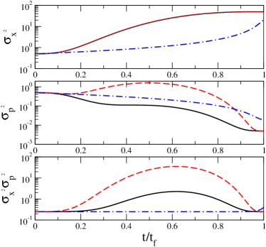
Figure 1: (Color online) Squeezing properties of the frictionless cooling strategies. Depicted is the time dependence of the position variance (top), momentum variance (center), and their product (bottom) for the three cooling strategies discussed in the text, with the product $\sigma_{x}^{2}\sigma_{p}^{2}$ expressed, from now on, in units of $\hbar^{2}$. The dashed and solid lines are for frictionless cooling with $t_{\mathrm{f}}$=6 ms and 25 ms, respectively. The dot-dashed line is for a linear ramp-down of the frequency corresponding to a quasi-adiabatic expansion occurring in a time $t_{\mathrm{f}}=2\pi/\omega_{\mathrm{f}}$ as discussed in Choi . The adiabatic invariant strategies allow for the preservation of states with minimal uncertainty product, as they display an uncertainty product returning to the value $\sigma_{x}^{2}\sigma_{p}^{2}=\hbar^{2}/4$ at $t=t_{\mathrm{f}}$ after a transient increase at earlier times. Conversely, the quasi-adiabatic expansion keeps its uncertainty product constant for a long time interval, but manifests an increase approaching the final time as the quasi-adiabaticity condition is less satisfied in the latest stage with minimal trapping frequency.

We show in Fig. 1 the time dependence of the position and momentum variances as well as their product for the two durations of cooling. The temporal variation of the position variance is found to be independent of $t_{\mathrm{f}}$, as expected from the analytical results, while the time evolution of the product of variances clearly indicates the recovery of the minimum uncertainty state at $t=t_{\mathrm{f}}$. For comparison, a quasi-adiabatic trajectory obtained by a linear ramping down of the frequency to its final value is also depicted, showing that the uncertainty product in this case exceeds the minimum value at final time.

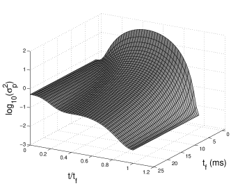
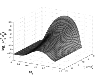
Figure 2: Top: $\log_{10}\sigma^{2}_{p}(t)$ calculated directly from the squeezing transformation for various $t_{\mathrm{f}}$. Bottom: $\log_{10}[\sigma^{2}_{x}(t)\sigma^{2}_{p}(t)]$ for various $t_{\mathrm{f}}$ indicating the deviation from, and the eventual return to, the minimum uncertainty state over time. It is noted that for small $t_{\mathrm{f}}$, the momentum variance $\sigma^{2}_{p}(t)$ proportional to the temperature, goes up significantly during the run. As previously noticed in our work Choi , due to potential atom loss, this presents a restriction on using this method in sympathetic cooling. A consequence relevant to this paper is the very high values of the product $\sigma^{2}_{x}(t)\sigma^{2}_{p}(t)$ during the run for short $t_{\mathrm{f}}$.

It should be noted here that, since Eqs. (5)-(7) are explicitly given in terms of the Ermakov solution $b(t)$, it is possible to directly calculate the amount of squeezing without evolving the wave function using the Schrödinger equation with a time-dependent potential. Figure 2 shows the momentum variance and the product of position and momentum variances as a function of time for various possible values of $t_{\mathrm{f}}$. The results for $t_{\mathrm{f}}$=6 ms and $t_{\mathrm{f}}$=25 ms obtained by evolving the Schrödinger equation, were found accurately reproduced. It is clear that the methods of quantum optical squeezing are applicable in the context of frictionless cooling, although the system is rather different from the standard quantum optical systems involving nonlinear optical media.

For small $t_{\mathrm{f}}$, it is noted that the momentum variance $\sigma^{2}_{p}(t)$ goes up significantly during the run, resulting in large values of the variance product, $\sigma^{2}_{x}(t)\sigma^{2}_{p}(t)$. The presence of such large deviation from the minimum uncertainty state during the run implies that, for such cases, any noise is likely to more effectively push the system away from the minimum uncertainty state. Indeed, we observe such a trend in the next section.

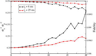
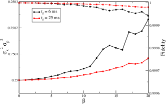
Figure 3: (Color online) The final variance product, $\sigma^{2}_{x}(t_{\mathrm{f}})\sigma^{2}_{p}(t_{\mathrm{f}})$ (bottom solid line, left vertical axis) and the fidelity (top dashed line, right vertical axis) for $t_{\mathrm{f}}$=25 ms (red squares) and $t_{\mathrm{f}}$=6 ms (black circles) as a function of noise amplitude $\beta$ described in the text. Gaussian white noise (top plot); uniform white noise (bottom plot), all from the averaging of 150 realizations.

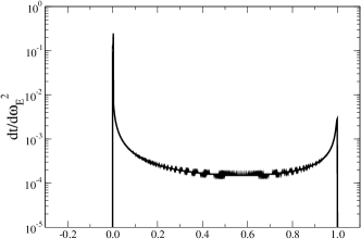
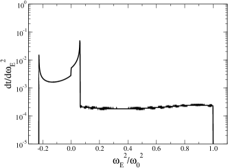
Figure 4: Temporal density of states versus $\omega^{2}/\omega_{0}^{2}$ for the two adiabatic strategies discussed in the text with $t_{\mathrm{f}}$=25 ms (top) and 6 ms (bottom). The temporal density of states, here evaluated for $10^{5}$ samples and $10^{3}$ squared frequency intervals in the entire range of variability of $\omega^{2}$, is normalized to unity, thereby representing the probability density to realize a given $\omega^{2}$ during the corresponding frictionless cooling process.

III Robustness of the frictionless cooling scheme

In this section, we want to answer the following question: how robust is the frictionless cooling technique to small deviations from the optimized Ermakov trajectory? Since, as discussed in the last section, the variable frequency strategy is basically mappable to a nonlinear system, the interplay between the deterministic Ermakov trajectory and any added noise may, in principle, be subtle and can lead to large and detrimental deviations from the idealized behavior. To study robustness in this system, we consider two experimentally relevant types of noise, broadband and monochromatic. These choices allow us to understand the system via the complementary responses.

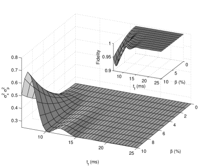
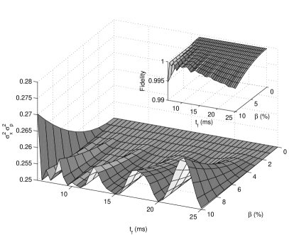
Figure 5: The final variance product, $\sigma^{2}_{x}(t_{\mathrm{f}})\sigma^{2}_{p}(t_{\mathrm{f}})$ and the fidelity (inset) as a function of $t_{\mathrm{f}}$ and the amplitude of sinusoidal modulation $\beta$ in a modulated trajectory $\omega^{2}_{s}(t)=\omega^{2}_{E}(t)[1+\beta\sin(\Omega_{n}t)]$. In the left panel we show the case of a sinusoidal noise within the range of trapping frequencies, $\Omega_{n}=\omega_{0}/2$, in the right panel an example of noise outside, $\Omega_{n}=3\omega_{0}/2$.

III.1 Response to random noise

For the random noise, we consider two different possibilities: Gaussian white noise with mean value $\omega^{2}_{E}(t)$, and standard deviation $\beta|\omega^{2}_{E}(t)|$, and uniformly distributed noise centered at $\omega^{2}_{E}(t)$ with width $\beta|\omega^{2}_{E}(t)|$, where $\beta$ is varied from zero to 0.2, i.e. in both situations noise has an amplitude up to 20% of the unperturbed trajectory $|\omega^{2}_{E}(t)|$. The results of simulations with the Gaussian white noise and uniform white noise are shown in Fig. 3 where the final variance product, $\sigma^{2}_{x}(t_{\mathrm{f}})\sigma^{2}_{p}(t_{\mathrm{f}})$ and the fidelity, obtained by averaging 150 trajectories, is depicted. Both the variance product and the fidelity show that the overall deviation from the desired result is of order $0.1\%$, and hence the system is relatively insensitive to random noise. This scheme is therefore more robust than we expected, especially given the very large amount of noise (up to 20%) added. This may be a result of the versatility of the Ermakov invariant scheme which, in principle, is able to handle all values of $t_{\mathrm{f}}$; the net effect of added noise may be viewed as shifting the final $t_{\mathrm{f}}$ which still produces the correct state. As expected, the final state deviates more and more from the desired state as one increases the noise amplitude $\beta$. It is worth noting that, as we had expected from examining Fig. 2, the $t_{\mathrm{f}}=$6 ms case with negative square frequency in the Ermakov trajectory is found to be more sensitive to the effect of noise. Physically, this is reasonable considering the added vulnerability to noise during the time interval in which atoms experience their antitrapping stage.

III.2 Response to sinusoidal modulation

Noting that realistic random noise can be viewed as a sum over sinusoidal modulations with random frequencies and amplitudes, one can analyze the robustness of this system by studying the response to a range of purely sinusoidal modulations. Sinusoidal modulations may occur as an unintended noise or added intentionally, for instance to improve the signal-to-noise ratio of a specific feature under investigation, to create arbitrary trapping potentials Courteille , or to prepare well-defined target states, for instance atomic Fock states in optical traps Dudarev ; Campo ; Pons ; Wan and optical lattices Meisner ; Nikolopoulos . Continuing our analogy to quantum optics, the study of monochromatic noise is similar to examining the response of a nonlinear optical medium to coherent light of fixed frequency.

Before such analysis we need to specify the range of trapping frequencies involved in the cooling procedure. We indeed expect that the effect of noise sources will depend on their relative location with respect to the spectrum of frequencies of the system. To quantify the latter, we introduce a ‘temporal’ density of states defined as the amount of time spent by the system in the range between $\omega^{2}_{E}$ and $\omega^{2}_{E}+d(\omega^{2}_{E})$. This is directly related, at least for monotonic decreases of the trapping frequency, to $[d(\omega^{2}_{E})/dt]^{-1}$, the inverse of the slope of the curve $\omega^{2}_{E}(t)$. For the case of nonmonotonic behavior, such as in the strategies involving a stage in which $\omega^{2}_{E}<0$, this is less trivial to obtain analytically. However, in practice, we can use a simple code in which we sort the times at which frequencies occur and count the number of times we find a square frequency in the $[\omega^{2}_{E},\omega^{2}_{E}+d(\omega^{2}_{E})]$ interval. For the frictionless cooling strategy with $t_{\mathrm{f}}$=25 ms this is depicted in the top plot of Fig. 4.

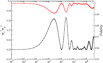
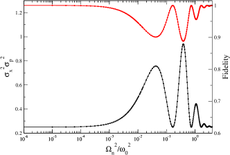
Figure 6: (Color online) The variance product, $\sigma^{2}_{x}(t_{\mathrm{f}})\sigma^{2}_{p}(t_{\mathrm{f}})$ (bottom solid line in black , left vertical axis) and the fidelity (top solid line in red , right vertical axis) as a function of the scaled modulation frequency $\Omega_{n}^{2}/\omega_{0}^{2}$ for fixed modulation amplitude $\beta=0.1$ with $t_{\mathrm{f}}$=25 ms (top plot) and $t_{\mathrm{f}}$=6 ms (bottom plot).

The case of strategies in which there are also time intervals with negative square frequencies is more involved, and a typical example is shown in the bottom plot of Fig. 4 for the $t_{\mathrm{f}}$=6 ms case. Multiple peaks now occur – one located at the minimum negative square frequency, as the system spends a large amount of time in that region, and another at a positive square frequency where the plot shows a local maximum in the final stage of cooling. The peak at zero frequency gets contributions from three distinct time intervals, two with a zero-crossing behavior, before and after reaching the minimum square frequency, and one from positive square frequencies alone at the very end of the cooling (see Fig. 1 in Choi ), resulting in a discontinuity in the temporal density of states. The high peaks in the $\omega^{2}<0$ region for the $t_{\mathrm{f}}=$6 ms case indicate that the contribution from the antitrapping stage is much more significant than what a simple inspection of the Ermakov trajectory would suggest.

The effect of sinusoidal noise was studied by modifying the Ermakov trajectory $\omega^{2}_{E}(t)$ to ${\tilde{\omega^{2}}_{E}(t)}=\omega^{2}_{E}(t)[1+\beta\sin(\Omega_{n}t)]$ and evolving the Schrödinger Equation under this time-dependent potential. In Fig. 5 we plot the final variance product, $\sigma^{2}_{x}(t_{\mathrm{f}})\sigma^{2}_{p}(t_{\mathrm{f}})$ and the fidelity (inset) for various $t_{\mathrm{f}}$ and $\beta$. We have chosen two possible cases of the modulation frequency, $\Omega_{n}<\omega_{0}$ ($\Omega_{n}=\omega_{0}/2$) and $\Omega_{n}>\omega_{0}$ ($\Omega_{n}=3\omega_{0}/2$). The results show that, as to be expected, the deviation from the desired state increases with increasing $\beta$, although the effect is now much more pronounced than those for the random noise. Again, as we expected from Fig. 2, it is seen that the short $t_{\mathrm{f}}$ cases that involve negative square frequencies are more sensitive to noise. There is also an overall oscillatory behavior as a function of $t_{\mathrm{f}}$ for the variance product, and this may be explained as follows. If one assumes, as a very crude, first order approximation, that the only relevant quantity in the wave function evolution is the instantaneous trapping frequency in the presence of noise, i.e. we completely disregard the trajectory history, one can write using Eq. (7) the final position variance

$$\sigma^{2}_{x}(t_{\mathrm{f}})\sigma^{2}_{p}(t_{\mathrm{f}})=\frac{\hbar^{2}}{4}\frac{\tilde{\omega}_{\mathrm{f}}}{\omega_{\mathrm{f}}},$$ (8)

where $\tilde{\omega}_{\mathrm{f}}$ is the new final trap frequency in the presence of the added noise. Given the form of the noise, we have $\tilde{\omega}_{\mathrm{f}}=\omega_{\mathrm{f}}\sqrt{1+\beta\sin(\Omega_{n}t_{\mathrm{f}})}$, and hence

$$\sigma^{2}_{x}(t_{\mathrm{f}})\sigma^{2}_{p}(t_{\mathrm{f}})\sim\frac{\hbar^{2}}{4}\sqrt{1+\beta\sin(\Omega_{n}t_{\mathrm{f}})},$$ (9)

so that there is an oscillatory behavior expected for the variance product as a function of $t_{\mathrm{f}}$ at constant $\Omega_{n}$ (and vice versa). This result indicates a fairly strong dependence of robustness on $t_{\mathrm{f}}$ or, to be more precise, on the deviation from the desired final trap frequency due to the presence of noise which, in this case, is given by the multiplicative factor $\sqrt{1+\beta\sin(\Omega_{n}t_{\mathrm{f}})}$.

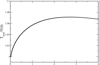
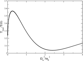
Figure 7: Scaled maximum temperature as a function of the the scaled modulation frequency $(\Omega_{n}^{2}/\omega_{0}^{2})$ for fixed modulation amplitude $\beta=10\%$ with $t_{\mathrm{f}}$=25 ms (top) and $t_{\mathrm{f}}$=6 ms (bottom).

Next, we have fixed the amplitude of the sinusoidal noise $\beta$ to be 0.1 i.e. 10% of the instantaneous Ermakov trajectory $\omega^{2}_{E}(t)$, and calculated the response of the system to noise in a range of modulation frequencies, $\Omega_{n}\in[0,2\omega_{0}]$. This is presented in Fig. 6 for both the $t_{\mathrm{f}}$=25 ms and $t_{\mathrm{f}}$=6 ms cases. It is observed that the system is fairly sensitive to the variation of the modulation frequency, and it is also evident that the $t_{\mathrm{f}}$= 6 ms case with the negative square frequency stage shows a very strong deviation from the desired state. As before, this is likely due to the enhanced vulnerability to external modulation during the anti-trapping stage. The oscillatory behavior as a function of the modulation frequency $\Omega_{n}$ for fixed $t_{\mathrm{f}}$ may, again, be partially explained using Eq. (9). From the same equation, the maximum possible deviation from the desired state is expected to be of the order $\beta/2$. Since we use $\beta$= 0.1 for the maximum noise, this rough estimate holds for the $t_{\mathrm{f}}$=25 ms case but not for the $t_{\mathrm{f}}$=6 ms case. The fact that the maximum possible deviation in variance product worked out from Eq. (9) is smaller than that observed indicates the presence of other contributing factors that disrupts the shortcut to adiabaticity as one would expect.

In order to produce a strong response, the modulation frequency $\Omega_{n}$ should, in general, match those trap frequencies along the trajectory that varies slowly i.e. those with large $dt/d(\omega^{2})$ in Fig. 4. For $t_{\mathrm{f}}$ = 25 ms this seems to be the case, in that the strongest response appears near $\Omega_{n}\approx 0$. However for $t_{\mathrm{f}}$ = 6 ms, although a strong response is also visible near the expected region of $\Omega_{n}\approx 0$, the maximum peak clearly appears near $\Omega_{n}^{2}/\omega_{0}^{2}\approx 0.5$. On close examination, it was found that the peaks appear near certain multiples of a characteristic angular frequency $\omega_{C}=\pi/2t_{\mathrm{f}}$, obtainable from Eq. (9) as the first local maximum. It was observed that the the first three peaks are found at $\tilde{\Omega}=\omega_{C}$, $4\omega_{C}$, and $7\omega_{C}$. Comparing the square of characteristic angular frequency, the $t_{\mathrm{f}}$ = 25 ms case gives $\tilde{\Omega}^{2}/\omega_{0}^{2}=0.0016,0.0256,0.0784$, while the $t_{\mathrm{f}}$ = 6 ms case gives $\tilde{\Omega}^{2}/\omega_{0}^{2}=0.0278,0.4444,1.3611$, approximately coinciding with the corresponding locations of the maximum peaks. This shows that, in addition to the temporal density of states, the characteristic angular frequency that depends on the precise type of noise and its effect on the final trapping frequency is another important parameter in characterizing the robustness of this system.

Finally, we note that the overall behavior of the fidelity mirrors that of the variance product, indicating that, in our case, the amount of squeezing is indeed an efficient alternative parametrization of robustness.

III.3 Reduction of the maximum temperature

A crucial finding in our previous work Choi was the limitation imposed by the high temperature attained by the atoms during the cooling process. Therefore, related to the study of robustness of the system to noise, we have investigated the maximum temperature attained by the atoms during the cooling process in the presence of sinusoidal modulation of various modulation frequencies. For the Ermakov trajectory which does not contain an antitrapping stage, the sinusoidal modulation can provide momentum kicks, increasing the momentum variance. On the other hand, for the $t_{\mathrm{f}}$=6 ms case that includes an antitrapping stage, with a modulation of the curvature of the anti-trap one may be able to “catch” the wave function spread in such a way that the momentum variance is reduced. Qualitatively, this may be viewed similarly to the mechanism behind the dynamic equilibrium attained by an inverted pendulum with an oscillating pivot. Figure 7 shows the scaled maximum temperature as a function of the modulation frequency. It is found that for the $t_{\mathrm{f}}$=25 ms case, there is some heating as the modulation frequency is increased. However, interestingly, for the $t_{\mathrm{f}}=$6 ms case that contains the negative square frequency stage, it shows a dip in the maximum temperature around the modulation frequency of $\Omega_{n}=1.55\omega_{0}$ to a value less than that corresponding to no sinusoidal modulation ($\Omega_{n}=0$). In addition, the variance product at this frequency is also very close to the minimum uncertainty state, indicating this is the optimum set-up for the $t_{\mathrm{f}}$= 6 ms case if reducing atom losses is the most important priority. This provides a motivation for intentionally adding a sinusoidal modulation in the cooling scheme to minimize atom-loss due to heating, adding a further dimension to the issue of cooling optimization when an antitrapping stage is present Stefanatos . It has been shown Stefanatos1 that the cooling time is minimized, in the presence of a trapping stage, using a “bang-bang” control, i.e. with stepwise changes of the trapping frequency, but the possible addition of a sinusoidal driving may call for a modification, or at least a check, of this optimization procedure.

IV Discussion

The results reported in this paper are encouraging for the experimental implementation of frictionless cooling, possibly including a negative square frequency stage, in Fermi-Bose mixtures using optical dipole traps and optical lattices. A scheme using a single-frequency optical dipole trap with a continuously tunable laser is not feasible due to the large atom losses expected in crossing the dominant atomic transition from the red-detuned to the blue-detuned side to achieve antitrapping. Nevertheless, this issue may be circumvented through the use of two laser beams at constant frequencies, opposite detunings, and variable power ratio, such as the bichromatic optical dipole traps proposed in Onofrio to allow optimal heat capacity matching between the Bose and Fermi gases Presilla ; JSP . The presence of noise related to power fluctuations and beam-pointing stability for both laser beams in this configuration makes the discussion presented in this paper quite relevant for implementing frictionless cooling in bichromatic optical dipole traps. Bichromatic trapping has been recently implemented at the magneto-optical trap stage for a single species Qiang , and two-species selective trapping and cooling has been demonstrated with hybrid traps involving magnetic and optical confinement Catani ; Baumer . Therefore experiments involving trapping and cooling of two species in a bichromatic trap should be within reach in the near future. Our discussion should also be relevant to the case of frictionless cooling in optical lattices, as recently discussed Yuce1 . Dynamically variable spacing (the so-called accordion lattice) allows for a continuous increase of lattice periodicity, as experimentally demonstrated in Fallani ; Li ; Assam , without the need to change the laser frequency. In this case an additional source of noise during the trap expansion is due to the presence of acousto-optic deflectors, adding up to the beam-pointing stability of the lasers. Implementing frictionless cooling with a negative square frequency stage via a bichromatic optical lattice could also be of great relevance to investigate fundamental issues of statistical mechanics as the approach to equilibrium in atomic systems at negative temperatures Mosk ; Rapp ; Iubini .

In summary, we have found that the robustness of the frictionless cooling method to noise can be analyzed by characterizing the final quantum state in terms of the amount of squeezing as well as the usual fidelity. It was found that the method is quite robust to the presence of broadband noise in the trapping frequency, and further analysis involving monochromatic sinusoidal modulation has allowed us to resolve its response. We have studied the dependence of the squeezing and fidelity on the deviation from the expected Ermakov trajectory, and identified the role of such measures as the temporal density of states and characteristic angular frequency. Numerical simulations indicate that, despite the perception that short $t_{\mathrm{f}}$ could mean less time for noise to interfere with the system, too short a $t_{\mathrm{f}}$ is best avoided in practice. In addition, a way to reduce the maximum temperature and hence atom losses was found by adding a high frequency sinusoidal modulation, which helps to mitigate one of the limitations of this scheme found in our previous work.

References

- (1) X. Chen, A. Ruschhaupt, S. Schmidt, A. del Campo, D. Guéry-Odelin, and J. G. Muga, Phys. Rev. Lett. 104, 063002 (2010).
- (2) J.-F. Schaff, X.-L. Song, P. Vignolo, and G. Labeyrie, Phys. Rev. A 82, 033430 (2010).
- (3) J.-F. Schaff, X.-L. Song, P. Capuzzi, P. Vignolo, and G. Labeyrie, EPL 93, 23001 (2011).
- (4) E. Torrontegui, S. Ibàñez, X. Chen, A. Ruschhaupt, D. Guéry-Odelin, and J. G. Muga, Phys. Rev. A 83, 013415 (2011).
- (5) X. Chen and J. G. Muga, Phys. Rev. A 82, 053403 (2010).
- (6) E. Torrontegui, X. Chen, M. Modugno, A. Ruschhaupt, D. Guéry-Odelin, and J. G. Muga, Phys. Rev. A 85, 033605 (2012).
- (7) S. Choi, R. Onofrio, and B. Sundaram, Phys. Rev. A 84, 051601(R) (2011).
- (8) M. J. Davis, P. B. Blakie, A. H. van Amerongen, N. J. van Druten, and K. V. Kheruntsyan, Phys. Rev. A 85, 031604 (2012).
- (9) H. R. Lewis, Phys. Rev. Lett. 18, 510 (1967).
- (10) H. R. Lewis and W. B. Riesenfeld, J. Math. Phys. (N.Y.) 10, 1458 (1969).
- (11) D. Sokolovski, M. Pons, A. del Campo, and J. G. Muga, Phys. Rev. A 83, 013402 (2011).
- (12) D. F. Walls and G. J. Milburn, Quantum Optics (Springer-Verlag, Berlin, 1994); S. M. Barnett and P. M. Radmore, Methods in Theoretical Quantum Optics (Oxford University Press, New York, 2002).
- (13) C. Yuce, A. Kilic, and A. Coruh, Phys. Scr. 74, 114 (2006).
- (14) Ph. W. Courteille, B. Deh, J. Fortágh, A. Günther, S. Kraft, C. Marzok, S. Slama, and C. Zimmermann, J. Phys. B 39, 1055 (2006).
- (15) A. M. Dudarev, M. G. Raizen, and Q. Niu, Phys. Rev. Lett. 98, 063001 (2007).
- (16) A. del Campo and J. G. Muga, Phys. Rev. A 78, 023412 (2008).
- (17) M. Pons, A. del Campo, J. G. Muga, and M. G. Raizen, Phys. Rev. A 79, 033629 (2009).
- (18) S. Wan, M. G. Raizen, and Q. Niu, J. Phys. B 42, 195506 (2009).
- (19) M. G. Raizen, S. P. Wan, C. Zhang, and Q. Niu, Phys. Rev. A 80, 030302(R) (2009).
- (20) F. Heidrich-Meisner, S. R. Manmana, M. Rigol, A. Muramatsu, A. E. Feiguin, and E. Dagotto, Phys. Rev. A 80, 041603(R) (2009).
- (21) G. M. Nikolopoulos and D. Petrosyan, J. Phys. B 43, 131001 (2010).
- (22) D. Stefanatos, H. Schaettler, and J.-S. Li, SIAM J. Control Optim. 89, 2440 (2011).
- (23) D. Stefanatos, J. Ruths, and J.-S. Li, Phys. Rev. A 82, 063422 (2010).
- (24) R. Onofrio and C. Presilla, Phys. Rev. Lett. 89, 100401 (2002).
- (25) C. Presilla and R. Onofrio, Phys. Rev. Lett. 90, 030404 (2003).
- (26) R. Onofrio and C. Presilla, J. Stat. Phys. 115, 57 (2004).
- (27) C. Qiang, L. Xin-Yu, G. Kui-Yi, W. Xiao-Rui, C. Dong-Min, and W. Ru-Quan, Chin. Phys. B 21, 043203 (2012).
- (28) J. Catani, G. Barontini, G. Lamporesi, F. Rabatti, G. Thalhammer, F. Minardi, S. Stringari, and M. Inguscio, Phys. Rev. Lett. 103, 140401 (2009).
- (29) F. Baumer, F. Münchow, A. Görlitz, S. E. Maxwell, P. S. Julienne, and E. Tiesinga, Phys. Rev. A 83, 040702(R) (2011).
- (30) C. Yuce, Phys. Lett. A 376, 1717 (2012).
- (31) L. Fallani, C. Fort, J. E. Lye, and M. Inguscio, Optics Express 13, 4303 (2005).
- (32) T. C. Li, H. Kelkar, D. Medellin, and M. G. Raizen, Optics Express 19, 5465 (2008).
- (33) S. Al-Assam, R. A. Williams, and C. J. Foot, Phys. Rev. A 82, 021604(R) (2010).
- (34) A. P. Mosk, Phys. Rev. Lett. 95, 040403 (2005).
- (35) A. Rapp, S. Mandt, and A. Rosch, Phys. Rev. Lett. 105, 220405 (2010).
- (36) S. Iubini, R. Franzosi, R. Livi, G.-L. Oppo, and A. Politi, arXiv:1203.4162 (19 Mar 2012).