Globular Cluster Systems of Spiral and S0 Galaxies:
Results from WIYN Imaging of NGC 1023, NGC 1055, NGC 7332 and NGC 7339

Abstract

We present results from a study of the globular cluster (GC) systems of four spiral and S0 galaxies imaged as part of an ongoing wide-field survey of the GC systems of giant galaxies. The target galaxies — the SB0 galaxy NGC 1023, the SBb galaxy NGC 1055, and an isolated pair comprised of the Sbc galaxy NGC 7339 and the S0 galaxy NGC 7332 — were observed in $BVR$ filters with the WIYN 3.5-m telescope and Minimosaic camera. For two of the galaxies, we combined the WIYN imaging with previously-published data from the Hubble Space Telescope and the Keck Observatory to help characterize the GC distribution in the central few kiloparsecs. We determine the radial distribution (surface density of GCs versus projected radius) of each galaxy’s GC system and use it to calculate the total number of GCs ($N_{GC}$). We find $N_{GC}$ $=$ $490\pm 30$, $210\pm 40$, $175\pm 15$, and $75\pm 10$ for NGC 1023, NGC 1055, NGC 7332, and NGC 7339, respectively. We also calculate the GC specific frequency ($N_{GC}$ normalized by host galaxy luminosity or mass) and find values typical of those of the other spiral and E/S0 galaxies in the survey. The two lenticular galaxies have sufficient numbers of GC candidates for us to perform statistical tests for bimodality in the GC color distributions. We find evidence at a high confidence level ($>$95%) for two populations in the $B-R$ distribution of the GC system of NGC 1023. We find weaker evidence for bimodality ($>$81% confidence) in the GC color distribution of NGC 7332. Finally, we identify eight GC candidates that may be associated with the Magellanic dwarf galaxy NGC 1023A, a satellite of NGC 1023.

1. Introduction

Studies of the spatial distribution, metallicities, and kinematics of the globular clusters (GCs) in the Milky Way have provided us with fundamental insights into the formation and evolutionary history of our own Galaxy (e.g., Searle & Zinn 1978, Zinn 1985, Armandroff & Zinn 1988, Zinn 1993, Mackey & van den Bergh 2005). This link exists more generally as well: studies of GCs in other giant galaxies can provide us with clues to the host galaxies’ origins and structure. These luminous, old star clusters seem to mark the major star formation and merger episodes in galaxies (e.g., Schweizer 1987, Whitmore et al. 1993, Whitmore & Schweizer 1995, Brodie & Strader 2006 and references therein) as well as acting as kinematic and dynamical tracers of the outer regions of galaxies, which are difficult to probe via integrated light (e.g., Zepf et al. 2000, Côté et al. 2001, Richtler et al. 2004, Bridges et al. 2007, Strader et al. 2011).

Steady progress has been made in our understanding of extragalactic GC systems in the $\sim$20 years since Harris’ 1991 comprehensive annual review of GC systems in galaxies beyond the Local Group. Many of the major advances in extragalactic GC system research were made possible by the Hubble Space Telescope (HST): for example, HST has enabled systematic surveys of the GC systems of hundreds of galaxies in the (relatively nearby) Virgo and Fornax clusters (Côté et al. 2004, Jordán et al. 2007) as well as detection of GCs in galaxy clusters $>$100 Mpc away (e.g., West et al. 2011). Nevertheless one of the deficiencies pointed out in both the book on globular cluster systems by Ashman & Zepf (1998) and the Annual Review by Brodie & Strader (2006) is the relative rarity of wide-field CCD studies that are able to measure accurate global properties of giant galaxy GC populations. Reliable measurements of quantities like the spatial distribution of the GC system, the total number of GCs, the GC specific frequency, and the global color distribution require wide-field CCD imaging in multiple filters. A CCD camera with a field-of-view (FOV) many arc minutes on a side is needed to cover the full radial extent of the GC systems of galaxies within $\sim$20$-$30 Mpc and accurate multi-color photometry is crucial for minimizing contamination from non-GCs (e.g., Rhode & Zepf 2001, Dirsch et al. 2003).

Our group is engaged in an ongoing survey aimed at quantifying the global properties of the GC populations of giant galaxies. We use multi-color imaging with mosaic CCD cameras and target giant spiral, S0, and elliptical galaxies at distances between $\sim$10$-$25 Mpc. To date we have observed $>$30 giant galaxies with a range of masses, morphological types, and luminosities; results for the galaxies we have finished analyzing are published in a series of papers (Rhode & Zepf 2001, 2003, 2004; Rhode et al. 2005, 2007, 2010, Hargis et al. 2011; hereafter RZ01, RZ03, RZ04, R05, R07, R10, H11). Other groups who use multi-color wide-field imaging techniques have for the most part targeted massive elliptical galaxies with very populous, extended GC systems (e.g., Dirsch et al. 2003, imaging of NGC 1399; Tamura et al. 2006, imaging of M87; Dirsch et al. 2005, imaging of NGC 4636). We have recently observed a number of moderate-luminosity spiral and S0 galaxies in order to fill in specific gaps in our survey and in the general census of giant galaxies that have been imaged with wide-field CCD cameras. Furthermore, these galaxies are a good match, in terms of their observational requirements, for the FOV and sensitivity of the WIYN 3.5-m telescope and Minimosaic imager.

In this paper we present results from WIYN Minimosaic imaging of the GC populations of four moderate-luminosity spiral and lenticular galaxies: the SB0 galaxy NGC 1023, the SBb galaxy NGC 1055, and the isolated S0/Sbc galaxy pair NGC 7332 and NGC 7339. Basic properties of the four galaxies — morphological type, distance, absolute magnitude, stellar mass, and environment — are listed in Table 1. The GC systems of two of the galaxies, NGC 1023 and NGC 7332, were studied by Larsen & Brodie (2000) and Forbes et al. (2001), respectively, so we have combined their previous results with our wide-field data to produce the full GC system radial distributions for those two galaxies. Also included in our WIYN imaging of NGC 1023 is the Magellanic dwarf galaxy NGC 1023A, so we identify a subsample of GC candidates that may be associated with NGC 1023A and estimate this galaxy’s total GC population and specific frequency.

The paper is laid out as follows. The next two sections describe the data acquisition and image reductions (Section 2) and the detection and selection of GC candidates around each galaxy (Section 3). Section 4 addresses the issues of completeness and contamination in the GC candidate samples. The results of the analysis — including the radial profiles of each galaxy’s GC system, the total number and specific frequency of GCs, and analysis of the GC color distributions — are presented in Section 5. The last section of the paper gives a brief summary of the main conclusions.

2. Observations & Image Reductions

Images of the target galaxies were obtained in September 2008 and September 2009 at Kitt Peak National Observatory with the 3.5 m WIYN telescope and Minimosaic camera. The detector is comprised of two 2048 $\times$ 4096 CCDs with 0.141^′′ pixels, and a FOV of 9.6^′ $\times$ 9.6^′ when paired with the WIYN telescope. The relatively large FOV allowed us to image the isolated galaxy pair NGC 7332 and NGC 7339 simultaneously. To obtain sufficient radial coverage of these galaxies’ GC systems, NGC 7339 was positioned near the top center of the field, while NGC 7332 was placed in the lower right. NGC 1023 and 1055 were both positioned in the center of one CCD (away from a narrow gap between the two Minimosaic CCDs). Figures 1-3 show the WIYN FOV for each target galaxy overlaid on a Digitized Sky Survey (DSS)  image. To help us differentiate GCs from contaminating foreground stars and background galaxies, multiple exposures were taken in each of three broadband filters ($BVR$). For a list of exposure times see Table 2.

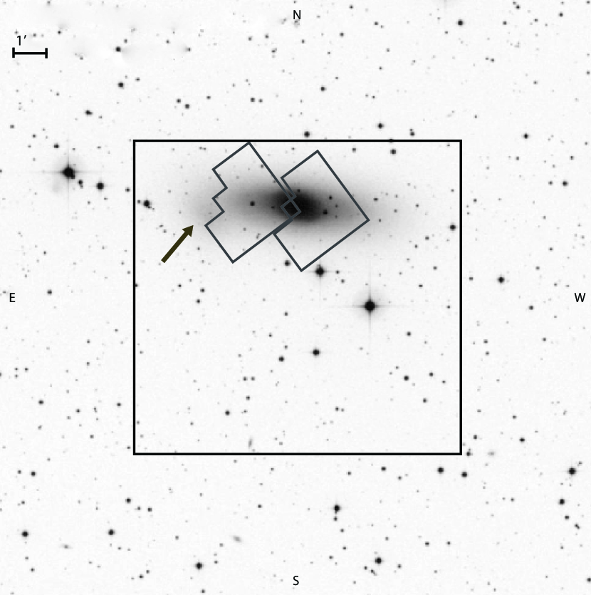
Figure 1.— Digitized Sky Survey image of the S0 galaxy NGC 1023 with the location of the WIYN Minimosaic pointing indicated by the large box. The locations of two HST WFPC2 pointings that were first analyzed by Larsen & Brodie (2000) and which are discussed in Section 5.2 are overlaid on the central portion of the galaxy. The location of the dwarf galaxy NGC 1023A (discussed in Section 5.5) is marked with an arrow.

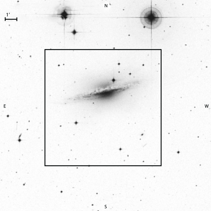
Figure 2.— Digitized Sky Survey image of the Sb spiral galaxy NGC 1055 with the location of the WIYN Minimosaic pointing indicated by a large box.

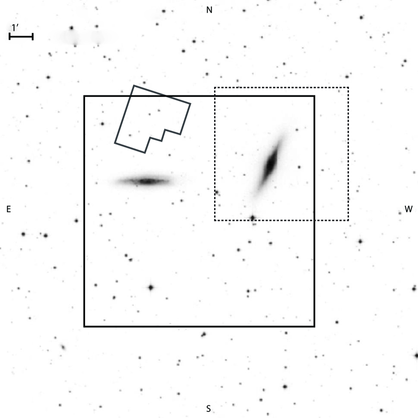
Figure 3.— Digitized Sky Survey image of the S0 peculiar galaxy NGC 7332 (right) and the Sbc spiral galaxy NGC 7339 (left) with the location of the WIYN Minimosaic pointing indicated by a large box. The HST WFPC2 pointing discussed in Section 4.2.2 is marked just north of NGC 7339. The box marked with a dotted line around NGC 7332 marks the FOV of the Keck observation analyzed by Forbes et al. (2001) and discussed in Section 5.2.

Observations of photometric standard star fields (Landolt, 1992) were made in photometric conditions throughout the first night of the 2008 observing run and the third night of the 2009 run, along with at least one exposure of each target galaxy in all three filters. These observations were used to determine the color terms and zero point constants for the data taken on the photometric nights. The calculated errors on the zero point constants were all less than or equal to 0.007 magnitude, which demonstrates that those nights were genuinely photometric.

Standard reductions (overscan and bias level subtraction, flat-field division) were performed on all of the Minimosaic images using tasks in the IRAF package MSCRED. The MSCRED tasks msczero, msccmatch, and mscimage were then used to convert the multi-extension FITS images into single-extension images. The images taken of a given target galaxy were aligned to each other. A constant sky background level was measured for each image and subtracted. Images of a given galaxy taken in the same filter were then scaled to a common flux level and combined using the IRAF task imcombine and the ccdclip pixel rejection algorithm. The constant sky background level was then added back to the final combined image. The result of this processing was a single deep, stacked image of each target galaxy in each filter. The mean full-width at half-maximum of the point-spread function (FWHM PSF) in the combined $BVR$ images ranged from $0.6{{}^{\prime\prime}}-1.0{{}^{\prime\prime}}$ for NGC 1023, $0.9{{}^{\prime\prime}}-1.0{{}^{\prime\prime}}$ for NGC 7332 & NGC 7339, and $1.0{{}^{\prime\prime}}-1.1{{}^{\prime\prime}}$ for NGC 1055. The method we used for calibrating the photometry in the final stacked images (using the data taken on the photometric nights of the 2008 and 2009 runs) is explained in Section 3.3.

3. Detection and Analysis of the Globular Cluster Systems

3.1. Source Detection

To facilitate detection of GC candidates close to each target galaxy, we executed a series of steps to remove the diffuse galaxy light from the deep, stacked images. We began by smoothing each of the images with a circular median filter with a diameter 7$-$7.5 times the mean FWHM PSF of the image. The size of the median filter was chosen after testing to find the optimal size for removing diffuse light from the galaxy while preserving the PSF of the compact, star-like objects around the galaxy. This smoothed image was then subtracted from the original version. A constant background level was added to the resultant images to preserve the photometric integrity of later measurements. The rest of the analysis steps were performed on these “galaxy-subtracted” images (one such image for each filter and each galaxy field).

Some regions of the galaxy-subtracted images — such as small areas around saturated stars and high-background areas in the galaxy disks — were masked out prior to the detection step in order to minimize spurious detections. The IRAF task daofind was then used to identify sources above a given signal-to-noise threshold in each image. The source lists for the $B$, $V$, and $R$ filters were matched, and only sources that appeared in all three filters were retained in the final list of detected objects for a particular galaxy field. For NGC 7332 & NGC 7339 a total of 1126 objects appeared in all three filters, while NGC 1055 had 343 matched objects and NGC 1023 had 2141 matched objects. The relatively small numbers of objects found in the NGC 1055 field compared to the other two fields had two causes. First, NGC 1055 has a higher Galactic latitude than the other galaxy fields — its latitude is $b$ $=$ $-$51 degrees, compared to $b$ $=$ $-$19 degrees for NGC 1023 and $b$ $=$ $-$29 degrees for NGC 7332 — so many fewer Galactic foreground stars appear in the NGC 1055 field. Secondly, NGC 1055 is an Sb spiral galaxy, whereas NGC 1023 and NGC 7332 are S0 galaxies; we are finding in our GC system survey that spiral galaxies typically have many fewer GC candidates around them than early-type galaxies.

3.2. Removing Extended Sources

Given the distances to the target galaxies ($\sim$10$-$20 Mpc; see Table 1), GCs should appear as unresolved point sources in our ground-based images. The median half-light radius for Milky Way GCs is 3 pc (Ashman & Zepf, 1998), which subtends 0.06^′′ at 10 Mpc, and our images have FWHM PSF values of 0.6$-$1.1^′′. Thus any extended objects are not real GCs and need to be removed from the source lists. To accomplish this, we plotted the FWHM of the detected objects against instrumental magnitude (separately for each galaxy field and for each filter). In such a diagram, point sources produce a tight grouping that flares at faint magnitudes. Sources that deviated markedly from this sequence in any of the three filters were eliminated from the source list. Our extended source cut for NGC 1023 is illustrated in Figure 4; a similar cut was applied to all three target fields. Once the extended objects were removed, the source list for NGC 1023 contained 917 objects. The source list for NGC 1055 included 257 objects, and the list for NGC 7332/NGC 7339 had 642 objects.

Figure 4.— An example of the extended source cut step: the plots show measured FWHM vs instrumental $B$, $V$, and $R$ magnitude in the final combined images of NGC 1023. Filled circles mark the 917 objects that passed the extended source cut in all three filters. Open squares mark rejected objects. Similar cuts were applied to the source lists for all target galaxies.

3.3. Aperture Photometry of Matched Point Sources

Calibrated $B$, $V$, and $R$ magnitudes for the matched list of point sources in each galaxy field were derived using the following procedure. Aperture photometry was performed on the point sources in each field (i.e., the 917 sources in the NGC 1023 field, the 257 objects in the NGC 1055 field, and the 642 objects in the NGC 7332/NGC 7339 field) using the IRAF task PHOT. The radii of the apertures used to do the photometry were set equal to the mean FWHM value of the image. An aperture correction was derived for each image by calculating the mean of the difference between the total magnitude and the magnitude measured within a one-FWHM-radius aperture for a set of $\sim$10$-$20 bright point sources.

In addition to the aperture correction, a bootstrap correction was determined for calibrating our stacked images, which are a combination of images taken on both photometric and non-photometric nights. To calculate the bootstrap correction, instrumental magnitudes of bright objects were compared between single-frame images taken on photometric nights and the final stacked images of a given target field. The mean magnitude difference between the single photometric image and the final, combined image was calculated for each case. We also determined foreground Galactic extinction corrections (in the direction of each target galaxy field) from the maps of infrared dust emission presented in Schlegel et al. (1998).

Total instrumental magnitudes were calculated for the matched point sources by applying the appropriate aperture, bootstrap, and airmass corrections to the instrumental magnitudes measured with the one-FWHM-radius aperture. These magnitudes were then calibrated using the appropriate photometric coefficients and Galactic extinction corrections, to produce final $B_{0}$, $V_{0}$, and $R_{0}$ magnitudes and colors for the point sources.

3.4. Final Selection of GC Candidates

In the final GC candidate selection step, we establish an expected range of $BVR$ magnitudes and colors for GCs at the target galaxies’ distances and keep only the objects that are consistent with those values. The GC luminosity function (GCLF) of the Milky Way and other giant galaxies indicates that the most luminous GCs will typically have $M_{V}$ $\sim$ $-$11 (Ashman & Zepf, 1998). For NGC 1055, we eliminated point sources with $M_{V}$ brighter than $-$11 (assuming the distance modulus given in Table 1). For NGC 7332 and NGC 7339, there were three point sources that were close to the host galaxies, looked like GCs, and had $M_{V}$ values a few tenths of a magnitude brighter than $-$11. We relaxed the bright-end magnitude criterion slightly in order to include only these three specific objects. In the case of NGC 1023, we adjusted our bright-end cut to include a luminous, spectroscopically-confirmed GC originally identified by Larsen & Brodie (2000). Relaxing the bright-magnitude criterion yielded an extra seven objects around NGC 1023 that have GC-like colors and $M_{V}$ magnitudes brighter than $-$11. The sequence numbers, positions, $V$ magnitudes, and $B-V$ and $V-R$ colors and corresponding errors for these seven objects are given in Table 3. Given our assumed distance modulus for NGC 1023 ($m-M$$=$30.29), the $M_{V}$ values for these seven objects range from $-$11.4 to $-$11.0. (We note that two of the objects, 119 and 133, are located several arc minutes away from the galaxy center and thus would seem less likely than the objects at small projected radial distances to be bona fide GCs.) For the NGC 7332/7339 field we also implemented a faint source cut, eliminating objects with $V>24.4$. We did this to remove a number of faint objects that had large magnitude errors (${}_{>}\atop{{}^{\sim}}$0.15) and were located many arc minutes from the target galaxy; these are likely to be unresolved background galaxies. For similar reasons a faint cut of $V>23.5$ was implemented for both the NGC 1023 and NGC 1055 fields. (Note that any GCs we miss due to the magnitude incompleteness of our images and the cuts imposed on the samples at the faint end are accounted for in the GCLF correction step described in Section 4.3.)

We also implemented the standard $BVR$ color selection that we use for the wide-field survey (see Rhode & Zepf, 2001 for more details): we removed point sources that lie more than $3\sigma$ away from the mean $V-R$ vs. $B-V$ relation for Galactic GCs with metallicities between [Fe/H] of $-2.5$ and $0.0$. When we test whether each source is consistent within $3\sigma$ of the Milky Way GC color-color relation, we take into account the object’s photometric error. For NGC 7332 we added a single object that fell just barely outside the color criteria and was located close ( $<0.4$^′) to the galaxy center.

GC candidates positioned very close to the host galaxy disk may be subject to additional reddening and thus might appear in the $BVR$ color-color diagram just redward of the GC candidate selection box. Point sources that appeared in this part of the color-color diagram were individually examined in the images. For all four of the target galaxies, none of the objects just redward of the color selection box were positioned close to the host galaxy disk in the images, so we did not add any such candidates to our final list.

An additional complicating factor in the detection of GC candidates around NGC 1023 was the presence of the dwarf galaxy NGC 1023A. The galaxy is classified as a Magellanic irregular in RC3 (de Vaucouleurs et al., 1991) and is located $\sim$2.5^′ (a projected distance of $\sim$8 kpc) to the southeast of NGC 1023 in the image. According to the NASA Extragalactic Database (NED), NGC 1023A is a member of the NGC 1023 group. We determined that the light from NGC 1023A extends over a circular region with a radius of 0.6^′ in the $V$-band image. We did this by plotting the pixel intensities along the radial direction between NGC 1023A and NGC 1023 to find the radial distance at which the light from NGC 1023A begins to dominate. We measured this radial distance in all three of the combined images and averaged the results to come up with the radial size of NGC 1023A in the images. We excluded this region from the rest of our analysis of NGC 1023’s GC system. Eight of the point sources with magnitudes and colors like GCs are located within that circular region. We note that, without additional information, we cannot definitively say with which galaxy these objects are associated. We explore the properties of these eight objects in further depth in Section 5.5, including estimating how many of them are likely to be GCs in the dwarf galaxy (rather than part of NGC 1023’s GC system). We correct for the area that was masked around NGC 1023A when we construct the radial profile for NGC 1023’s GC system (see Section 5.1).

The final GC candidate list for NGC 1023 contained 192 objects, while NGC 1055 had 60 GC candidates and NGC 7732 and NGC 7339 together had 105 GC candidates. Figures 5 — 7 show the $BVR$ color-color diagrams for the point sources detected around the four galaxies. Open squares represent the detected point sources, and the filled circles show the objects that were selected for the final GC candidate list. The GC color selection box and the mean $V-R$ vs. $B-V$ relation for Milky Way GCs (the line marking the midpoint of the box) are marked with solid lines. The tracks indicate the expected colors for galaxies of different morphological types at redshifts between $z=0$ and $z=0.7$, to illustrate possible sources of background galaxy contamination; i.e., to show what types of galaxies, and at what redshifts, are likely to lie in the same part of the $BVR$ color-color plane as GCs. (See RZ01 for a full discussion of how the color cut for the survey was developed and details about how these galaxy tracks were produced.)

Figure 5.— Selection of GC candidates in NGC 1023 based on $V-R$ and $B-V$ colors and $V$ magnitudes. The 917 point sources that survived the extended source cut in all three filters are marked with open squares. The final selected 192 GC candidates are indicated with filled circles. The box marks the area of our color selection. Sources outside the color selection area, but with colors and corresponding errors consistent with the selection criteria are retained as GC candidates. A reddening vector equivalent to $A_{V}$ = $1$ is in the lower right-hand corner of the image. The curves mark the colors of galaxies of several morphological types in a redshift range of z = 0 to z = 0.7, indicating possible sources of background contamination (see Rhode & Zepf 2001 for details of how the curves were generated).

Figure 6.— Selection of GC candidates in NGC 1055 based on $V-R$ and $B-V$ colors and $V$ magnitudes, plotted in the same way as in Figure 5. The 257 point sources that passed the extended source cut in all three filters are marked with open squares; the 60 GC candidates are marked with open circles.

Figure 7.— Selection of GC candidates in both NGC 7332 and NGC 7339 based on $V-R$ and $B-V$ colors and $V$ magnitudes, plotted in the same way as in Figure 5. These galaxies were included in the same image so the GC selection was done over the full field, for both galaxies at once. The 642 point sources that survived the extended source cut in all three filters are marked with open squares; the 105 GC candidates in the NGC 7332/NGC 7339 field are marked with filled circles.

4. Additional Analysis Steps

4.1. Completeness Testing and Detection Limits

In order to determine the limit of our ability to detect point sources of a given magnitude in the galaxy-subtracted images, we created a series of tests to quantify the completeness level as a function of object magnitude in each filter for each galaxy field. We first measured the typical PSF for each image. We added 200 artificial point sources with the appropriate PSF and a given magnitude to each of the combined images ($B$, $V$, and $R$). We did this in 0.2-magnitude steps over a range of 6$-$7 magnitudes, creating a separate image for each magnitude step (and each filter). The images with the artificial point sources were then processed in a series of steps identical to the detection steps we had executed to find GC candidates in the original images. For each magnitude step and each filter, we determined what fraction of the artificial sources were recovered. This gave us an estimate of the completeness at that magnitude, i.e., our ability to detect point sources of a given magnitude in a given image. The result was a series of completeness curves, one for each filter, for each set of galaxy-subtracted combined images. The completeness information was taken into account in our analysis of what fraction of the GC luminosity function we had covered for each galaxy (see Section 4.3). The 50% completeness limits are typically $\sim 24$-$25$ magnitudes; Table 4 lists the exact values for each image.

4.2. Contamination

Contamination of the GC candidate lists by foreground stars and background compact galaxies occurs because some of these objects may match all of the selection criteria for GC candidates. Here we present our methods for quantifying the contamination level and, where possible, correcting for the presence of contaminating objects.

4.2.1 Model Prediction for Stellar Contamination

We used a Galactic stellar population synthesis model to estimate the level of stellar foreground contamination that might be present in the GC candidate lists. Hereafter we refer to the model as the Besançon model; a complete description of the model and the observational constraints used to develop it are given in Robin et al. (2003). Briefly, the model divides the Milky Way Galaxy into four distinct stellar populations: a thin disk, a thick disk, a spheroid, and a bulge. Each component is defined by a star formation rate, initial mass function, metallicity distribution, kinematics, and evolutionary tracks within the model. Given a range of stellar types, magnitudes, and colors, the model uses Monte Carlo methods to produce Galactic star counts for a specific region of the sky. Comparisons of the star count predictions of the Besançon model to photometric surveys have shown reasonable agreement (e.g., Robin et al., 2000 and Reyle & Robin, 2001).

We used the Besançon model to estimate the number of Galactic foreground stars that would appear within the fields of view of our Minimosaic pointings. In order to arrive at an estimate of the number of possible contaminants in the GC candidate samples, we set the inputs of the model to provide counts only for Galactic stars with $B-V$ colors, $V-R$ colors, and $V$ magnitudes defined by the range of properties in the final selected GC candidate list for each galaxy. To account for the statistical nature of the model, we ran it ten times per target galaxy field and then calculated the mean Galactic star counts in each case. We then used this number and the FOV of the Minimosaic images to compute the surface density of contaminating Galactic stars for the galaxy field. The contamination was estimated to be 0.15 arcmin^-2 for NGC 1055. NGC 1023 has an estimated foreground contamination of 0.56 arcmin^-2, while the field for NGC 7332 and 7339 has an estimated foreground contamination of 0.54 arcmin^-2. As noted in the discussion of source detection (Section 3), the relatively low level of foreground stellar contamination for NGC 1055 compared to the other target galaxies is expected because of its relatively high Galactic latitude.

4.2.2 Examining the WIYN GC Candidates in Archival HST Images

Another way to evaluate the level of contamination in the WIYN data is by examining archival HST images . Many compact background galaxies that appear as point sources in ground-based imaging may be resolved by HST, so determining whether some of the WIYN GC candidates are actually extended objects can help us assess how much background galaxy contamination is present in the WIYN GC candidate lists.

Accordingly, we analyzed HST archival data for NGC 7332 & NGC 7339 to determine if any of the WIYN GC candidates were background galaxies. We found one Wide Field Planetary Camera 2 (WFPC2) image in the Hubble Legacy Archive (HLA) that was taken in an appropriate broadband filter (F606W) and had sufficient depth (a combination of three exposures totaling 1500 seconds) for detecting our GC candidates. The WFPC2 pointing (HST proposal ID 7566, PI: Green) was $\sim$2.5^′ from the center of NGC 7339. The footprint of the WFPC2 pointing is marked with a solid line in Figure 3. Five of the WIYN GC candidates lie within the WFPC2 FOV. Aperture photometry was performed on these sources in the HST images, using apertures with radii of 0.5 and 3.0 pixels. The ratio of counts in the larger aperture to the smaller aperture is expected to be $<$ 12 for compact objects on the PC chip and $<$ 8 for compact objects on the WF chip (Kundu et al., 1999). All five of the WIYN GC candidates had count ratios in the WFPC2 images consistent with their being point sources. It is important to note here that this is not necessarily indicative of zero background contamination from background galaxies (since only five of the WIYN GC candidates appear in the WFPC2 pointing), but it may indicate at least that the WIYN candidate sample is unlikely to be dominated by background objects.

For NGC 1023, there were four archival images of sufficient depth (each a combination of two exposures totaling 2400 seconds) and taken in useful filters (F555W and F814W) in the HLA that we could use to assess our background galaxy contamination level. The HST images included two slightly overlapping WFPC2 pointings near the galaxy center from HST proposal ID 6554 (PI: Brodie). The WFPC2 footprints are marked in Figure 1. Twenty of our WIYN GC candidates were identified in both filters, and of those, two had count ratios indicating they were extended objects. This again seems to suggest that the WIYN GC candidate samples are not dominated by contamination from background galaxies. We did not remove these objects from our candidate list at this stage, since the presence of contaminants was dealt with by the application of the overall contamination correction (Section 4.2.3). Manually removing only a select few contaminating objects at this point in the analysis would effectively result in a double correction and an incorrect result for the derived GC system radial profile. These two objects were, however, excluded during the color distribution (Section 5.4) analysis step, where the measured properties of individual objects plays a role.

There are currently no images of NGC 1055 in the HST archive. Thus we could not do this type of analysis for the NGC 1055 field and GC candidate list.

4.2.3 Contamination Correction Based on the Asymptotic Behavior of the Radial Profile

Since the GC population is expected to fall off with increasing distance from the center of the galaxy, we assume that beyond some point the GC candidate sample will be dominated by contaminating objects (compact objects with magnitudes and colors like GCs, which are actually stars or background galaxies). At large projected radii the radial distribution of GC candidates should flatten to some constant value; the surface density in the outermost portion of the radial profile thus provides us with an estimate of the surface density of contaminants. We refer to this estimate as the “asymptotic contamination correction”.

To investigate the radial distribution of each galaxy’s GC system as well as to determine the asymptotic contamination correction, we assigned the GC candidates to one of a series of circular annuli extending outward from the galaxy center. The annuli sizes we used to create this initial radial profile for each galaxy varied between 0.5’ wide to 0.8’ wide, depending on how many GC candidates appeared around the galaxy and how the candidates were distributed. For each annulus, we calculated a corresponding “effective area”, equal to the area of the annulus minus any area in which GC candidates could not be detected (e.g., masked or saturated regions, or parts of the annuli that extended off the edges of the images). We then calculated the surface density of GC candidates (number per effective area) in each annulus, and plotted this quantity versus the mean projected radius of the corresponding annuli.

For the GC system of NGC 1055, we found that the surface density of GC candidates converged to a fairly constant value and remained flat in the annuli with mean radii greater than 4.7^′. Taking the weighted mean of the surface density in the annuli beyond this point, we find a contamination value of $0.30\pm 0.13$ objects arcmin^-2. For NGC 1023, the profile converged to a relatively constant level at radii beyond 6.7^′; the weighted mean surface density in these outer annuli is $0.74\pm 0.20$ objects arcmin^-2.

NGC 7332 & NGC 7339 appear on the sky near to each other ($<$ 6^′ separation), although they are not thought to be interacting (de Vaucouleurs & deVaucouleurs, 1976). The proximity of these galaxies in the Minimosaic pointing complicated our efforts to determine an asymptotic contamination correction. Both galaxies showed a GC surface density that decreased with increasing radius in the first few annuli of the profile, but then increased again due to the presence of the neighboring galaxy’s GC system (i.e., the GC surface density around NGC 7332 dropped with radius in the first few arc minutes around the galaxy, but then increased in the region around NGC 7339, and vice versa). To remedy this, we noted the approximate radius at which the GC population around each galaxy fell to a constant level, and then placed a circular mask with that radius over the galaxy and its GC system. For both galaxies, a circular region with radius 1.8^′ ($\sim$12 kpc) was sufficient to mask out the GC population. We used the image with both masks in place to determine the asymptotic contamination correction for the entire field. Because NGC 7332 and NGC 7339 appear in the same WIYN pointing and we used a single set of GC candidate selection techniques for the $BVR$ images of that field, the surface density of contaminants that we apply should be the same for the two galaxies. Combining their asymptotic contamination corrections yields a weighted average contamination value of $0.57\pm 0.07$ objects arcmin^-2.

The last step in this process was to take the appropriate asymptotic contamination correction for each galaxy and multiply it by the effective area of each annulus in the radial profiles. This provides us with an estimate of the number of contaminating objects in each radial bin of each galaxies’ GC system profile. The fraction of contaminating objects in each annulus is the number of contaminating objects divided by the number of GC candidates. This provides us with a radially-dependent contamination correction that we can use in subsequent analysis steps.

We note that for all of the galaxies, the contamination level determined from the asymptotic behavior of the radial profile is larger than the level calculated from the Galactic star count models. This is a useful consistency check; we expect that the contamination in our GC candidate samples will come from both compact background galaxies and foreground Galactic stars, so the total number density of contaminants should be larger than the number density from the Galactic stellar population models (in the limit that the model results are accurate).

4.3. Determining the GCLF Coverage of the WIYN Data

We used the list of GC candidates for each galaxy to create a luminosity function (LF) — a histogram of the number of GC candidates in a series of $V$ magnitude intervals — for that galaxy’s GC system. The radially-dependent contamination correction described in Section 4.2.3 provides us with an estimated contamination fraction for each annulus in the radial profile, so we used it to correct the LF data. If a GC candidate was located, for example, in an annulus that had a contamination fraction of 15%, then 0.85 was added to the number of objects in the appropriate $V$ magnitude bin of the LF histogram. We then divided each magnitude bin by its completeness correction (Section 4.1), yielding a final corrected GCLF. Because we require that the GC candidates must be detected in the $B$, $V$, and $R$ images, the completeness correction we apply takes into account the detection limits in all three filters (specifically, by convolving the completeness level in each filter at each $V$ magnitude bin; see RZ01 for additional details).

We cannot reliably determine the exact shape of the GCLF for these galaxies based on our data, because either we have insufficient numbers of GC candidates in the samples or we do not follow the luminosity function far enough past the peak of the GCLF, or both. Therefore to fit the GCLF and determine how many GCs we may have missed, we assume that the intrinsic GC luminosity function is a Gaussian function similar to that of the Milky Way GC system, which has a peak magnitude at $M_{V}=-7.33$ and a dispersion of 1.23 (Ashman & Zepf, 1998). Given the distances in Table 1, we calculated the peak apparent magnitude for the GCLF of our galaxies, and fitted Gaussians with that peak and dispersions of 1.2, 1.3, and 1.4 magnitude to the LF data. We allowed the amplitude of this theoretical GCLF to vary and calculated the fraction of the total area of the best-fitting theoretical GCLF that was covered by our observed LF data. The size and starting position of the LF magnitude bins were also varied to investigate the effect on the calculated GCLF coverage; the resulting differences were included in our error calculations in Section 5.3. The observed GCLF data and best-fitting Gaussian functions four the four target galaxies are plotted in Figure 8. The shaded histogram is the observed, contamination-corrected luminosity function of the GC candidates and the solid-line historgram is those same data corrected for the final convolved $BVR$ completeness. The best-fitting Gaussian functions for three different dispersions are shown as indicated in the figure legend. Table 5 lists the mean calculated GCLF coverage for each galaxy. For NGC 1055, NGC 7332, and NGC 7339, we detect about one-third of the GC population given the magnitude depth and detection limits of our data; for NGC 1023, which has a distance that is significantly closer than the other three galaxies, we cover about 60% of the theoretical GCLF.

Figure 8.— GCLF fitting results for the four target galaxies. The shaded histogram shows the observed luminosity function of the GC candidates in each galaxy, corrected for contamination as described in Section 4.3. The completeness-corrected luminosity function that was used for the fitting is marked with a solid line. The arrow marks the $V$ magnitude at which the convolved $BVR$ completeness level is 50%. (Note that in the case of NGC 1023, the faint-magnitude cut applied to the GC candidate list was at $V$ $=$ 23.5, which is brighter than the 50% completeness threshold.) The best-fitting Gaussian GCLF functions are shown for the three different dispersions that were used in the fitting process.

5. Results

5.1. Radial Distributions of the GC Systems

As mentioned in the explanation of the asymptotic contamination correction (Section 4.2.3), a radial profile for the GC system of each galaxy was constructed by first assigning each GC candidate to one of a series of concentric circular annuli starting from the center of the host galaxy and continuing out to the edges of the images. After some experimentation with various radial profile bin sizes, we settled on annuli corresponding to approximately 3 kpc in physical size at the distance of each galaxy. Accordingly, the circular annuli used to create the radial profile for NGC 1023 were 0.8^′ wide, the NGC 1055 annuli were 0.8^′ wide, and for NGC 7332 0.5^′-wide annuli were used. For NGC 7339 the GC system is extremely compact around the galaxy, extending to only $\sim$1^′ from the galaxy center. This necessitated the use of a more granular radial bin size (0.3^′) to obtain more measurements at the cost of an increase in the relative error. Each annulus was corrected for missing areal coverage due to parts of the annuli being masked or extending off the edges of the images.

The surface density of contaminants, as determined from the asymptotic behavior of the radial profile (Section 4.2.3), was multiplied by the effective area of each concentric annulus to yield the number of contaminants for that annulus. After correcting the total number of GC candidates in each annulus for contamination, we applied the appropriate GCLF correction, then divided by the effective area of the annulus to yield the surface density of GCs in each annulus. The error on the surface density includes Poisson errors on the number of GCs and the number of contaminating objects. We calculated the mean distance of all unmasked pixels in each annulus, and used this as the radial distance of each annulus in the radial profile. The final, corrected radial profile data for the GC systems of the four galaxies are listed in Tables 6 through 9. For each projected radial distance, a surface density and error are listed. In the case of NGC 1023 and NGC 7332, we supplemented our WIYN data with data from previously-published studies of the GC populations to generate additional points in the GC system radial distributions. Therefore the radial profile tables for these galaxies also list the source of the measurement in the last column. (More details on the supplementary data are given in the next section.)

The final radial profiles are plotted in Figures 9 through 12. The top plot in each figure shows the GC surface density versus projected radius, while the bottom plot shows the log of the GC surface density versus the log of the projected radius. We fitted both a de Vaucouleurs law (of the form $\log\sigma_{GC}=a0+a1~{}r^{1/4}$) and a power law (of the form $\log\sigma_{GC}=a0+a1~{}\log r$) to each radial profile. Here, $\sigma_{GC}$ is the surface density of GCs in number per square arc minute and $r$ is the projected radius in arc minutes. The slope, intercept, and reduced $\chi^{2}$ value corresponding to the best-fitting power law and de Vaucouleurs law functions are given in Table 10. Both functions are shown in the bottom plots of the radial profile figures but the function with the lowest reduced $\chi^{2}$ value was the one used in subsequent analysis steps (see Section 5.3.1). The power law is the best-fitting function for the radial profiles of the GC systems of NGC 1055 and NGC 7339. This is also the case for NGC 7332, although the data points in the profile (Fig.11) fall below the power law at large radius. NGC 1023 is best fit by a de Vaucouleurs profile. In this case, the points in the inner radial profile fluctuate between low and high values; the reasons for this are explored in the next section.

Figure 9.— Radial distribution of the GC system of NGC 1023. The top plot shows the surface density of GCs as a function of projected radial distance ($r$) from the galaxy center. The bottom plot shows the log of the GC surface density versus the log of the projected radius. The solid line is the best-fitting power law and the dashed line is the best-fitting de Vaucouleurs function. Filled circles represent the data from this paper and filled triangles mark points calculated from data presented in Larsen & Brodie (2000). The dashed horizontal line marks a GC surface density of zero and the dotted vertical line marks the measured radial extent of the GC system as described in Section 5.1.

Figure 10.— Radial distribution of the GC system of NGC 1055, plotted in the same manner as in Figure 9.

Figure 11.— Radial distribution of the GC system of NGC 7332, plotted in the same manner as in Figure 9. Filled circles represent the data points from this paper and filled triangles mark points from data presented in Forbes et al. (2001).

Figure 12.— Radial distribution of the GC system of NGC 7339, plotted in the same manner as in Figure 9.

The radial distribution of the GC system in the final corrected profile falls to zero surface density (and remains at zero in adjacent bins) within the calculated errors for each of the target galaxies. We define the center of this radial bin as the radial extent of the GC system for that galaxy. For NGC 1023, this occurs in the radial bin centered at 6.3^′ and for NGC 1055 at 5.5^′. The GC system radial profiles of NGC 7332 and NGC 7339 drop to zero surface density within the errors in the 2.0^′ and 1.5^′ annuli, respectively.

It is worthwhile to transform the radial extent of each galaxies’ GC system into physical units of distance. We calculate this value by combining the radial extents determined above with the distance moduli listed in Table 1. The errors on the extent values are calculated for each case by combining the uncertainty in the galaxy distance modulus with an error equal to one bin width in the GC system radial profile. For NGC 1023 we find that the GC system extends out to $20.8\pm 3.1$ kpc and for NGC 1055 out to $26.2\pm 6.9$ kpc. NGC 7332 and NGC 7339 possess less extended GC systems, at $13.1\pm 3.6$ kpc and $9.5\pm 2.5$ kpc, respectively. The measured effective radii ($R_{\rm eff}$) of the light distributions of our target galaxies have been tabulated by the Atlas3D Survey (Cappellari et al. 2011). In their data tables, NGC 1023 is listed as having $R_{\rm eff}$ $=$ 47.9″, NGC 1055 has $R_{\rm eff}$ $=$ 67.6″, NGC 7332 has $R_{\rm eff}$ $=$ 17.4″, and NGC 7339 has $R_{\rm eff}$ $=$ 22.4″. We find, therefore, that the GC systems of NGC 1023, NGC 1055, NGC 7332, and NGC 7339 extend to approximately 7.8, 4.9, 6.8, and 3.9 $R_{\rm eff}$, respectively.

Our measurements of the GC system radial extent for these four galaxies fall along the established relationship between the extent of a GC system and the stellar mass of the host galaxy shown in previous papers from our wide-field survey (R07, R10). Fitting a second-order polynomial to the data including the four new points from this paper yields a function of the form

$$y=((47.1\pm 5.0)x^{2})-((1020\pm 110)x)+(5480\pm 620),$$ (1)

where $x$ is log($M/M_{\odot}$) and $y$ is the radial extent of the GC system in kiloparsecs. The data points and best-fitting function are plotted in Figure 13.

Figure 13.— Measured radial extent of the GC system in kiloparsecs vs. the log of the galaxy stellar mass in solar masses for 16 giant galaxies included in our wide-field GC system survey so far. Open triangles are points from R10 and H11. Filled circles are the four new points from this paper. The best-fitting polynomial, which agrees within the errors with the curves shown in R07 and R10, is plotted as a dashed line. We note that the fitted function begins to curve upward at the low-mass end of the relation. This may or may not be a real effect; more data are needed to quantify the behavior of this relation for lower-mass giant galaxies.

5.2. Data from Previous Studies

For two of the target galaxies, we were able to supplement and directly compare our study with results from previous work. In the case of NGC 1023, S. Larsen and J. Brodie provided us with $V$ and $I$ photometry, positions, and size measurements for 1058 point sources from their HST WFPC2 study of this galaxy’s GC system (Larsen & Brodie, 2000). To select GC candidates from the set of point sources, we started by applying the same color and magnitude cuts as Larsen and Brodie used in their analysis of NGC 1023’s GC population: we selected objects with $0.75<(V-I)_{0}<1.40$ and $20<V<25$, duplicating their sample of 221 GC candidates. We decided to implement a more stringent magnitude cut at the faint end in order to simplify the rest of the analysis. We removed objects with $V>24$; at magnitudes brighter than this threshold, the WFPC2 data are $>$90$-$100% complete and a completeness correction is not required. The final list we used included 151 objects and we assume no magnitude incompleteness in this list.

Larsen and Brodie assessed the contamination level in their WFPC2 data by examining a nearby comparison field pointing. They found five point sources in the comparison field with $V$ $<$ 24 and $V-I$ colors like GCs. Based on this value and the size of the WFPC2 FOV, we assume the surface density of contaminants in the WFPC2 GC candidate list is 0.9 $\pm$ 0.4 objects arcmin^-2. Using the same methods as in Section 4.3 we fitted a GCLF to the 151-object WFPC2 sample and found the GCLF coverage to be $79.1\%\pm 3.9\%$. After assigning the HST candidates to annular bins and correcting for missing area, GCLF coverage, and contamination, we added these values to the WIYN radial profile data to produce the profile shown in Figure 9 and listed in Table 6. The advantage of combining HST and WIYN data is apparent in the plot and table: the HST data allow us to probe deeper into the central regions of the host galaxy, while the WIYN data enable us to observe the full radial extent of the GC system.

The innermost three points in the WIYN radial profile (between $\sim$0.75^′ and 2.3^′) overlap the radial range of the HST data, which extends from $\sim$0.4^′ to 2.5^′. The WIYN GC surface density values at 1.5^′ and 2.3^′ closely match the HST GC surface density values in that radial region, but the innermost WIYN point at 0.76^′ is low (14.4$\pm$3.0 arcmin^-2) compared to the nearby HST point (29.0$\pm$5.6 arcmin^-2) at a projected radius of 0.83^′. We thoroughly investigated the reasons for this discrepancy. A total of 88 HST-identified GC candidates had sky positions that put them in the same region as our innermost WIYN radial profile bin. We marked these positions on our WIYN images, then individually examined them, looking for matches in the source lists. We found that 26 HST-identified GC candidates within the magnitude detection limits for the WIYN data were located in masked regions in the WIYN images. An additional seven candidates were in crowded regions, where sources in the WIYN images were sometimes blended together; this apparently affected the stellar profiles and the measured colors enough that these objects were not chosen as GC candidates. Based on the WIYN surface density of GC candidates in the unmasked area, we expected only $\sim$5 objects in the masked regions. The unfortunate over-density of GC candidates in the masked regions in this bin explain the low calculated value for the surface density.

For NGC 7332, we were able to compare the results of our radial profile to those published in Forbes et al. (2001). Forbes et al. studied NGC 7332’s GC system with $B$, $V$, and $I$ imaging from the Keck-II 10-m telescope and Low Resolution Imaging Spectrometer (LRIS). We have taken surface density values directly from the final GC system radial profile plotted in their paper and over-plotted them on our WIYN radial profile in Figure 11. We also list their radial profile values along with ours in Table 8. The radial profile from the Forbes et al. study agrees very well with our final WIYN radial profile points, though the errors on the Forbes et al. data are large.

5.3. Total Number and Specific Frequencies of GCs

5.3.1 Total Numbers of Globular Clusters

A primary goal of our wide-field GC system survey is to determine an accurate value for the total number of GCs, $N_{GC}$, for each galaxy. To calculate this number we start by integrating the best-fitting radial profile function from the innermost bin in the profile to the outer edge of the bin in which the GC surface density vanishes within the errors.

In the case of NGC 1055 the best-fitting function (as measured by the reduced $\chi^{2}$ value; see Table 10) was a power law that we integrated from 0.34^′ to 5.9^′. The result was 185 GCs. We cannot detect GC candidates inside 0.34^′ (1.6 kpc at the distance of NGC 1055) because of saturation of the CCD by light from the galaxy bulge as well as the high noise level in that region. We considered three scenarios for the behavior of the radial profile inside 0.34^′: (1) that the power law continues to very small radius ($r$ very close to 0); (2) that the profile remains flat (constant surface density) from the innermost populated bin to $r$$=$0; and (3) that the inner profile is similar to that of the Milky Way GC system. We found that integrating the power law to very small radii (close to $r$$=$0) yielded unrealistically large numbers of GCs in this inner region; it added 85 GCs in a region of radius only 1.6 kpc, and increased the total number of GCs in the galaxy by 46%. Thus we rejected this scenario and averaged the result of the other two methods. The second possibility was straightforward to calculate and predicted an additional 17 GCs inside 0.34^′, to yield a total of 202. To estimate the number of GCs for the third possibility, we examined the 2010 edition of the McMaster catalog of Milky Way GCs (Harris 1996) and identified 19 Galactic GCs within 1.6 kpc of the Milky Way center. If one assumes that NGC 1055 has a similar surface density of GCs within its central 1.6 kpc around the galaxy center, this yields an extra 28 GCs in the central region and a final total of 213 GCs for the system. The average result for the two options (flat or Milky-Way-like surface density inside 0.34^′) yields 207.5 GCs. We computed an error on $N_{GC}$ by adding in quadrature the errors due to fractional coverage of the GCLF, Poisson errors on the number of GCs and contaminating objects, and uncertainty in the number of GCs in the central region of the galaxy. Our final value (rounded to significant digits) for the total number of GCs in NGC 1055 is $N_{GC}$ $=$ $210\pm 40$.

We executed the analogous steps for NGC 1023 and integrated the best-fitting de Vaucouleurs law function from 0.27^′ to 6.67^′ to derive the number of GCs (470) in that region. Because we had made use of the HST data from Larsen & Brodie (2000), we were able to start the integration at a smaller radius (0.27^′, or $\sim$0.90 kpc at the distance of NGC 1023) than if we had only had the WIYN imaging. Inside 0.27^′, where we had no observations, we averaged the value obtained from continuing the de Vaucouleurs integration to the center (an additional 26 GCs), and the value calculated from assuming a constant surface density to $r$$=$0 (16 GCs). It seemed appropriate and valid to average the result from these two methods because the de Vaucouleurs law does not become unphysical at small radii, and the two options yielded similar results in any case. The outer integration edge was set at the point where the radial profile drops to levels consistent with zero. For NGC 1023, we calculate a final total $N_{GC}$ of $490\pm 30$.

A similar analysis was performed on the radial profiles of NGC 7332 and NGC 7339. In both cases a power law profile yielded the best fit to the radial profile data; these functions were integrated from 0.2^′ to 2.2^′ for NGC 7332, and 0.1^′ out to 1.6^′ for NGC 7339 to calculate the number of GCs in those radial ranges. The result was 155 for NGC 7332 and 71 for NGC 7339. To determine how many GCs were likely to be inside the innermost radial bin, we integrated the power law functions to very small radii ($r$ close to 0) and found that they gave reasonable results this time (for example, integrating the de Vaucouleurs law fit all the way to the galaxy center gave results very similar to the power law integration for both galaxies). For NGC 7332, the flat profile yielded 11 additional GCs in the central region, while the power-law profile gave a value of 27 GCs over the same region. For NGC 7339, the flat profile predicted three more GCs in the inner region while the power law profile predicted five more GCs. The final estimates of $N_{GC}$ $=$ $175\pm 15$ for NGC 7332 and $75\pm 10$ for NGC 7339 are the result of taking the mean of the values obtained when assuming a flat profile inside the innermost bin and a continuous power law into the center of the target galaxy (very near $r$ $=$ 0).

5.3.2 Luminosity- and Mass-Normalized Specific Frequencies

A useful value for characterizing the GC system of a galaxy is the specific frequency, $S_{N}$, or the total number of GCs normalized by the host galaxy luminosity. Specific frequency was first defined by Harris & van den Bergh (1981) as a tool for investigating whether the ability of a galaxy to form GCs depends on the galaxy’s luminosity or on one or more other factors. It is defined by the equation

$$S_{N}\equiv N_{GC}~{}10^{+0.4(M_{V}+15)}$$ (2)

(Harris & van den Bergh, 1981), where $N_{GC}$ is the total number of GCs and $M_{V}$ is the galaxy’s absolute $V$ magnitude. Combining the final determinations of $N_{GC}$ with the $M_{V}$ values listed in Table 1 yields $S_{N}$ $=$ $1.7\pm 0.3$ for NGC 1023, $S_{N}$ $=$ $0.9\pm 0.2$ for NGC 1055, $S_{N}$ $=$ $0.9\pm 0.3$ for NGC 7332, and $S_{N}$ $=$ $0.5\pm 0.2$ for NGC 7339.

The quantity $S_{N}$ has a stellar population dependence — i.e., variations in the $V$-band stellar mass-to-light ratios for galaxies of different morphological types will contribute to differences in $S_{N}$. This in turn complicates the comparison of specific frequency values among galaxies of various types. To address this issue, Zepf & Ashman (1993) formulated the $T$ parameter, which is the number of GCs normalized by the stellar mass of the parent galaxy and is defined by

$$T\equiv\frac{N_{GC}}{M_{G}/10^{9}M_{\odot}}$$ (3)

(Zepf & Ashman, 1993), where $N_{GC}$ is again the total number of GCs and $M_{G}$ is the stellar mass of the galaxy. Table 1 lists the calculated $M_{G}$ for each galaxy based on the given $M_{V}$ and an assumed $V$-band mass-to-light ratio value that varies with morphological type as defined in Zepf & Ashman (1993). The final $T$ values for the four galaxy targets are $2.7\pm 0.4$, for NGC 1023, $1.6\pm 0.5$ for NGC 1055, $1.4\pm 0.4$ for NGC 7332, and $1.5\pm 0.5$ for NGC 7339. Errors for $S_{N}$ and $T$ were computed by propagating the error on $N_{GC}$ and including the errors on the total galaxy magnitudes. The final results for $N_{GC}$, $S_{N}$, and $T$ for these four galaxies are included in the first four entries in Table Globular Cluster Systems of Spiral and S0 Galaxies: Results from WIYN Imaging of NGC 1023, NGC 1055, NGC 7332 and NGC 7339 in columns 4, 5, and 6, respectively. The other galaxies included in Table Globular Cluster Systems of Spiral and S0 Galaxies: Results from WIYN Imaging of NGC 1023, NGC 1055, NGC 7332 and NGC 7339 are introduced and discussed in Section 5.3.4 and the quantity in column (7), $T_{\rm blue}$, is discussed in Section 5.4.

5.3.3 Previous Estimates of $N_{GC}$ and $S_{N}$ for the Target Galaxies

Only one of the four target galaxies, NGC 7332, has estimates of GC specific frequency already published in the literature. We searched the literature and found no other published articles on the GC populations of NGC 1055 or NGC 7339. The Larsen & Brodie (2000) paper on the GC system of NGC 1023 did not include estimates of the total population or radial extent of the full GC system. Their study was constrained by the small field-of-view of HST/WFPC2 and the relative proximity of NGC 1023, which meant that their spatial coverage was very limited.

In their Keck-II imaging study, Forbes et al. (2001) estimated that the total number of GCs in NGC 7332 is $190\pm 30$; this is consistent with our final derived value of $175\pm 15$. Forbes et al. (2001) calculated a specific frequency $S_{N}$ $=$ $2.0\pm 0.3$, whereas we calculate $S_{N}$ $=$ $0.9\pm 0.3$. Since our numbers for $N_{GC}$ are consistent, this difference in $S_{N}$ is due to Forbes et al. using a much smaller distance to the galaxy. Their assumed distance is 15.3 Mpc and is derived by combining the redshift and assuming $H_{0}$ $=$ 75 km s^-1 $Mpc^{-1}$ with an additional Virgocentric infall correction. Combining the distance derived from surface brightness fluctuations (23 Mpc; Tonry et al. 2001) with their $N_{GC}$ number yields $S_{N}$ $=$ $1.0\pm 0.3$, which is consistent with our result.

5.3.4 Comparisons of Total Numbers and Specific Frequencies to Those of Other Giant Galaxies

Our GC system survey is ongoing and we add new observations of giant galaxies and their GC populations each observing season. Subsequent papers are planned that will include results for several more early-type galaxies (Hargis & Rhode 2012a, in preparation) and present a thorough multivariate analysis of how GC system properties vary with host galaxy luminosity, mass, morphology, and environment (Hargis & Rhode 2012b, in preparation). For now, we can examine how the four spiral and S0 galaxies analyzed here compare to the other spiral and E/S0 galaxies for which secure global GC system properties have been measured.

In Table Globular Cluster Systems of Spiral and S0 Galaxies: Results from WIYN Imaging of NGC 1023, NGC 1055, NGC 7332 and NGC 7339 we have compiled the measured global properties of the GC systems of a sample of spiral, S0, and elliptical galaxies, including morphological type, $M_{V}$, $N_{GC}$, $S_{N}$, $T$, and $T_{\rm blue}$ (see Section 5.4). The data for thirteen of the galaxies are taken from our ongoing GC system survey (RZ01, RZ03, RZ04, R07, R10, H11, Hargis & Rhode 2012a, in preparation). We supplement the survey data with data from other wide-field, multi-color imaging studies of galaxy GC system properties in the literature (NGC 1052 from Forbes et al., 2001; NGC 4374 from Gómez & Richtler, 2004; NGC 5128 from Harris et al., 2006, with the blue GC fraction adopted from Harris et al., 2004). We also include values for the GC systems of the Milky Way (Ashman & Zepf, 1998) and M31 (Ashman & Zepf, 1998, Barmby et al., 2000, Perrett et al., 2002). This gives us a total of 18 galaxies (hereafter referred to as the $N$$=$18 sample, which is made up of half spiral galaxies and half E/S0 galaxies) with well-measured $S_{N}$ and $T$ to compare to the values measured for the four galaxies in the current paper.

The weighted mean $S_{N}$ and $T$ values for the nine spiral galaxies in our $N$$=$18 comparison sample are $0.5\pm 0.1$ and $1.1\pm 0.1$, respectively. The $T$ values for NGC 1055 and NGC 7339, and the $S_{N}$ for NGC 7339 are consistent with the spirals in the $N$$=$18 sample, while the $S_{N}$ for NGC 1055 falls slightly above, but within $2\sigma$ of, the weighted mean. Including the results for NGC 1055 and NGC 7339 (for a total of 11 spiral galaxies) in the weighted mean gives us $S_{N}=0.6\pm 0.1$ and $T=1.2\pm 0.1$.

The nine E/S0 galaxies in the $N$$=$18 sample have weighted mean values of $S_{N}=1.6\pm 0.1$ and $T=2.4\pm 0.2$. The $S_{N}$ and $T$ for NGC 1023 are typical of the larger sample, whereas NGC 7332 falls below the weighted mean in both categories, but within the large range of measured $T$ values seen in the comparison galaxies. For the E/S0 galaxies in the $N$$=$18 sample, the GC specific frequencies are in the range $S_{N}$ of $0.8-3.6$ and $T$ of $1.2-4.8$. Adding our results for NGC 1023 and NGC 7332 to the weighted mean (for a total of 11 E/S0 galaxies) results in a new weighted mean $S_{N}=1.6\pm 0.1$ and $T=2.3\pm 0.2$.

As we add more galaxies to our sample, we will be able to divide the galaxies more finely according to their properties (e.g., specific morphological type and environment) and look for trends of GC system properties with host galaxy properties. For now, given the above, we can say with confidence that in terms of $S_{N}$ and $T$, NGC 1023 and NGC 7332 possess values consistent with other early-type galaxies with carefully-measured global GC specific frequencies. NGC 1055 and NGC 7339 likewise fall within the normal range of GC specific frequencies observed for spiral galaxies.

5.4. The GC System Color Distributions and the
Specific Frequency of Blue GCs

Quantifying both the GC system color distribution and the blue GC specific frequency (the number of blue, metal-poor GCs normalized by the galaxy mass) of the target galaxies are two of the goals of the overall GC system survey. In old stellar populations (with ages greater than $\sim$2 Gyr), differences in broadband optical color are primarily due to differences in metallicity (e.g., Brodie & Strader, 2006 and many references therein). Metal-poor GCs would therefore have bluer optical colors than metal-rich GCs. The GC systems of many giant galaxies, including the Milky Way (Zinn, 1985), M31 (Barmby et al., 2000, Perrett et al., 2002), and many ellipticals (Kundu & Whitmore, 2001, Kundu & Zepf, 2007, Strader et al., 2007) have been shown to include two (or sometimes more) populations of GCs with different metallicities, likely formed in different episodes of star formation. Various galaxy formation models (e.g., Ashman & Zepf, 1992, Forbes et al., 1997, Côté et al., 1998, Beasley et al., 2002, Muratov & Gnedin, 2010) make predictions for the relative numbers of blue and red GCs and how those numbers might vary in different types of galaxies and at different radii within galaxies. One interesting piece of analysis that we can do, therefore, is to examine the numbers of blue, metal-poor GCs in our target galaxies and compare them to the values for other galaxies. In general, galaxies with higher stellar mass tend to have higher specific frequencies of blue, metal-poor GCs (e.g., R05, R07, Peng et al. 2008, Spitler et al. 2008). Moreover, the high blue GC specific frequencies of the most massive giant elliptical galaxies suggest that they are unlikely to have formed from the straightforward merger of typical spiral galaxies and their GC populations (e.g., Harris, 2003, R05, Brodie & Strader, 2006).

For each of the four target galaxies, we set out to examine the morphology of the GC color distribution, determine the fraction of blue and red GCs in the galaxy, and calculate $T_{\rm blue}$, which is defined in the same way as $T$ was defined in Section 5.3.2 except that $N_{\rm GC}$ this time includes only the blue portion of the GC population. To ensure no bias (i.e., toward red or blue objects) we begin by constructing a list that includes only those GC candidates that lie within the 90% complete magnitude ranges for all three filters (see RZ01 for more details); we refer to this as the 90% complete sample.

For NGC 1023, the 90% complete sample contains 119 objects. We used this sample as input to the KMM mixture modeling code (Ashman et al. 1994) to test for bimodality in the $B-R$ color distribution. Based on the GC candidates’ $B-R$ color, the KMM code found that unimodal fit was rejected at greater than 95% confidence. The resulting bimodal distribution puts 68 out of 119 objects (57%) in the blue (lower metallicity) peak. Taking the fraction of blue GCs in the total sample from this estimate and combining it with $N_{GC}$ for NGC 1023 and the stellar mass value from Table 1, we find a mass-normalized number of metal-poor GCs of $T_{\rm blue}=1.5\pm 0.2$. In typical giant galaxies with double-peaked GC color distributions, the dividing line between the blue- and red-dominated regions occurs at $B-R\sim 1.23$ (R01, R04). We find reasonable agreement with that expectation here, as $B-R\sim 1.26$ marks the overlap of the two populations in NGC 1023.

A similar analysis was applied to the GC population of NGC 7332. In this case, the 90% complete sample contained 53 objects, just above the 50-object lower limit for the KMM algorithm. Applying KMM to this sample resulted in a weak rejection of a unimodal distribution at an 81.2% confidence level. For the bimodal case, KMM places 33 out of 53 objects (62%) in the blue portion of the distribution. The line marking the overlap between the two regions occurs at $B-R\sim 1.30$. Applying the 62% fraction to our full sample gives us $T_{\rm blue}=0.8\pm 0.3$. If we instead simply split the 90% sample into blue and red GC candidates at the typical dividing line for massive elliptical galaxies of $B-R$ $=$ 1.23 (RZ01, RZ04), the proportions of blue and red GCs in NGC 7332 are 51% and 49%, respectively. The $T_{\rm blue}$ value then becomes 0.7$\pm$0.2. Figure 14 illustrates the color distributions for GC candidates in NGC 1023 (top) and NGC 7332 (bottom). The unshaded region marks our full sample, while the shaded region contains the 90% complete sample. The solid curve marks the bluer, more metal-poor population, while the dashed curve marks the redder, more metal-rich population.

Figure 14.— Color distributions for GC candidates in NGC 1023 and NGC 7332. The top panel illustrates the $B-R$ color distribution for GC candidates NGC 1023. The histogram of the full 192 GC candidate list is marked by the solid line, and the 90% complete sample of 119 objects is indicated by the shaded region. The curves are the output of the KMM fitting routine taking the 90% complete sample as input, with the solid curve marking the blue, metal-poor peak while the dashed curve marks the red, metal-rich peak of GC candidates. The bottom panel follows a similar convention, showing the color distribution of the GC candidates in NGC 7332, with 90 GC candidates in the full list, and 53 in the 90% complete sample.

For NGC 1055, our 90% complete sample contained only 13 objects. Because this sample is so small, we were unable to use the KMM algorithm to investigate whether two populations might be present. Instead, we can look at what happens when we divide the population along the previously referenced $B-R$ $\sim$ 1.23 criterion. Six of the 13 (46%) objects in the 90% complete color sample for NGC 1055 are bluer than $B-R$ $=$ 1.23. If we assume that the results from this small sample are representative of the entire GC system, we find that $T_{\rm blue}$ for NGC 1055 is 0.75$\pm$0.21. If we assume instead that NGC 1055 has a blue GC fraction more like that of the Milky Way or M31 ($\sim$70%; Harris, 1996, Barmby et al., 2000, Perrett et al., 2002), the $T_{\rm blue}$ value becomes 1.14$\pm$0.32. The average of these two values (rounded to significant digits) is 0.9$\pm$0.3, which we will take as our final estimate of $T_{\rm blue}$ for NGC 1055.

The 90% complete sample for NGC 7339 also contained too few objects to use with KMM. We find that for NGC 7339, 21 out of 39 objects (54%) fall on the blue side of $B-R\sim 1.23$, giving a $T_{\rm blue}=0.8\pm 0.3$. If we assume a 70% blue fraction like the Milky Way or M31, $T_{\rm blue}$ becomes 1.1$\pm$0.4. The average of these two values is 0.9$\pm$0.3.

As in Section 5.3.4 we can compare and integrate our results for $T_{\rm blue}$ with well-determined values for other galaxies taken from our ongoing survey and the literature (see Table Globular Cluster Systems of Spiral and S0 Galaxies: Results from WIYN Imaging of NGC 1023, NGC 1055, NGC 7332 and NGC 7339). The weighted mean $T_{\rm blue}$ for the nine spiral galaxies in the $N$$=$18 sample is $0.8\pm 0.1$, which is consistent with our measurements for the spiral galaxies NGC 1055 and NGC 7339. Including the $T_{\rm blue}$ measurements for NGC 1055 and NGC 7339 does not change the weighted mean: it stays at $T_{\rm blue}$ $=0.8\pm 0.1$. The nine E/S0 galaxies in the $N$$=$18 sample have a weighted mean $T_{\rm blue}$ $=1.4\pm 0.1$. Adding in our new $T_{\rm blue}$ estimates for NGC 1023 and NGC 7332 again does not change the weighted mean within the errors: the mean $T_{\rm blue}$ for all eleven E/S0 galaxies is $1.3\pm 0.1$. The range of $T_{\rm blue}$ for early-type galaxies in the sample is fairly large, 0.7$-$2.6, with massive cluster ellipticals having $T_{\rm blue}$ greater than $\sim$2.

The general trend identified in R05 — i.e., a rough increase in the number of blue, metal-poor GCs per galaxy mass with increasing galaxy stellar mass — still holds with the addition of the four galaxies analyzed here. This type of trend is consistent with the biased, hierarchical scenario of GC and galaxy formation outlined in Santos (2003) and R05. In this type of picture, today’s massive galaxies located in dense environments have comparatively high numbers of blue GCs for their stellar mass. This is because a larger proportion of their mass was in place at high redshift (massive galaxies began the collapse and assembly process earlier than lower-mass galaxies in low-density environments) and thus could participate in star cluster formation when the first generation of GCs was forming in the Universe. Detailed discussions of $T_{\rm blue}$ and possible scenarios that would give rise to the differences in $T_{\rm blue}$ values that we see are given in R05, R07 and R10; suffice it to say here that the spiral and S0 galaxies in the current paper appear to have fairly typical $T_{\rm blue}$ for their masses and morphological types.

Lastly, we note that as part of the analysis of the GC color distributions, we investigated whether any color gradients are present in the galaxies’ GC systems. If the red, metal-rich GC population is less spatially extended compared to the blue, metal-poor GC population (in other words, the ratio of red to blue GCs decreases with increasing radial distance from the galaxy center), one might expect to see a measurable color gradient in the GC system as a whole. The presence of a color gradient could imply that the gas from which the red GCs formed was subject to additional dissipational collapse compared to the gas from which the blue GCs formed (e.g., AZ92, Forbes et al. 1997, Beasley et al. 2002) and/or that extra blue GCs are present in the galaxies’ halo that were accreted from metal-poor dwarf galaxies (e.g., Côté et al. 1998). In any case, only NGC 1023 and NGC 7332 had enough objects in the 90% sample to do this type of analysis. We analyzed the $B-R$ color of the GC candidates as a function of projected radius and found no significant evidence for a radial color gradient in either galaxy’s GC system. Figure 15 shows the GC candidate colors versus projected radius for the 90% sample of NGC 1023 (top) and NGC 7332 (bottom) out to the radial extent of the GC system as determined in Section 5.1. The best fit least-squares line for each sample is plotted, with the slope determined by this fit indicated at the bottom of each plot.

Figure 15.— Color gradient of the GC systems of NGC 1023 (top) and NGC 7332 (bottom). The B-R color vs. galactocentric projected radius of the GC candidates in the 90% complete sample (Section 5.4), plotted out to the radial extent of the GC system for the galaxy (Section 5.1). The best-fitting least-squares line is plotted and the slope and associated error is specified on the plot for each system. No significant color gradient is found for either GC system.

5.5. GC Candidates in the Dwarf Galaxy NGC 1023A

As explained in Section 3.4, during the GC candidate selection process for NGC 1023 we masked out a circular region with radius 0.6^′ around the nearby dwarf satellite galaxy NGC 1023A. Eight GC candidates (point sources with magnitudes and colors like GCs) were located within the masked area. To determine what fraction of the eight objects are likely to be truly associated with the dwarf galaxy NGC 1023A we must first consider possible sources of contamination. We estimated the surface density of contaminants (i.e., foreground stars and background galaxies) in the WIYN image based on the asymptotic behavior of the profile of NGC 1023’s GC system and derived a contamination level of $0.74\pm 0.20$ objects arcmin^-2 (Section 4.2.3). Combining this surface density with the area of the circular masked region around the dwarf galaxy implies that 0.80$\pm$0.21 contaminating objects should lie within that region. We must also consider the GC system of NGC 1023 as a source of “contaminants” within the area around NGC 1023A. Accordingly, we used the de Vaucouleurs fit to the radial profile of the GC system of NGC 1023 (Table 10) to calculate a surface density of GCs for each pixel in the masked region of NGC 1023A. Multiplying this value by the area of each pixel and summing the values of all the pixels in the masked region together yields the total contribution from the GC system of NGC 1023 in the masked region. Because we are concerned about the number of detected objects, we undo the GCLF completeness scaling factor that was used to construct the final radial profile of NGC 1023 (Section 4.3), yielding a value of $3.1\pm 1.3$ detectable objects from the GC system of NGC 1023 coincident with the spatial position of the dwarf galaxy NGC 1023A. Considering both the contamination from foreground and background objects and from the NGC 1023 GC system, we expect a total contamination value of $3.9\pm 1.4$ objects.

One more issue needs to be addressed before we can estimate the number of GCs in NGC 1023A. This galaxy is a dwarf irregular (dIrr), so it has ongoing star formation. In fact, Larsen & Brodie (2002) spectroscopically confirmed the presence of two young ($\sim$125$-$500 Myr) blue clusters in the central region of NGC 1023A, leading them to speculate that a recent ($<500$ Myr) close encounter with NGC 1023 may have led to an enhanced period of star formation in the dwarf galaxy. Young clusters like these may represent another source of contamination in our sample of GC candidates in NGC 1023A – young, blue open clusters might have similar magnitudes and colors to GCs. To investigate this possibility, we have plotted in Figure 16 the integrated $M_{V}$ vs. $B-V_{0}$ for Milky Way open clusters (Lata et al., 2002), Milky Way globular clusters (Harris, 1996), and the eight GC candidates for NGC 1023A. $M_{V}$ for the eight GC candidates in our sample is calculated by assuming the same distance to NGC 1023A as to NGC 1023 (Table 1) and errors are propagated from the distance modulus and photometric errors. The dashed line marks the faint-end cut in our sample at $M_{V}>-6.8$ (Section 3.4). Below this line there is an area where the lowest-luminosity globular clusters and the most luminous, reddest open clusters do overlap. Within our selection region however, there is a clear separation between the Milky Way open clusters and globular clusters. Thus we do not consider open clusters to be a source of contamination in our GC candidate sample for NGC 1023A. The number of GC candidates in NGC 1023A corrected for contamination is therefore 4.1$\pm$1.3.

Figure 16.— Integrated absolute $V$-band magnitude, $M_{V}$, versus $B-V_{0}$ color, for Milky Way open clusters (open circles), Milky Way globular clusters (filled circles), and the GC candidates in NGC 1023A (marked with error bars). Open cluster values were obtained from Lata et al. (2002) and globular cluster values come from Harris (1996). Error bars for NGC 1023A GC candidates include photometric and distance modulus errors. The dashed line marks the faint magnitude threshold for GC selection in NGC 1023, which we set at $M_{V}=-6.8$ ($V$$=$23.5; see Section 3.4). Above the faint magnitude threshold there is a clear separation in $B-V$ color between open clusters and globular clusters.

Lastly, to produce a final estimated number of GCs in NGC 1023A, we need to correct for the magnitude incompleteness (GCLF coverage) of our data. Georgiev et al. (2009) studied the GC systems of 30 dIrr galaxies and fitted the combined GCLF of the systems with a Gaussian function with a peak at $M_{V}=-7.56\pm 0.02$ and a dispersion of $1.23\pm 0.03$. Our number of detected GC candidates is far too small to attempt to directly fit a GCLF to our data. However, we note that the GCLF peak in dIrr galaxies is brighter than the GCLF peak for giant galaxies ($M_{V}=-7.33$; Ashman & Zepf, 1998). Given that we found our coverage of the GCLF in the GC system of NGC 1023 to be 57% (Section 4.3), we assume at a minimum the same level of coverage of the GCLF of NGC 1023A. In an alternate scenario, we assume we have detected every GC in NGC 1023A. The 57%- and 100%-complete scenarios mark the range of possible values for our coverage of the GCLF. We average the result from these two possibilities and calculate that NGC 1023A has $N_{GC}=5.7\pm 2.5$. The error on this value was determined by adding in quadrature the Poisson errors on the number of detected objects, the errors on the contamination estimates, and the uncertainty in the assumed GCLF coverage scenarios. Gallagher & Hudson (1976) published two estimates of total $V$ magnitude of NGC 1023A based on photoelectric photometry within two different apertures: $V_{T}^{0}$ $=$ 15.27 $\pm$ 0.03 for a 28^′′-diameter aperture and $V_{T}^{0}$ $=$ 14.22 $\pm$0.05 for a 45^′′-diameter aperture. Using the distance modulus for NGC 1023 (Table 1) and taking the difference in values as the error, we adopt a value of $M_{V}^{T}=-15.55\pm 0.53$. Calculating the luminosity-weighted specific frequency (Section 5.3.2) we find that $S_{N}=3.5\pm 2.5$. The error on $S_{N}$ was determined by propagating the error on $N_{GC}$ and including the the uncertainty in the galaxy magnitude $M_{V}^{T}$. Georgiev et al. (2008) found a very broad range of $S_{N}$ for 13 dIrr galaxies, spanning values from 0.3 to 11. The position of NGC 1023A toward the low end of this $S_{N}$ range indicates that the integrated luminosity is likely dominated by the young stellar population found by Larsen & Brodie (2002). As this population fades, the $S_{N}$ value for NGC 1023A will increase.

6. Summary

We have obtained three-filter imaging with the 4096 x 4096-pixel Minimosaic CCD imager on the WIYN 3.5-m telescope in order to study the GC populations of four S0 and spiral galaxies out to large galactocentric radii ($\sim$10$-$30 kpc). When possible, we combined the WIYN imaging data with archival and published HST/WFPC2 and Keck-II/LRIS data to help quantify the global properties of the galaxies’ GC populations.

We use the WIYN imaging and supplementary data to carefully construct the final radial distribution (surface density of GCs vs. projected radius) of each galaxy’s GC system. We then integrate the distributions to derive the total number of GCs ($N_{\rm GC}$). The derived total numbers and specific frequencies for the four target galaxies, as well as values for other galaxies from our ongoing survey and from other published sources, are given in Table Globular Cluster Systems of Spiral and S0 Galaxies: Results from WIYN Imaging of NGC 1023, NGC 1055, NGC 7332 and NGC 7339. The number of GCs ranges from 75$\pm$10 for the least-massive galaxy of the set, the Sbc galaxy NGC 7339, to 490$\pm$30 for the massive S0 galaxy NGC 1023. The GC specific frequencies for these spiral and S0 galaxies are comparable to the mean values of other well-studied spiral and lenticular galaxies from our survey and from the literature.

We find that the $B-R$ color distribution of GCs in NGC 1023 is significantly bimodal ($>$95% confidence), whereas the color distribution of NGC 7332’s GC population is bimodal at only the $\sim$81% confidence level. The blue, metal-poor GCs in these galaxies make up $\sim$60% of of the total population and the blue GC specific frequencies are consistent with the range of values expected for the galaxies’ morphological types. We look for the presence of color gradients due to the changing ratio of blue to red GCs in the two galaxies with sufficient numbers of GC candidates to do this type of analysis and find no significant gradients in the GC systems.

We have identified a subsample of eight GC candidates that coincide with the location of the dIrr galaxy NGC 1023A, which lies $\sim$2.5^′ ($\sim$8 kpc) in projected distance from NGC 1023. After accounting for possible contamination from the GC population of NGC 1023 and foreground and background sources, we estimate the dwarf galaxy has a total population of GCs equaling $N_{GC}=5.7\pm 2.5$ and a GC specific frequency $S_{N}=3.5\pm 2.5$.

Both data acquisition and analysis for the wide-field GC system survey continue and we add new galaxies to the data set each semester. The next two papers from the survey will describe the results for several elliptical and lenticular galaxies located both in the field and in galaxy clusters (Hargis & Rhode 2012a, in preparation) and present a multi-variate analysis of the current survey sample as a whole (Hargis & Rhode 2012b, in preparation).

Table 1Basic Properties of the Target Galaxies

Galaxy	Type	$m-M$	Distance (Mpc)	$M_{V}^{T}$	$\log{M/M_{\odot}}$	Environment
NGC 1023	S0	$30.29\pm 0.16$	11.4	$-$21.2	11.3	Group
NGC 1055	Sb	$31.06\pm 0.47$	16.3	$-$21.0	11.1	Group
NGC 7332	S0pec	$31.81\pm 0.20$	23.0	$-$20.7	11.1	Isolated Pair
NGC 7339	Sbc	$31.75\pm 0.37$	22.4	$-$20.4	10.7	Isolated Pair

Note. — Morphological types are from RC3 (de Vaucouleurs et al., 1991). Distance to NGC 1055 is from Willick et al. (1997, Tully-Fisher relation). Distance to NGC 7339 is from Tully et al. (2009, Tully-Fisher relation). Distances to NGC 1023 and NGC 7332 are from Tonry et al. (2001, surface brightness fluctuations). Total absolute magnitudes are from combining $V_{T}^{0}$ from RC3 with $m-M$. Values of $\log{M/M_{\odot}}$ were calculated using $M_{V}^{T}$ and an assumed morphologically-dependent mass-to-light ratio, $(M/L)_{V}$, of 7.6 for NGC 1023 and NGC 7332, 6.1 for NGC 1055, and 5.0 for NGC 7339 (Zepf & Ashman, 1993). Environment descriptions are from de Vaucouleurs & deVaucouleurs (1976).

Table 2WIYN Minimosaic Observations of the Target Galaxies

Galaxy	Date	Exposure Times (s)
		$B$	$V$	$R$
NGC 7332/NGC 7339	2008 Sep	4 x 2100	3 x 2000	6 x 1800
NGC 1055	2008 Sep	4 x 2100	3 x 2000	3 x 1800
NGC 1023	2009 Sep	4 x 2100	4 x 2000	5 x 1800

Table 3Bright GC Candidates in NGC 1023

Sequence #	RA (2000)	Dec (2000)	$V$	$\sigma_{V}$	$B-V$	$\sigma_{B-V}$	$V-R$	$\sigma_{V-R}$
ngc1023-119	2:40:35.8	+38:58:00.9	19.022	0.001	0.987	0.002	0.616	0.001
ngc1023-133	2:40:09.7	+38:58:07.2	19.100	0.001	0.800	0.002	0.466	0.001
ngc1023-450	2:40:37.2	+39:02:06.9	19.116	0.001	0.814	0.002	0.484	0.001
ngc1023-525	2:40:20.5	+39:02:47.6	18.903	0.001	0.573	0.002	0.347	0.001
ngc1023-631	2:40:15.8	+39:03:30.2	19.289	0.001	0.754	0.002	0.406	0.001
ngc1023-813	2:40:27.8	+39:04:40.7	19.155	0.001	0.738	0.002	0.520	0.001
ngc1023-870	2:40:28.2	+39:05:17.6	19.056	0.001	0.733	0.002	0.430	0.001

Table 450% Completeness Limits in Final, Combined Images

	Galaxy
Filter	NGC 1023	NGC 1055	NGC 7332/7339
$B$	24.9	24.5	25.8
$V$	25.4	24.0	25.1
$R$	24.9	23.8	25.2

Table 5GCLF Peak Magnitude and Fractional Coverage

Galaxy	$m_{V}$(peak)	Mean Coverage
NGC 1023	22.96	$0.57\pm 0.03$
NGC 1055	23.73	$0.33\pm 0.01$
NGC 7332	24.48	$0.36\pm 0.03$
NGC 7339	24.42	$0.33\pm 0.02$

Table 6Corrected Radial Profile of the GC System of NGC 1023

Radius	Surface Density	Source
(arcmin)	(arcmin-2)
0.38	$62.43\pm 17.01$	HST
0.59	$40.62\pm 8.07$	HST
0.76	$14.42\pm 2.97$	WIYN
0.83	$29.02\pm 5.64$	HST
1.08	$13.17\pm 3.52$	HST
1.33	$14.22\pm 3.49$	HST
1.50	$8.94\pm 1.59$	WIYN
1.56	$9.15\pm 3.03$	HST
1.82	$10.06\pm 4.02$	HST
2.07	$7.73\pm 4.03$	HST
2.26	$5.91\pm 1.27$	WIYN
2.32	$9.48\pm 4.80$	HST
2.51	$7.99\pm 9.20$	HST
3.09	$4.15\pm 1.03$	WIYN
3.88	$0.93\pm 0.60$	WIYN
4.65	$0.43\pm 0.53$	WIYN
5.47	$2.07\pm 0.84$	WIYN
6.27	$0.58\pm 0.65$	WIYN
7.04	$-0.21\pm 0.50$	WIYN
7.79	$0.42\pm 1.01$	WIYN

Note. — Negative surface densities can occur due to the application of a subtractive contamination correction.

Table 7Corrected Radial Profile of the GC System of NGC 1055

Radius	Surface Density
(arcmin)	(arcmin-2)
0.86	$11.62\pm 4.04$
1.60	$3.90\pm 1.49$
2.37	$0.54\pm 0.56$
3.16	$1.69\pm 0.70$
3.94	$0.72\pm 0.53$
4.72	$1.01\pm 0.59$
5.52	$-0.05\pm 0.38$
6.27	$0.12\pm 0.46$

Note. — Negative surface densities can occur due to the application of a subtractive contamination correction.

Table 8Corrected Radial Profile of the GC System of NGC 7332

Radius	Surface Density	Source
(arcmin)	(arcmin-2)
0.38	$54.16\pm 1.73$	Keck
0.53	$42.04\pm 1.62$	Keck
0.53	$26.16\pm 7.98$	WIYN
0.75	$12.99\pm 1.11$	Keck
0.97	$11.79\pm 3.55$	WIYN
1.02	$8.78\pm 0.94$	Keck
1.46	$8.80\pm 2.50$	WIYN
1.47	$11.06\pm 1.04$	Keck
1.68	$6.22\pm 0.79$	Keck
1.75	$1.24\pm 0.09$	Keck
1.85	$2.59\pm 0.41$	Keck
1.95	$0.72\pm 1.12$	WIYN
2.46	$0.56\pm 1.04$	WIYN
2.94	$-0.39\pm 0.50$	WIYN
3.44	$0.20\pm 0.99$	WIYN
3.95	$-0.10\pm 0.89$	WIYN
4.45	$0.90\pm 1.21$	WIYN
4.95	$-0.13\pm 0.84$	WIYN

Note. — Negative surface densities can occur due to the application of a subtractive contamination correction.

Table 9Corrected Radial Profile of the GC System of NGC 7339

Radius	Surface Density
(arcmin)	(arcmin-2)
0.32	$39.48\pm 23.81$
0.57	$16.88\pm 8.34$
0.86	$0.47\pm 2.25$
1.15	$3.35\pm 2.96$
1.46	$1.01\pm 1.97$
1.76	$0.33\pm 1.49$
2.05	$2.55\pm 1.94$
2.35	$1.33\pm 1.56$
2.65	$0.53\pm 1.34$
2.95	$1.30\pm 1.55$
3.25	$1.95\pm 1.67$
3.55	$-0.57\pm 0.22$
3.85	$0.06\pm 1.30$

Note. — Negative surface densities can occur due to the application of a subtractive contamination correction.

Table 10Coefficients from Fitting GC System Radial Profile Data

	de Vaucouleurs Law			Power Law
Galaxy	a0	a1	$\chi^{2}/\nu$	a0	a1	$\chi^{2}/\nu$
NGC 1023	$3.41\pm 0.16$	$-2.15\pm 0.15$	1.59	$1.23\pm 0.03$	$-1.36\pm 0.09$	1.62
NGC 1055	$3.24\pm 0.45$	$-2.32\pm 0.37$	1.27	$0.93\pm 0.10$	$-1.60\pm 0.25$	1.16
NGC 7332	$2.89\pm 0.22$	$-1.78\pm 0.20$	1.89	$1.09\pm 0.05$	$-1.24\pm 0.14$	1.63
NGC 7339	$3.43\pm 0.44$	$-2.60\pm 0.41$	0.98	$0.77\pm 0.09$	$-1.55\pm 0.24$	0.85

Table 11Total $N_{\rm GC}$ and GC Specific Frequencies of Giant Galaxies with Wide-Field Multi-Color CCD Imaging

Galaxy	Type	$M_{V}$	$N_{GC}$	$S_{N}$	$T$	$T_{\rm blue}$	Ref.
NGC 1023	SB0	$-$21.2	$490\pm 30$	$1.7\pm 0.3$	$2.7\pm 0.4$	$1.5\pm 0.2$	14
NGC 7332	S0pec	$-$20.7	$175\pm 15$	$0.9\pm 0.3$	$1.4\pm 0.4$	$0.8\pm 0.3$	14
NGC 1055	SBb	$-$21.0	$210\pm 40$	$0.9\pm 0.2$	$1.6\pm 0.5$	$0.9\pm 0.3$	14
NGC 7339	Sbc	$-$20.4	$75\pm 10$	$0.5\pm 0.2$	$1.5\pm 0.5$	$0.9\pm 0.3$	14
NGC 1052	E4	$-$21.0	$400\pm 45$	$1.6\pm 0.3$	$1.9\pm 0.5$	$0.9\pm 0.3$	3
NGC 3379	E1	$-$20.9	$270\pm 30$	$1.2\pm 0.3$	$1.4\pm 0.4$	$1.0\pm 0.2$	11
NGC 4374	E1	$-$22.1	$1775\pm 380$	$2.7\pm 0.6$	$3.1\pm 0.7$	$1.9\pm 0.4$	4
NGC 4406	E3	$-$22.3	$2900\pm 400$	$3.5\pm 0.5$	$4.1\pm 0.6$	$2.5\pm 0.4$	11
NGC 4472	E2	$-$23.1	$5870\pm 680$	$3.6\pm 0.6$	$4.2\pm 0.6$	$2.6\pm 0.4$	9
NGC 5128	Epec	$-$22.1	$1550\pm 390$	$2.2\pm 0.6$	$2.6\pm 0.7$	$1.4\pm 0.3$	7
NGC 3384	SB0	$-$20.5	$120\pm 30$	$0.8\pm 0.2$	$1.2\pm 0.4$	$0.7\pm 0.2$	6
NGC 4594	S0/Sa	$-$22.4	$1890\pm 200$	$2.1\pm 0.3$	$3.2\pm 0.5$	$2.0\pm 0.3$	11
NGC 7457	S0	$-$19.5	$210\pm 30$	$3.1\pm 0.7$	$4.8\pm 1.1$	$2.8\pm 0.6$	5
Milky Way	Sbc	$-$21.3	$160\pm 20$	$0.5\pm 0.1$	$1.1\pm 0.1$	$0.8\pm 0.1$	1
M31	Sb	$-$21.8	$450\pm 100$	$0.9\pm 0.2$	$1.6\pm 0.4$	$1.2\pm 0.3$	1,2,8
NGC 891	Sb	$-$20.8	$70\pm 20$	$0.3\pm 0.1$	$0.6\pm 0.3$	$0.3\pm 0.2$	13
NGC 2683	Sb	$-$20.5	$120\pm 40$	$0.8\pm 0.4$	$1.4\pm 0.7$	$0.9\pm 0.5$	12
NGC 3556	Sc	$-$21.2	$290\pm 80$	$0.9\pm 0.4$	$2.2\pm 0.9$	$1.4\pm 0.5$	12
NGC 4013	Sb	$-$20.4	$140\pm 20$	$1.0\pm 0.2$	$1.9\pm 0.5$	$1.4\pm 0.3$	13
NGC 4157	Sb	$-$20.4	$80\pm 20$	$0.6\pm 0.3$	$1.1\pm 0.6$	$0.6\pm 0.4$	12
NGC 7331	Sb	$-$21.7	$210\pm 130$	$0.5\pm 0.4$	$0.9\pm 0.7$	$0.4\pm 0.3$	12
NGC 7814	Sab	$-$20.4	$165\pm 25$	$1.3\pm 0.4$	$2.2\pm 0.8$	$1.3\pm 0.5$	10

References. — (1) Ashman & Zepf, 1998; (2) Barmby et al., 2000; (3) Forbes et al., 2001; (4) Gómez & Richtler, 2004; (5) Hargis et al., 2011; (6) Hargis & Rhode 2012a, in preparation; (7) Harris et al., 2006; (8) Perrett et al., 2002; (9) Rhode & Zepf, 2001; (10) Rhode & Zepf, 2003; (11) Rhode & Zepf, 2004; (12) Rhode et al., 2007; (13) Rhode et al., 2010; (14) this paper.

References

- Armandroff & Zinn (1988) Armandroff, T. & Zinn, 1988, AJ, 96, 92
- Ashman, Bird, & Zepf (1994) Ashman, K.M., Bird, C.M., & Zepf, S.E. 1994, AJ, 108, 2348
- Ashman & Zepf (1992) Ashman, K.M., & Zepf, S.E. 1992, ApJ, 384, 50
- Ashman & Zepf (1998) Ashman, K.M., & Zepf, S.E. 1998, Globular Cluster Systems (Cambridge: Cambridge University Press)
- Barmby et al. (2000) Barmby, P., Huchra, J.P., Brodie, J.P., Forbes, D.A., Schroder, L.L., & Grillmair, C.J. 2000, AJ, 119, 727
- Beasley et al. (2002) Beasley, M.A., Baugh, C.M., Forbes, D.A., Sharples, R.M., & Frenk, C.S. 2002, MNRAS, 333, 383
- Bridges et al. (2007) Bridges, T.J., Rhode, K.L., Zepf, S.E., & Freeman, K.C. 2007, ApJ, 2007, ApJ, 658, 980
- Brodie & Strader (2006) Brodie, J.P. & Strader, J. 2006, ARA&A, 44, 193
- Cappellari et al. (2011) Cappellari, M., Emsellem, E., Krajnović, D., et al. 2011, MNRAS, 413, 813
- Côté et al. (1998) Côté, P., Marzke, R.O., & West, M.J. 1998, ApJ, 501, 554
- Côté et al. (2001) Côté, P., McLaughlin, D.E., Hanes, D.A., Bridges, T.J., Geisler, D., Merritt, D., Hesser, J.E., Harris, G.L.H., & Lee, M.G. 2001, ApJ, 559, 828
- Côté et al. (2004) Côté, P., Blakeslee, J.P., Ferrarese, L., Jordán, A., Mei, S., Merritt, D., Milosavljevic, M., Peng, E.W., Tonry, J.L., & West, M.J. 2004, ApJS, 153, 223
- de Vaucouleurs & deVaucouleurs (1976) de Vaucouleurs, G. & de Vaucouleurs, A. 1964, Second Reference Catalogue of Bright Galaxies (Austin: University of Texas)
- de Vaucouleurs et al. (1991) de Vaucouleurs, G., de Vaucouleurs, A., Corwin Jr., H.G., Buta, R.J., Paturel, G., & Fouque, P. 1991, Third Reference Catalogue of Bright Galaxies (New York: Springer)
- Dirsch et al. (2003) Dirsch, B., Richtler, T., Geisler, D., Forte, J.C., Bassino, L.P., Gieren, W.P. 2003, AJ, 125, 1908
- Dirsch et al. (2005) Dirsch, B., Schuberth, Y., Richtler, T. 2005, A&A, 433, 43
- Fan et al. (2010) Fan, Z., de Grijs, R., & Zhou, X. 2010, ApJ, 725, 200
- Forbes et al. (1997) Forbes, D.A., Brodie, J.P., & Grillmair, C.J. 1997, AJ, 113, 1652
- Forbes et al. (2001) Forbes, D.A., Georgakakis, A.E., & Brodie, J.P. 2001, MNRAS, 325, 1431
- Gallagher & Hudson (1976) Gallagher, J.S., & Hudson, H.S. 1976, PASP, 88, 824
- Galleti et al. (2004) Galleti, S., Federici, L., Bellazzini, M., Fusi Pecci, F., & Macrina, S. 2004, A&A, 416, 917
- Georgiev et al. (2008) Georgiev, I.Y., Goudfrooij, P., Puzia, T.H., & Hilker, M. 2008, AJ, 135, 1858
- Georgiev et al. (2009) Georgiev, I.Y., Puzia, T.H., Hilker, M., & Goudfrooij, P. 2009, MNRAS, 392, 879
- Gómez & Richtler (2004) Gómez, M., & Richtler, T. 2004, A&A, 415, 499
- Hargis et al. (2011) Hargis, J.R., Rhode, K.L., Strader, J., & Brodie, J.P. 2011, ApJ, 738, 113