Exploring the Correlations between Globular Cluster Populations and Supermassive Black Holes in Giant Galaxies

Abstract

This paper presents an analysis of the correlation between the number of globular clusters ($N_{\rm GC}$) in giant galaxies and the mass of the galaxies’ central supermassive black hole ($M_{\rm SMBH}$). I construct a sample of 20 elliptical, spiral, and S0 galaxies with known SMBH masses and with accurately-measured globular cluster system properties derived from wide-field imaging studies. The coefficients of the best-fitting $N_{\rm GC}$$-$$M_{\rm SMBH}$ relation for the early-type galaxies are consistent with those from previous work but in some cases have smaller relative errors. I examine the correlation between $N_{\rm GC}$ and $M_{\rm SMBH}$ for various subsamples and find that elliptical galaxies show the strongest correlation while S0 and pseudobulge galaxies exhibit increased scatter. I also compare the quality of the fit of the numbers of metal-poor globular clusters versus SMBH mass and the corresponding fit for metal-rich globular clusters. I supplement the 20-galaxy sample with ten additional galaxies with reliable $N_{\rm GC}$ determinations but without measured $M_{\rm SMBH}$. I use this larger sample to investigate correlations between $N_{\rm GC}$ and host galaxy properties like total galaxy luminosity and stellar mass and bulge luminosity and mass. I find that the tightest correlation is between $N_{\rm GC}$ and total galaxy stellar mass. This lends support to the notion that $N_{\rm GC}$ and $M_{\rm SMBH}$ are not directly linked but are correlated because both quantities depend on the host galaxy potential. Finally, I use the $N_{\rm GC}$$-$$M_{\rm SMBH}$ relation derived from the 20-galaxy sample to calculate predicted $M_{\rm SMBH}$ values for the ten galaxies with accurate $N_{\rm GC}$ measurements but without measured SMBH masses.

1. Introduction

It is now well-known that a correlation exists between the mass of the supermassive black hole (SMBH) at the centers of giant galaxies and the velocity dispersion of the galaxies’ spheroidal component (Ferrarese & Merritt 2000, Gebhardt et al. 2000b and many subsequent papers). This “$M$-$\sigma$ relation” has been interpreted as indicating a close connection between the formation and evolution of galaxy bulges and central SMBHs. Much observational and theoretical work has been devoted to establishing the exact form of the relation (e.g., Tremaine et al. 2002, Gultekin et al. 2009) as well as the reasons for its existence (e.g., Burkert & Silk 2001, Miralda-Escude & Kollmeier 2005, Di Matteo et al. 2005, Robertson et al. 2006, Johansson et al. 2009, Jahnke & Maccio 2011). The general consensus seems to be that the presence of SMBHs at the centers of giant galaxies is a natural consequence of hierarchical structure formation and fits well within our overall picture of galaxy assembly (e.g., Robertson et al. 2006, Jahnke & Maccio 2011). We also know that SMBHs must have formed relatively early in many galaxies’ histories: observations of high-redshift quasars demonstrate that SMBHs existed at $z$ of $\sim$6$-$7 (e.g., Fan et al. 2006, Mortlock et al. 2011), when the Universe was less than a Gigayear old. On the other hand, the detailed physical mechanisms responsible for seeding the central SMBHs in the first place, and then growing them over time, are not yet well-understood (e.g., Volonteri & Rees 2006, Omukai, Schneider, & Haiman 2008, Mayer et al. 2010).

Like SMBHs, many globular clusters (GCs) apparently also formed during the early stages of galaxy formation. GCs are luminous ($M_{V}$ $-$11 to $-$4), compact ($R_{1/2}$ of a few parsecs), populous ($\sim$$10^{4}-10^{6}$ members) star clusters that orbit their host galaxies at galactocentric distances of less than a kiloparsec out to hundreds of kiloparsecs (e.g., Rhode & Zepf 2004, Rhode et al. 2007). GCs in the Milky Way, which arguably have the most accurate absolute age determinations, typically have ages of $\sim$11$-$13 Gyr (e.g., Dotter et al. 2010, Forbes & Bridges 2010, and references therein). Observations of external galaxies have detected GCs with intermediate ages (e.g., 1.5$-$4 Gyr; Goudfrooij et al. 2007) as well as young ($<$1 Gyr) star clusters, with masses equal to or greater than GCs (e.g., Bastian et al. 2006, Whitmore et al. 2010), that were likely produced in gas-rich galaxy mergers. Because they appear to have formed during intense star formation events, including events triggered by mergers, the properties of GCs can be used to trace the major assembly and evolutionary episodes of their host galaxies (Ashman & Zepf, 1998; Brodie & Strader, 2006). The total numbers, spatial distributions, ages, metallicities, and kinematics of GCs provide important physical clues regarding the origin and evolution of their parent galaxies.

A few recent papers have begun to explore possible links between these two constituents of galaxies, SMBHs and GCs. Spitler & Forbes (2009) presented a method for using the total number of GCs ($N_{\rm GC}$) in a galaxy to estimate the mass of the galaxy’s halo. They in turn showed that, for a sample of about a dozen galaxies, the halo mass derived from the number of GCs correlates fairly well with the measured SMBH mass. Burkert & Tremaine (2010; hereafter BT10) investigated a more direct correlation between SMBHs and GCs by showing that there is a tight correlation between $N_{\rm GC}$ and the mass of the central SMBH ($M_{\rm SMBH}$) in early-type galaxies. Using a sample of 13 galaxies with $N_{\rm GC}$ estimates and measurements of SMBH mass, BT10 found that the relationship between $N_{\rm GC}$ and $M_{\rm SMBH}$ was even tighter than the $M$-$\sigma$ relation for those same galaxies. BT10 also found that the mass of the central SMBH in the elliptical and S0 galaxies they studied was roughly equal to the mass in GCs. They concluded that the origin of the $N_{\rm GC}$$-$$M_{\rm SMBH}$ correlation was obscure and that a larger sample of galaxies was needed to further explore its causes and implications.

Harris & Harris (2011; hereafter HH11) followed up on this previous work by expanding the sample of galaxies to more than twice that of BT10. Starting with the list of galaxies for which $M_{\rm SMBH}$ had been measured, they selected from the literature those with either published $N_{\rm GC}$ values or with information about the GC system that would allow them to produce at least rough estimates of $N_{\rm GC}$. (BT10 had restricted their sample to galaxies included in the ACS Virgo Cluster Survey paper on GC populations by Peng et al. 2008 or the list of GC system properties compiled by Spitler et al. 2008.) The end result was a sample of 33 elliptical, S0, and spiral galaxies with both $M_{\rm SMBH}$ and $N_{\rm GC}$ values. HH11 used the elliptical galaxies in this sample to derive a relation between $N_{\rm GC}$ and $M_{\rm SMBH}$ and found that it was consistent with the relation from BT10 within the errors. They also examined how the correlation varied with the morphology of the host galaxies. HH11 reasoned that correlations between GC populations and SMBHs may arise because of similarities in the conditions and epoch of formation of these two types of objects. They noted that both likely originate in situations in which high gas densities are produced by energetic collisions and mergers of gas clouds. Such circumstances would be expected to occur in the early universe (e.g., $z$ $\sim$10$-$15 or higher), during the initial phase of galaxy assembly and formation.

Snyder, Hopkins, & Hernquist (2011) drew on the data sets and results of both BT10 and HH11 in order to further examine the possible causes of the $N_{\rm GC}$$-$$M_{\rm SMBH}$ correlation. They argued that the observed correlation is a result of a link between SMBH mass and the binding energy of the host galaxy bulge – the so-called Black Hole Fundamental Plane (BHFP; e.g., Hopkins et al. 2007) – combined with a link between $N_{\rm GC}$ and the stellar mass of galaxy bulges at fixed velocity dispersion. They examined in detail the residuals in the $N_{\rm GC}$$-$$M_{\rm SMBH}$ correlation as well as correlations between $N_{\rm GC}$ and other galaxy properties. Snyder et al. showed that although the scatter in the $N_{\rm GC}$$-$$M_{\rm SMBH}$ correlation is small, this does not imply a “special” relationship betwen GCs and SMBHs, but instead is due to both $M_{\rm SMBH}$ and $N_{\rm GC}$ correlating with bulge mass. They point out that while the relationship betwen SMBH mass and bulge potential is consistent with our general understanding of galaxy mergers and physical processes like black hole accretion, feedback, and gas cooling, the reasons why $N_{\rm GC}$ should be so tightly correlated with bulge stellar mass are not entirely clear.

The measurements of $N_{\rm GC}$ used in these papers are taken from heterogeneous data sets of varying quality. Therefore a key question that should be explored is what would happen to the relation between $N_{\rm GC}$ and $M_{\rm SMBH}$, as well as the relations between $N_{\rm GC}$ and other fundamental galaxy properties, if the galaxy sample were constrained to include only galaxies with the most well-determined GC system properties. Indeed, BT10 conclude their paper by noting that, “An important next step is to expand the sample of galaxies having both reliable SMBH masses and reliable GC populations.” I am leading an ongoing wide-field CCD imaging survey aimed at establishing the total numbers and other global properties of the globular cluster systems of giant galaxies (Rhode & Zepf 2001, 2003, 2004; Rhode et al. 2005, 2007, 2010; Hargis et al. 2011; Young, Dowell, & Rhode 2012, Hargis & Rhode 2012). Using the survey results to investigate the issues raised by BT10, HH11, and Snyder et al. (2011) is a natural application of the data. Accordingly, I have compiled a sample of 20 galaxies with measured GC system properties from observational studies that meet specific criteria – i.e., studies in which the imaging data cover a fair fraction of the GC system and in which quantities like the global color fraction are known. To date, we have observed $\sim$25 galaxies for the wide-field imaging survey; eight of these have SMBH mass determinations in the literature, so they make up eight of the 20 galaxies included in this paper. The remaining twelve galaxies included here are drawn from several GC system studies in the literature.

Here I present the results of this investigation. In Section 2, I discuss how $N_{\rm GC}$ and other GC system properties are measured in giant galaxies, what issues give rise to uncertainties in those numbers, and the criteria I applied to decide what data to include in the current study. I then present the data set, including details about how measurements were derived for each individual galaxy. Section 3 describes the results of the study: I examine correlations between $N_{\rm GC}$ and SMBH mass for the sample galaxies, investigate the link between metal-poor and metal-rich GCs and SMBH mass, and look for trends in the $N_{\rm GC}$$-$$M_{\rm SMBH}$ correlation with galaxy morphology and bulge type. I also investigate the link between the numbers of GCs and host galaxy properties. In the last subsection of Section 3, I calculate predicted SMBH masses for a set of galaxies from my wide-field survey. The final section of the paper gives a brief summary of the main conclusions.

2. The Data Set

2.1. Deriving Global Properties of GC Systems

Quantifying the properties of the GC systems of giant galaxies beyond the Local Group is a challenging task. Although it has been known for decades that giant galaxies besides the Milky Way and M31 host GCs – e.g., authors like Baum (1955), Sandage (1961), and Dawe & Dickens (1976) speculated that the point-like objects surrounding galaxies in the Virgo and Fornax Clusters were GCs – it wasn’t until the early 1980s that systematic studies of GC populations in large numbers of galaxies began in earnest (Harris 1991). GCs in galaxies more than a few Mpc away are unresolved in typical ($\sim$0.5$-$1.0″) ground-based seeing; the median half-light radius of a Milky Way globular cluster is 3 pc, which translates to $\sim$0.04″ at the distance of the Virgo Cluster (Ashman & Zepf 1998). The luminosities of GCs follow a roughly Gaussian distribution referred to as the GC Luminosity Function (GCLF), which has a peak magnitude $M_{V}^{0}$ $=$ $-$7.4$\pm$0.25 and a dispersion $\sigma$ $=$ 1.4$\pm$0.2 mag (e.g., Whitmore et al. 1995, Kavelaars et al. 2000, Barmby et al. 2001, Kundu & Whitmore 2001, Jordan et al. 2007). Therefore, studies of extragalactic GC systems aim to identify GCs as a population of point sources with optical magnitudes and colors like GCs arrayed in a centrally-concentrated distribution around the host galaxy. To derive the total number of GCs in a galaxy’s system, one first identifies and counts the GCs (trying to distinguish them from other compact objects like foreground stars or background galaxies) and then makes various corrections to account for missing spatial coverage, the detection limits of the images, and contamination from non-GCs, to arrive at a final estimate of $N_{\rm GC}$.

Early studies of extragalactic GC systems employed photographic plates and source detection in one or two filters to identify GCs and separate them from contaminating objects. GCs can be found tens to hundreds of kiloparsecs from the center of their host galaxy (Harris 1991; Ashman & Zepf 1998) and large-format photographic plates were a good match for the extended nature of giant galaxy GC systems. On the other hand, the low quantum efficiency of plates meant that only the brightest portion of the GC population could be detected. Photographic studies also suffered from high levels of contamination from stars and galaxies. The result was that quantities like N_GC and color distributions for the full system were often highly uncertain and based on observations of only a small percentage of the total GC population. A few examples arbitrarily selected from the review article by Harris (1991) serve to illustrate this. Harris summarized the progress of extragalactic GC system studies and compiled estimates of $N_{\rm GC}$ from the literature, listing both number of clusters observed ($N_{obs}$) and the number of GCs in the system. The latter quantity is computed by extrapolating $N_{obs}$ over all magnitudes and radii. For the Sab galaxy NGC 4569, $N_{obs}$ $=$ 30$\pm$10 and the derived number of GCs is 1000$\pm$400. For the S0 galaxy NGC 3607, $N_{obs}$ $=$ 50$\pm$35 and derived $N_{\rm GC}$ $=$ 800$\pm$600; for the elliptical NGC 3311, $N_{obs}$ $=$ 414$\pm$31 and the estimated $N_{\rm GC}$ is 41 times larger, at 17000$\pm$6000.

The increased availability of CCD detectors in the late 1980s made detecting faint GCs in external galaxies more efficient and made it easier to use color criteria (e.g., $B-V$) to select GCs, thereby reducing contamination from Galactic stars and background galaxies. Early CCDs had small formats, however, which meant that large radial extrapolations were necessary to derive global GC system properties. For instance, a careful imaging study by Lee, Kim, & Geisler (1998), performed using a 2048 x 2048-pixel CCD and Washington $C$ and $T1$ filters, traced the GC system of the Virgo elliptical NGC 4472 (M49) to 7′($\sim$34 kpc). Lee et al. calculated both $N_{\rm GC}$ and specific frequency $S_{N}$ for NGC 4472’s GC system. Specific frequency was introduced by Harris & van den Bergh (1981) and is the number of GCs normalized by the host galaxy V-band luminosity:

$${\rm{S_{N}\equiv{N_{GC}}10^{+0.4({M_{V}}+15)}}}$$ (1)

To calculate total number and $S_{N}$, Lee et al. integrated their observed GC system radial distribution to 10′. Later $BVR$ imaging with an 8192 x 8192-pixel mosaic CCD camera showed that NGC 4472’s GC system actually extends to at least 23′, or ${}_{>}\atop{{}^{\sim}}$110 kpc (Rhode & Zepf 2001).

Beginning in the early 1990s, the superior resolution and sensitivity of the Hubble Space Telescope (HST) cameras enabled much deeper imaging of extragalactic GC systems as well as allowing faint background galaxies to be resolved and therefore eliminated from GC studies. In many ways these advances revolutionized the study of GC populations beyond the Local Group, allowing the GCLF, GC color distributions, and even GC sizes to be studied in detail in many galaxies (see Brodie & Strader 2006 and references therein). Even so, HST’s small field-of-view (FOV) meant that typically only a fraction of a galaxy’s GC system was imaged, making it difficult or impossible to quantify global quantities like total number and color distribution for the system. For example, the HST ACS Virgo Cluster Survey (ACSVCS; Côté et al. 2004) imaged 100 Virgo ellipticals and S0 galaxies to radii of 2.4′ (12 kpc), whereas early-type galaxy GC systems at Virgo Cluster distances often extend an order of magnitude beyond that, to 10′$-$20′, or $\sim$50$-$100 kpc (Rhode & Zepf 2001, 2004). To arrive at estimates of $N_{\rm GC}$ and global $S_{N}$ for galaxies from the ACSVCS, Peng et al. (2008) supplemented their survey data with parallel WFPC2 imaging (that provided observations of the outer regions of the GC systems of massive galaxies) and ground-based surface density profiles from wide-field imaging studies in the literature. Some of the $N_{\rm GC}$ and $S_{N}$ values derived from the ACSVCS end up being quite similar to previously-published values, while others are significantly different. For example, the Harris (1991) literature compilation lists the number of GCs in the Virgo E6 galaxy NGC 4564 as $N_{\rm GC}$ $=$ 1200$\pm$400; Peng et al. estimate $N_{\rm GC}$ $=$ 213$\pm$31 for this galaxy. Harris (1991) lists $N_{\rm GC}$ $=$ 2200$\pm$440 for the Virgo E5 galaxy NGC 4621 and Peng et al. derive $N_{\rm GC}$ $=$ 803$\pm$305. The Harris (1991) table lists $N_{\rm GC}$ $=$ 3500$\pm$1200 for the Virgo E2 galaxy NGC 4365 and Peng et al. measure a similar number, although with a much smaller error: $N_{\rm GC}$ $=$ 3246$\pm$598. The variation in these published values serves both to highlight the very real difficulty of measuring global GC system properties (especially $N_{\rm GC}$ and $S_{N}$) and to motivate why it is important to critically examine how the numbers were derived before using them to study other properties of the parent galaxies.

In the late 1990s, large-format and mosaic CCD imagers became available on many 4-meter-class telescopes, making it possible to image much larger portions of giant galaxy GC systems outside the Local Group in one or a few pointings. Because of the improved efficiency of this approach — both in terms of increased sensitivity compared to photographic studies, and increased areal coverage compared to small-format CCDs or HST imaging — it also became more common to image the GC populations in more than two broadband filters (e.g., Rhode & Zepf 2001, Tamura et al. 2006, Spitler et al. 2008). The observational goals of these types of studies typically were to cover the majority of the spatial extent of the GC systems, to do deep photometry in order to sample a significant fraction of the GC luminosity function (GCLF), and to reduce contamination from stars and galaxies by selecting GCs via their magnitudes and colors in multiple filters. The scientific objectives were to accurately measure global values for $N_{\rm GC}$, $S_{N}$, and the distributions of GC colors (which should vary primarily due to the metallicities of the clusters, with metal-poor GCs having blue broadband colors and metal-rich GCs appearing red) as well as to examine how these quantities change with galactocentric radius. As Brodie & Strader (2006) note in their review article on extragalactic GC systems, relatively few of these types of studies have been done to date, but the pattern so far is that the $N_{\rm GC}$ and $S_{N}$ values they produce are often smaller than past values and the errors on $N_{\rm GC}$ and $S_{N}$ are typically reduced by a factor of two or more (e.g., Rhode & Zepf 2001, 2003, 2004, Spitler et al. 2008). For example, Gomez & Richtler (2004) used the Calar Alto 3.5-m telescope and MOSCA CCD detector to image three pointings around the Virgo galaxy NGC 4374. They observed the GC system radial profile out to 12$\arcmin$ ($\sim$60 kpc) and derived $N_{\rm GC}$ $=$ 1775$\pm$150 and $S_{N}$ $=$ 1.6$\pm$0.3, whereas the previous value was $N_{\rm GC}$ $=$ 3400$\pm$800 and $S_{N}$ $=$ 5.6$\pm$1.3 from a photographic study by Hanes (1977).

It is likely that a number of factors contribute to the smaller total numbers and specific frequencies derived from modern wide-field CCD studies. One reason is that contamination from non-GCs is significantly reduced in modern studies because GCs are being selected according to their magnitudes in two or more filters and because good image resolution (${}_{<}\atop{{}^{\sim}}$1”) allows many background galaxies to be resolved and discarded from GC lists. Another contributing factor is that power laws are often used in small-field imaging studies to fit the radial profile of a GC system. The power law, of the form log $\sigma_{\rm GC}$ $=$ $a0$ $+$ $a1$ log $r$, where $r$ is projected radius and $\sigma_{\rm GC}$ is the surface density of GCs, is then integrated over all projected radii, or out to some assumed value for the radial extent of the system. We have found in our ongoing GC system survey that de Vaucouleurs law profiles of the form log $\sigma_{\rm GC}$ $=$ $a0$ $+$ $a1$ $r^{1/4}$ are often a better fit for GC system profiles out to large radius, and these drop off more quickly in the outer regions than a power law profile would (e.g., Rhode & Zepf 2004). Furthermore, we integrate the profiles only out to the radius where the GC system surface density falls off to zero within the errors, rather than integrating over all radii or to some arbitrary value. Both of these issues likely contribute to reduced $N_{\rm GC}$ and $S_{N}$ values and uncertainties derived from wide-field studies that trace the full extent of the GC system. In some cases the newer studies have deeper imaging that enables a better determination of what fraction of the GCLF has been imaged, which in turn yields a more accurate correction for magnitude incompleteness. Finally, in a few cases – for example, a 2003 study of the GC system of the Fornax galaxy NGC 1399 by Dirsch et al. — a smaller or more accurate GC specific frequency may be derived simply because the total galaxy magnitude was revised based on improved wide-field CCD surface photometry.

Finally, it is worthwhile to briefly note here the effect that errors in measured galaxy distances have on determinations of $N_{\rm GC}$ and $S_{N}$ for extragalactic GC systems. Authors of GC system studies typically adopt a distance to the host galaxy from the literature. This distance is then folded into the calculations of distance-dependent quantities like the total galaxy magnitude and the fractional coverage of the theoretical GCLF. The latter quantity is usually determined by (1) assuming a value for the peak absolute magnitude and dispersion of a Gaussian GCLF and (2) fitting the observed luminosity function of GC candidates to the Gaussian by varying the normalization and then calculating how much of the area under this theoretical curve has been covered by the data. The absolute peak magnitude and/or dispersion of the theoretical GCLF are sometimes also varied by a few tenths of a magnitude. Typically $N_{\rm GC}$ and $S_{N}$ determinations in the literature include errors on the counts of GC candidates and contaminants and perhaps some modest uncertainty associated with the GCLF fitting process, but do not explicitly include the uncertainties in the galaxy distance (see, e.g., Harris 1991, Ashman & Zepf 1998, Spitler et al. 2008 and other compilations of GC system properties). If the distance to a galaxy has been underestimated and the true distance is greater than assumed, the calculated fractional GCLF coverage will be larger than it should be and the final $N_{\rm GC}$ will be an underestimate of the true value. (That is, if the distance were corrected to its larger value, the final $N_{\rm GC}$ would increase.) Because both the galaxy magnitude and $N_{\rm GC}$ contribute to $S_{N}$, distance errors have a different net effect on specific frequency estimates. A galaxy that in reality is farther away than the adopted distance will have an underestimated $N_{\rm GC}$, but its intrinsic luminosity will likewise be underestimated. Changes in $N_{\rm GC}$ and $M_{V}$ in Equation 1 will counteract each other, so an increase in distance to the galaxy can produce a larger $N_{\rm GC}$ but a smaller GC specific frequency (see an example of this in our study of the GC system of NGC 7814; Rhode & Zepf 2003).

2.2. Constructing the Sample

2.2.1 Criteria Used to Select Galaxies

Given the issues described in the previous section, my objective was to compile a sample of giant galaxies with well-determined measurements of $N_{\rm GC}$ and GC specific frequency, drawing from my own survey and from the literature. I also decided to restrict the sample to those galaxies for which the global GC color distribution (i.e., the number of GCs versus broadband color, which is an indicator of metallicity) is known. Model scenarios for the formation and evolution of GC systems (e.g., Ashman & Zepf 1992, Cote at el. 1998, Forbes et al. 1997, Beasley et al. 2002, Muratov & Gnedin 2010) typically make predictions for the ratio of blue (metal-poor) and red (metal-rich) GCs and how that ratio should change with radius in different types of galaxies. Because the metal-rich GC population has been shown to be more centrally-concentrated than the metal-poor population in some galaxies (e.g., Lee et al. 1998, Rhode & Zepf 2004), color distributions measured in only the central portions of GC systems may not accurately represent the global color distribution; thus wide-field coverage can also be important for measuring the true global fractions of blue and red GCs in a galaxy.

Rhode, Zepf, & Santos (2005) examined how the specific frequencies of blue, metal-poor GCs varied with host galaxy stellar mass for a sample of giant spiral, S0, and elliptical galaxies. We formulated a set of criteria that we believed would limit the sample to well-determined measurements. I have adopted the same standards here. The GC system studies included in the current sample must meet the following criteria: (1) at least 50% of the estimated radial extent of the GC system must have been observed; (2) imaging data must have been acquired in at least two filters, so that contamination from non-GCs can be reduced and the GC color distribution can be quantified; (3) an estimate of $N_{\rm GC}$ is given or can be derived in a straightforward way from the published data, and (4) the 1-$\sigma$ error on $N_{\rm GC}$ or $S_{N}$ must be ${}_{<}\atop{{}^{\sim}}$40%. Since my aim for the current study is to use the galaxy sample to investigate the connection between supermassive black holes and GC populations, the galaxies in the sample must also have a measurement of SMBH mass in the literature. I used the lists of galaxies in BT10 and HH11 for initial guidance regarding which galaxies had SMBH mass measurements, but also looked through the literature for additional measurements that may not have appeared in either of those papers. The papers from which I drew most of the SMBH mass measurements are the compilations of Gultekin et al. (2009) and Graham (2008) and references therein. I also examined the updated compilation of SMBH masses in Graham et al. (2011), but found no additional $M_{\rm SMBH}$ values that would supplement the numbers taken from the Gultekin et al. (2009) and Graham (2008) papers.

The final result of my search is a list of 20 galaxies that meet the stated criteria for GC system observations and also have published SMBH mass measurements. The data for these galaxies and the references from which the quantities are derived are given in Table Exploring the Correlations between Globular Cluster Populations and Supermassive Black Holes in Giant Galaxies. The table lists, in this order: galaxy name and morphological type; SMBH mass and associated reference(s); velocity dispersion (for the galaxy or bulge, as appropriate); galaxy absolute $V$ magnitude; the galaxy distance (in Mpc) that was assumed for the GC system values; number of GCs; GC specific frequencies; fraction of blue GCs in the system; and the reference for the GC system properties. (Note that estimated uncertainties on the fraction of blue or red GCs in the galaxies in this sample are typically a few to $<$10%; Rhode & Zepf 2001, 2004, Peng et al. 2006). The GC specific frequency $S_{N}$ in column 9 of Table Exploring the Correlations between Globular Cluster Populations and Supermassive Black Holes in Giant Galaxies is as defined in Equation 1. Another type of specific frequency, $T$, is given in column 10. $T$ was suggested by Zepf & Ashman (1993) and is defined as:

$${\rm{T\equiv\frac{N_{GC}}{M_{G}/10^{9}\ {\rm M_{\sun}}}}}$$ (2)

where $N_{\rm GC}$ is the number of GCs and $M_{G}$ is the stellar mass of the host galaxy. Zepf & Ashman (1993) point out that $S_{N}$ is affected by variations in $V$-band stellar mass-to-light ratios for galaxies of different morphological types and stellar populations, so $T$ can be useful when one is comparing GC specific frequencies for galaxies over a range of morphologies. I have adopted the mass-to-light ratios used by Zepf & Ashman when they defined $T$: $M/L_{V}$ $=$ 10 for ellipticals, $M/L_{V}$ $=$ 7.6 for S0 galaxies, and $M/L_{V}$ from 6.1 to 4.0 for spiral galaxies, with $M/L_{V}$ decreasing with later Hubble type.

2.2.2 Comments on Individual Galaxies

Galaxies from Our Wide-Field GC System Survey.— The GC system values for eight of the galaxies in Table Exploring the Correlations between Globular Cluster Populations and Supermassive Black Holes in Giant Galaxies come from the wide-field GC system survey that I have been leading (Rhode & Zepf 2001, 2003, 2004; Rhode et al. 2005, 2007, 2010; Hargis et al. 2011; Young et al. 2012, Hargis & Rhode 2012). We image spiral, S0, and elliptical galaxies at distances of $\sim$10$-$25 Mpc with large-format and mosaic CCD imagers. The FOVs of the cameras we use are $\sim$10$-$36^′ on a side, which translates to $\sim$30$-$200 kpc at these distances; this is sufficient to observe the full radial extent of the GC systems of the target galaxies, which typically range from $\sim$ 10$-$100 kpc (e.g., Rhode et al. 2010). We select the GC candidates around each galaxy via three-color photometry to both reduce contamination from non-GCs and to allow us to investigate the color distributions and color gradients of the GC systems. The resolution of our images is ${}_{<}\atop{{}^{\sim}}$1^′′ so we can eliminate most background galaxies from the GC candidate lists. This careful GC candidate selection, and the fact that we can usually trace the spatial distributions of the GC systems over their full radial extent, means that the errors on our derived total numbers and specific frequencies are significantly smaller than those from past studies, and meet the criteria listed in Section 2.2.1.

The GC system properties of NGC 1023, NGC 7332, NGC 7339, and NGC 7457 were derived from $BVR$ imaging acquired with the 4096 x 4096-pixel Minimosaic camera on the WIYN 3.5-m telescope. The GC populations of NGC 3379, NGC 3384, NGC 4472, and NGC 5813 were observed in $BVR$ with the 8192 x 8192-pixel Mosaic imager on the Mayall 4-m telescope at Kitt Peak National Observatory.

Galaxies from the ACS Virgo Cluster Survey.— The GC system properties of NGC 4350, NGC 4459, NGC 4473, and NGC 4564 come from the ACSVCS survey, which was mentioned briefly in Section 2.1. Peng et al. (2008) used the ACSVCS data to derive total numbers and specific frequencies for 100 early-type galaxies in the Virgo Cluster. The ACS FOV is 202^′′ x 202^′′, so the radial coverage of the GC system for a galaxy centered in the field is 143^′′, which corresponds to 11.5 kpc at 16.5 Mpc, their assumed distance to Virgo. In order for a galaxy to be included in Table Exploring the Correlations between Globular Cluster Populations and Supermassive Black Holes in Giant Galaxies, at least 50% of the radial extent of the GC system must have been observed. Therefore the relevant question is: given the areal coverage of the Peng et al. study, for which of the 100 ACSVCS galaxies has this criterion been satisfied?

In Rhode et al. (2010), we used the results from our wide-field GC system survey to derive a relationship between the stellar mass of a galaxy and the radial extent of the galaxy’s GC system. Taking that relation (Equation 1 in Rhode et al. 2010), I calculated the stellar mass of a galaxy for which the ACSVCS imaging would encompass 50% of the radial extent of the GC system. Galaxies with $log(M/M\odot)$ ${}_{<}\atop{{}^{\sim}}$11.3 fall into this category. The giant galaxies in the ACSVCS are all elliptical or S0 galaxies, so I converted this mass value to an absolute $V$-band magnitude by assuming mass-to-light ratios for E and S0 galaxies from Zepf & Ashman (1993). According to this calculation, the ACSVCS imaging should be sufficient to meet the 50% radial coverage criteria for ellipticals with $M_{V}$ $\geq$ $-$20.9 and S0s with $M_{V}$ $\geq$ $-$21.2.

I searched the list of ACSVCS galaxies to find E/S0 galaxies that meet these magnitude criteria, have measured SMBH masses, and were not already included in my sample. The result is a list of six galaxies out of the 100 ACSVCS targets. Two of these galaxies, NGC 4486A and NGC 4486B, are ellipticals that are companions to the giant elliptical NGC 4486 (M87). Peng et al. (2008) estimate the total number of GCs in NGC 4486A and NGC 4486B is $N_{\rm GC}$ $=$ 11$\pm$12 and $N_{\rm GC}$ $=$ 4$\pm$11, respectively. The galaxies therefore fail one of the stated criteria, that the error on $N_{\rm GC}$ must be ${}_{<}\atop{{}^{\sim}}$40%. Four ACSVCS galaxies — the two ellipticals NGC 4473 and NGC 4564 and the two S0 galaxies NGC 4459 and NGC 4473 — meet all of the requirements and are thus included in Table Exploring the Correlations between Globular Cluster Populations and Supermassive Black Holes in Giant Galaxies. The $N_{\rm GC}$, $M_{V}$ values, and blue GC fractions in Table Exploring the Correlations between Globular Cluster Populations and Supermassive Black Holes in Giant Galaxies are taken directly from Peng et al. (2008). I combined $N_{\rm GC}$ and $M_{V}$ with my assumed $M/L_{V}$ values to calculate $S_{N}$ and $T$ for the table.

Galaxies from the Gemini Study of Faifer et al.— Two of the galaxies listed in Table Exploring the Correlations between Globular Cluster Populations and Supermassive Black Holes in Giant Galaxies come from a study by Faifer et al. (2011), who used the GMOS camera on both the Gemini North and South telescopes to image the GC systems of early-type galaxies in the g’, r’, and i’ broadband filters. They estimate $N_{\rm GC}$ for two galaxies that have published SMBH masses: NGC 3115 and NGC 4649. Based on the relation between galaxy stellar mass and GC system extent from Rhode et al. (2010), the GC system of the S0 galaxy NGC 3115 should extend to $\sim$26 kpc from the galaxy center, while the elliptical galaxy NGC 4649’s GC system should go out to a radius of $\sim$73 kpc. Faifer et al. trace the radial distribution of the GC population of NGC 3115 to $\sim$5^′ (14 kpc) and the GCs in NGC 4649 to $\sim$8^′ (40 kpc), so the radial coverage requirement appears to have been met. The galaxies were imaged in the g’, r’, and i’ broadband filters and Faifer et al. provide values for the fraction of blue GCs in the system.

Faifer et al. fitted both power laws and deVaucouleurs profiles to the radial distributions of the GC systems of the target galaxies, and integrated the profiles to calculate $N_{\rm GC}$ and $S_{N}$ for two radial limits, 50 kpc and 100 kpc, presumably because they were uncertain about how far out the GC systems extended. To calculate $N_{\rm GC}$ for NGC 3115, I integrated the best-fitting deVaucouleurs law profile from Faifer et al. out to 26 kpc (9.3^′ for a distance to the galaxy of 9.7 Mpc). I combined this with their assumed absolute magnitude for NGC 3115 ($M_{V}$ $=$ $-$21.13) and $M/L_{V}$ $=$ 7.6 to calculate $S_{N}$ and $T$. I went through similar steps for NGC 4649, this time integrating the best-fitting deVaucouleurs GC system profile to 73 kpc (15.0^′ for the assumed distance of 16.8 Mpc) and using $M_{V}$ $=$ $-$22.38 and $M/L_{V}$ $=$ 10 to calculate $N_{\rm GC}$, $S_{N}$, and $T$. The final values for these two galaxies appear in Table Exploring the Correlations between Globular Cluster Populations and Supermassive Black Holes in Giant Galaxies.

Galaxies from Other Studies in the Literature.— The GC system properties of the remaining six galaxies in the sample of 20 were drawn directly from various studies in the literature that satisfy the selection criteria outlined in Section 2.2.1. These galaxies also have published SMBH masses. The references from which these quantities are taken are listed in the table. Note that the $N_{\rm GC}$ and specific frequency values for the GC system of the Milky Way are taken from Ashman & Zepf (1998), who based their estimates on mulitiple studies of the Galactic GC system. The $N_{\rm GC}$ and specific frequencies for M31’s GC population are calculated by combining the results given in Ashman & Zepf (1998) and Barmby et al. (2000) (for the total number estimates and blue fraction) with Perrett et al. (2002) (for the metal-poor/blue GC fraction).

2.2.3 Rescaling the SMBH Values to Match the Distances Assumed for the GC System Studies

When I assembled the data for Table Exploring the Correlations between Globular Cluster Populations and Supermassive Black Holes in Giant Galaxies, I noticed that the distances to the galaxies that were assumed for the GC system studies were often different — sometimes by as much as $\sim$10% — from the galaxy distances assumed in the studies from which the $M_{\rm SMBH}$ estimates were drawn. To make sure that any observed spread in the $N_{\rm GC}$-$M_{\rm SMBH}$ points was not due to differences in the adopted distance, I have rescaled the SMBH masses to the GC system distances (which appear in column 7 of Table Exploring the Correlations between Globular Cluster Populations and Supermassive Black Holes in Giant Galaxies). I followed the general approach of Gultekin et al. (2009) and assumed that the $M_{\rm SMBH}$ values are proportional to the distance, and calculated rescaled $M_{\rm SMBH}$ numbers by multiplying them by the ratio of the GC distance to the original assumed SMBH distance. The SMBH values listed in column 3 of Table Exploring the Correlations between Globular Cluster Populations and Supermassive Black Holes in Giant Galaxies are these rescaled values. It is worth noting that the scale factors applied to the SMBH masses ranged from 0.88$-$1.08 (with most in the range 0.95$-$0.99) and the resultant changes to the $M_{\rm SMBH}$ values used here were small and well within the stated errors on the $M_{\rm SMBH}$ values given in the literature.

3. Results

3.1. Relation between $N_{\rm GC}$ and $M_{\rm SMBH}$

The main result discovered by BT10 and investigated by HH11 and Snyder et al. (2011) is the correlation between the log of $N_{\rm GC}$ and the log of the SMBH mass for early-type galaxies. Figure 1 shows this correlation for my sample of giant E, S0, and spiral galaxies. Three of the galaxies in the sample — NGC 1399, NGC 3379, and NGC 5128 — are plotted twice. This is because they each have two SMBH mass determinations that significantly differ from one another but are deemed individually reliable in the compilation of Gultekin et al. (2009). Following that paper and BT10, I show both SMBH masses in the plots and have used both estimates in my fits, assigning each of the points half-weight. Red filled circles denote galaxies with classical bulges and green open triangles mark galaxies with bulges that are sometimes classified in the literature as possessing a pseudobulge; this issue will be discussed in more detail in Section 3.4.2.

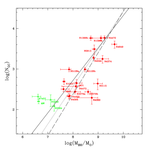
Figure 1.— The log of the number of GCs versus the log of the SMBH mass for the 20 giant galaxies included in the final sample and listed in Table Exploring the Correlations between Globular Cluster Populations and Supermassive Black Holes in Giant Galaxies. The red filled circles mark galaxies with classical bulges and the green open triangles denote galaxies that may have pseudobulges, according to the literature. NGC 1399, NGC 3379, and NGC 5128 each have two values of SMBH mass that are given half-weight in the fitting process (see Table Exploring the Correlations between Globular Cluster Populations and Supermassive Black Holes in Giant Galaxies for more information). The solid line is the best-fit line for the 18 E/S0 galaxies in the sample (Equation 8). The dotted line is the best-fit line to the E/S0 galaxies from BT10 and the dashed line is the best-fit relation for E galaxies from HH11.

So that I can compare my results directly to those of the previous studies on this topic, I have used the same statistical analysis methods employed by BT10 and HH11. Specifically, I have fitted lines to the data included in Figure 1 using the $\chi^{2}$-minimization method described in Tremaine et al. (2002) and Press et al. (1992). The method, called fitexy in Press et al. (1992), computes a best-fit linear relation of the form:

$${\rm y=\alpha+\beta x},$$ (3)

while taking into account the errors in both $x$ and $y$. The quantity

$$\rm{\chi^{2}=\sum_{i=1}^{N}\frac{{(y_{i}-\alpha-\beta x_{i})}^{2}}{\epsilon_{yi}^{2}+\beta^{2}\epsilon_{xi}^{2}}}$$ (4)

is minimized in the fitting process; here, $\epsilon_{xi}$ and $\epsilon_{yi}$ are the errors on $x$ and $y$, respectively. The errors are assumed to be symmetric, so I have calculated error bars on logarithmic quantities by averaging the high and low error bars; i.e., the error on each quantity is:

$$\rm{{\sigma_{log~{}i}={1/2}[log(i+\sigma_{i})-log(i-\sigma_{i})]}},$$ (5)

where $i$ in this case is either $N_{\rm GC}$ or $M_{\rm SMBH}$.

BT10 included thirteen elliptical and S0 galaxies in their $N_{\rm GC}$-$M_{\rm SMBH}$ fit; their best-fit relation is plotted as a dotted line in Figure 1 and is given in their paper in the form:

$$\rm{{log\frac{M_{\rm SMBH}}{M_{\odot}}=(8.14\pm 0.04)+(1.08\pm 0.04)log\frac{N_{GC}}{500}}}$$ (6)

HH11 fitted the $N_{\rm GC}$-$M_{\rm SMBH}$ correlation using 18 ellipticals from their sample of 33 galaxies and termed this their “baseline relation”. It is plotted as a dashed line in Figure 1 and can be written (following the format of the best-fit line from BT10) as:

$$\rm{{log\frac{M_{\rm SMBH}}{M_{\odot}}=(8.30\pm 0.29)+(0.98\pm 0.10)log\frac{N_{GC}}{500}}}$$ (7)

The galaxies with log($M_{\rm SMBH}$/$M_{\odot}$) greater than $\sim$7.5 in Figure 1 generally do seem to follow the linear relations of BT10 and HH11, but with a few galaxies (NGC 4649, NGC 3115, and NGC 4350) deviating from the lines. The group of four galaxies with the lowest SMBH masses (NGC 7457, NGC7332, the Milky Way, and NGC3384) also lie somewhat off the BT10 and HH11 relations. If I follow BT10 and include all 18 E/S0 galaxies in my fit, I derive the following best-fit relation:

$$\rm{{log\frac{M_{\rm SMBH}}{M_{\odot}}=(8.04\pm 0.03)+(1.22\pm 0.06)log\frac{N_{GC}}{500}}}$$ (8)

This relationship is plotted as a solid line in Figure 1. It has a steeper slope than the relations from both BT10 and HH11, although the slope and intercept differ from the previous values by less than 3$\sigma$, so are nevertheless consistent within the errors.

To assess the quality of the fits in their paper, BT10 calculated the $\chi^{2}$ per degree of freedom, which is often called the “reduced $\chi^{2}$”. Normally when one fits a line, the number of degrees of freedom is $N-2$, where $N$ is the number of data points included in the fit. BT10 used $N-4$ to normalize their $\chi^{2}$ values because three of the points they used are related (the three galaxies that each have two SMBH mass determinations in Table Exploring the Correlations between Globular Cluster Populations and Supermassive Black Holes in Giant Galaxies) and the inclusion of these points likely reduces the true number of degrees of freedom (Tremaine 2011, private communication). For their sample of 13 E/S0 galaxies, BT10’s best-fit $N_{\rm GC}$-$M_{\rm SMBH}$ line yields a reduced $\chi^{2}$ $=$ $\chi^{2}/(N-4)$ $=$ 6.6. For my sample of 18 E/S0 galaxies (including the same three galaxies with multiple SMBH measurements) my best-fit relation yields $\chi^{2}/(N-4)$ $=$ 10.4 and $\chi^{2}/(N-2)$ $=$ 9.3. Therefore, although I have limited my sample to galaxies with relatively well-determined $N_{\rm GC}$ values, the result is a $N_{\rm GC}$-$M_{\rm SMBH}$ fit of lower quality (as measured by the reduced $\chi^{2}$) than the fit produced by BT10 for their galaxy sample. On the other hand, the errors on my best-fit slope and intercept in Equation 8 are smaller than the errors on those quantities in the HH11 fit and comparable to the errors in the BT10 fit.

One way that previous authors have used to gauge the strength or quality of the correlation, as well as to account for the possibility that there is an intrinsic dispersion in the $N_{\rm GC}$-$M_{\rm SMBH}$ relation, is to add an additional dispersion term to one of the measurement errors and repeat the fitting process (cf. Tremaine et al. 2002, BT10, Snyder et al. 2011). The assumptions here are that the measurement errors are accurate and that there is some underlying, real galaxy-to-galaxy scatter present in the galaxy properties. With this type of approach, the amount of additional scatter that produces a reduced $\chi^{2}$ $\sim$ 1 is inferred to be the true intrinsic dispersion of the quantity. To implement this, one replaces the quantity $\epsilon_{yi}^{2}$ in Equation 4 with $(\epsilon_{yi}^{2}+\epsilon_{0}^{2})^{1/2}$ and performs the fitting procedure, adjusting $\epsilon_{0}$ until the value of the reduced $\chi^{2}$ is 1. Smaller values of $\epsilon_{0}$ are then interpreted as indicating a tighter correlation between the two quantities in the fit.

For my sample of 18 E/S0 galaxies, adding an intrinsic scatter of $\epsilon_{0}$ $\sim$ 0.45 dex in quadrature to either log $N_{\rm GC}$ or log $M_{\rm SMBH}$ produces a fit with reduced $\chi^{2}$ $\sim$ 1. The slope and intercept of the resultant fit are (using the notation from Equation 3) $\beta$ $=$ 1.11$\pm$0.19 and $\alpha$ $=$ 8.10$\pm$0.11, which are the same within the errors as the slope and intercept derived with no additional intrinsic scatter (Equation 8). For completeness, I should note that another approach sometimes seen in the literature is to simply add an intrinsic scatter term directly to the measurement errors, i.e., $\epsilon_{yi}$ $=$ $\epsilon_{yi}$ $+$ $\epsilon_{0}$ and then perform the fitting process. In this case, $\epsilon_{0}$ $\sim$ 0.3 dex (which corresponds to a linear factor of $\sim$2) needs to be added to the errors in order to produce reduced $\chi^{2}$ of unity for the E/S0 galaxy sample.

When I include all the galaxies in the sample (20 ellipticals, S0s, and spiral galaxies) and calculate the best-fit relation between $N_{\rm GC}$ and $M_{\rm SMBH}$  the result is:

$$\rm{{log\frac{M_{\rm SMBH}}{M_{\odot}}=(7.91\pm 0.03)+(1.52\pm 0.06)log\frac{N_{GC}}{500}}}$$ (9)

Including the two spiral galaxies in the fit steepens the slope of the relation not because of the data point for M31, which lies very close to the best-fitting relation for the E/S0 galaxies, but because of the data point for the Milky Way, which has comparatively small error bars and deviates significantly from the best-fitting E/S0 relation. The quality of this fit (as measured by reduced $\chi^{2}$) is degraded compared to the fit that includes only E/S0 galaxies; here, $\chi^{2}$/$(N-4)$ $=$ 12.4 and $\chi^{2}$/$(N-2)$ $=$ 11.2. The scatter as measured by the $\epsilon_{0}$ parameter is also larger: one must add $\epsilon_{0}$ $=$ 0.50 in quadrature to the errors in order to produce a reduced $\chi^{2}$ value of $\sim$1. Note that the results (slopes, intercepts, $\chi^{2}$ values, etc.) of the $N_{\rm GC}$$-$$M_{\rm SMBH}$ fitting process described in this section and in later sections of the paper are summarized in Table 2. The table lists: the sample used in the fitting process, the number of points in the sample, the intercept and slope of the best-fitting relation, the reduced $\chi^{2}$ values, and the value of the intrinsic scatter ($\epsilon_{0}$).

3.2. $M$-$\sigma$ Relation for the Galaxy Sample

Another useful or relevant comparison comes from determining, for my galaxy sample, whether a tighter correlation exists for $N_{\rm GC}$-$M_{\rm SMBH}$ or for $M_{\rm SMBH}$-$\sigma$. BT10 found that the former produced a higher-quality fit and therefore a stronger correlation. Figure 2 shows the $M_{\rm SMBH}$-$\sigma$ relation for my 20-galaxy sample. As in Figure 1, three galaxies are plotted twice and given half-weight in the fits. Galaxies with classical bulges are again represented by red filled circles and galaxies with pseudobulges are plotted with green open triangles; see Section 3.4.2 for more discussion.

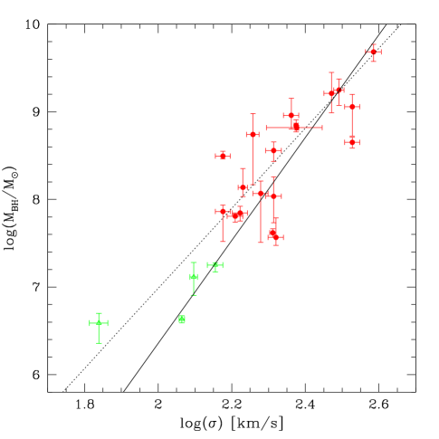
Figure 2.— The log of the SMBH mass versus the log of the velocity dispersion of the galaxy (for early-type galaxies) or the bulge (for spiral galaxies) for the 20 giant galaxies in Table Exploring the Correlations between Globular Cluster Populations and Supermassive Black Holes in Giant Galaxies. Red filled circles denote galaxies with classical bulges and green open triangles represent galaxies classified in the literature as having pseudobulges. Three galaxies are plotted twice and given half-weight in the fitting process (see Table Exploring the Correlations between Globular Cluster Populations and Supermassive Black Holes in Giant Galaxies). The solid line is the best-fitting line for all 20 galaxies (Equation 10) and the dotted line is the best-fit $M$-$\sigma$ relation from BT10.

I used the fitexy method to fit a line to the 20 galaxies in Figure 2. The result is shown as a solid line in the figure and can be written:

$${\rm{log\frac{M_{\rm SMBH}}{M_{\odot}}=(8.12\pm 0.03)+(5.87\pm 0.20)log\frac{\sigma}{200~{}km~{}s^{-1}}}}$$ (10)

The fit yields reduced $\chi^{2}$ values of $\chi^{2}/(N-4)$ $=$ 13.0 and $\chi^{2}/(N-2)$ $=$ 11.8. When I limit the galaxy sample to only the 18 E/S0 galaxies (i.e., excluding the Milky Way and M31), the best-fit line becomes:

$${\rm{log\frac{M_{\rm SMBH}}{M_{\odot}}=(8.15\pm 0.03)+(5.34\pm 0.27)log\frac{\sigma}{200~{}km~{}s^{-1}}}}$$ (11)

Both the error on the intercept and the reduced $\chi^{2}$ values become slightly larger in this case; here, $\chi^{2}/(N-4)$ $=$ 13.8 and $\chi^{2}/(N-2)$ $=$ 12.4. For both the full galaxy sample and the E/S0 sample, adding an additional scatter of $\epsilon_{0}$ $\sim$ 0.4 dex in quadrature to the errors on the log of the SMBH masses brings the reduced $\chi^{2}$ values to $\sim$1.

The corresponding best-fit $M$-$\sigma$ relation found by BT10 for their sample of 13 E/S0 galaxies is plotted as a dotted line in Figure 2 and is:

$${\rm{log\frac{M_{\rm SMBH}}{M_{\odot}}=(8.36\pm 0.04)+(4.57\pm 0.25)log\frac{\sigma}{200~{}km~{}s^{-1}}}}$$ (12)

BT10 found that both the reduced $\chi^{2}$ value and the amount of scatter in their best-fitting $N_{\rm GC}$-$M_{\rm SMBH}$ relation were smaller than those of their best-fitting $M$-$\sigma$ relation; thus, they found that $N_{\rm GC}$ is a better predictor of SMBH mass than is velocity dispersion $\sigma$. I find mixed results when I compare the quality of the $N_{\rm GC}$-$M_{\rm SMBH}$ and $M$-$\sigma$ correlations for my galaxy sample. As in BT10, the reduced $\chi^{2}$ values of my initial fits are slightly smaller for the $N_{\rm GC}$-$M_{\rm SMBH}$ correlation than for the $M$-$\sigma$ relation. The errors on the coefficients of my best-fit lines are likewise smaller for the $N_{\rm GC}$-$M_{\rm SMBH}$ relation than for the $M$-$\sigma$ relation. However, roughly the same amount of scatter ($\epsilon_{0}$ $\sim$ 0.4 dex) needs to be added in quadrature to the errors on the data points in both the $N_{\rm GC}$-$M_{\rm SMBH}$ and $M$-$\sigma$ fits in order to bring the reduced $\chi^{2}$ values to unity.

Finally I should note for the sake of completeness that the slope of the SMBH mass $-$ velocity dispersion relation derived for my sample of E/S0 galaxies (5.34$\pm$0.27) is consistent within $<$3 times the errors with the corresponding relation from BT10, as well as with the derived slopes from other recent giant galaxy studies. For example, Ferrarese & Ford (2005) find the slope of the $M$-$\sigma$ relation to be 4.86$\pm$0.43, Tremaine et al. (2002) derive 4.02$\pm$0.32, and Gultekin et al. (2009) calculate a slope of 3.96$\pm$0.42 for ellipticals and 4.24$\pm$0.41 for both early- and late-types. This is not surprising, of course, since the SMBH mass and velocity data I used were largely drawn from the same published measurements used by these authors (although I have rescaled the SMBH masses to the distances assumed for the GC system studies).

3.3. Are Metal-Poor or Metal-Rich GCs Better at Tracing SMBH Mass?

As I mentioned briefly in Section 2.2.1, the broadband colors of GCs can be an indicator of their metallicities. It is generally true that for old (${}_{>}\atop{{}^{\sim}}$2$-$3 Gyr) stellar populations, optical colors primarily trace metallicity, with blue colors corresponding to metal-poor populations and red to metal-rich. This is caused by a combination of factors, such as line blanketing due to the presence of metals in stellar atmospheres and metal-rich stars having lower equilibrium temperatures on the main sequence and in later evolutionary stages (e.g., Schwarzschild et al. 1955, Sweigart & Gross 1978). The GC systems of many giant galaxies have color distributions with more than one peak (e.g., Zepf & Ashman 1993, Kundu & Whitmore 2001, Peng et al. 2006), so these multiple peaks seem to imply the presence of GC populations with different metallicities, presumably formed in different episodes. Spectroscopic metallicities, kinematic studies, and near-IR colors of GCs confirm this interpretation (e.g., Kundu & Zepf 2007, Strader et al. 2007, Beasley et al. 2008, Alves-Brito et al. 2011). The fact that the Milky Way and M31 also have two populations of GCs with different metallicities and kinematics (Zinn 1985, Perrett et al. 2002) seems to suggest that multiple GC populations may be a common characteristic of giant galaxies.

The overarching goal of many of the studies of extragalactic GC systems in recent years has been to understand the range of giant galaxy GC system properties — including the presence of multiple peaks in GC color/metallicity distributions — within the larger context of galaxy formation and evolution (see the review on this subject by Brodie & Strader 2006). Over time a general picture has developed that incorporates aspects of a number of different scenarios for GC and galaxy formation (e.g., Ashman & Zepf 1992, Forbes et al. 1997, Cote et al. 1998, Beasley et al. 2002, Santos 2003, Rhode, Zepf, & Santos 2005, Muratov & Gnedin 2010). The precise details are not yet well-established, but the data seem to point toward a picture (that Brodie & Strader 2006 term the“synthesis scenario”) in which metal-poor GCs were formed when low-mass, gas-rich protogalactic fragments collided and merged at high redshift ($z$$\sim$10$-$15) and metal-rich GCs were formed during dissipational mergers at later times. In this picture the blue, metal-poor GC populations in giant galaxies are therefore fossils left over from the first epoch of GC and galaxy assembly. The effect of cosmological “biasing” may also be an important piece of the puzzle; massive galaxy halos located in dense environments are expected to have a larger proportion of their mass accumulated by a given redshift than lower-mass galaxies in lower-density environments (e.g., Sheth 2003).

In some models, this initial phase of GC formation is truncated or suppressed by some mechanism around $z$$\sim$10 for a brief period of time. Santos (2003) suggests reionization would serve as such a truncation mechanism, and would suppress both GC and structure formation for ${}_{<}\atop{{}^{\sim}}$1 Gyr. Forbes et al. (1997) suggest that some more localized form of feedback from the first generation of stars and GCs could shut off metal-poor GC formation for a few Gyr. In the semi-analytic simulations of Muratov & Gnedin (2010), blue, metal-poor GCs are formed in early mergers of low-mass protogalactic clumps, whereas both blue and red GCs are formed in later mergers of more massive galaxies. In any case, after the initial epoch of galaxy assembly and GC formation, more GCs are expected to form each time the host galaxy undergoes a gas-rich, dissipational major merger. Because stellar evolution enriches the interstellar and intergalactic medium over time, any new GCs that are created in subsequent events are expected to be more metal-rich than the earliest generation. This type of broad outline can explain the metallicity gap between GC subpopulations of similar age, as well as several other observations, such as: more massive galaxies have larger relative numbers of blue, metal-poor GCs (Rhode et al. 2005, 2007); the average metallicity of metal-poor GCs in more luminous galaxies is slightly higher than that in less luminous galaxies (Strader, Brodie, & Forbes 2004); and blue, metal-poor GCs have different spatial distributions than red, metal-rich GCs in some galaxies (e.g., Zinn 1985, Moore et al. 2006, Dirsch et al. 2003, Bassino et al. 2006). On the other hand, this rough outline ignores complicating effects such as dynamical destruction of GCs over time, which may vary depending on the properties of the GC itself and/or its parent galaxy (e.g., Vesperini 2000). It also ignores the possibility that galaxy mergers may themselves destroy a significant fraction of the GCs present in the progenitor merging galaxies, not just create new ones (Kruijssen et al. 2012). Both of these effects may have substantially modified the trends in GC numbers in different galaxies that we measure today (at $z$$=$0) and may make it considerably more difficult to accurately interpret our observations.

A scenario like this may also have implications for the observed correlation between $N_{\rm GC}$ and $M_{\rm SMBH}$. BT10 briefly speculate that the apparent connection between $N_{\rm GC}$ and $M_{\rm SMBH}$ may arise because both SMBHs and GC populations grow via recent major galaxy mergers. Alternatively, SMBHs and GCs may be linked because they originate at high-$z$ in gas-rich young galaxies. We can consider these two possibilities in the context of the broad picture I have outlined of the formation of metal-poor and metal-rich GC subpopulations. If SMBHs are primordial objects and their properties are set during the initial formation epoch of their host galaxies, one might expect a strong correlation between the numbers of blue, metal-poor GCs in the galaxy and the SMBH mass. If, on the other hand, SMBHs are fed primarily by recent major galaxy mergers, then one might expect a stronger correlation between $M_{\rm SMBH}$ and the numbers of red, metal-rich GCs in a galaxy, since the metal-rich GC population is likely built up over time during major merger events.

BT10 examined the $N_{\rm GC}$$-$$M_{\rm SMBH}$ relation separately for blue and red GCs in their sample of 13 galaxies but found that the correlations were similar in quality; as they note, the fractions of blue and red GCs in giant galaxies appear to be fairly constant. The blue fraction $f_{\rm blue}$ for my sample of 20 galaxies is listed in column 11 of Table Exploring the Correlations between Globular Cluster Populations and Supermassive Black Holes in Giant Galaxies. The blue GC fractions for the galaxies range from 0.52 to 0.72 and the mean $f_{\rm blue}$ is 0.61, with a standard deviation of 0.07. Figure 3 shows the log of the number of blue GCs and red GCs versus the log of the SMBH mass plotted in the top panel and bottom panel, respectively. (Galaxies with classical bulges and pseudobulges are again shown with different symbols.) The plots look similar and there are only small differences in the fitting results from fitexy. Counting only the blue GCs, the best-fit relation for the 18 E/S0 galaxies in my sample becomes:

$$\rm{{log\frac{M_{\rm SMBH}}{M_{\odot}}=(8.32\pm 0.03)+(1.23\pm 0.06)log\frac{N_{GC,blue}}{500}}}$$ (13)

Including only the red GCs in my E/S0 galaxies yields:

$$\rm{{log\frac{M_{\rm SMBH}}{M_{\odot}}=(8.52\pm 0.03)+(1.20\pm 0.05)log\frac{N_{GC,red}}{500}}}$$ (14)

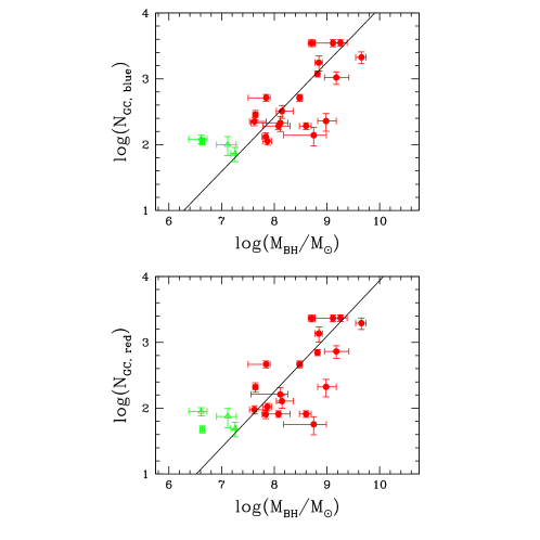
Figure 3.— The log of $N_{\rm GC}$ versus the log of $M_{\rm SMBH}$ for the blue, metal-poor GCs (top) and red, metal-rich GCs (bottom) for the sample of 20 giant galaxies in this study. Galaxies with classical bulges and pseudobulges are marked as in the other figures. NGC 1399, NGC 3379, and NGC 5128 each have two values of SMBH mass that are given half-weight in the fitting process. The solid lines are the best-fit lines derived using the 18 E/S0 galaxies in the sample (Equations 13 and 14).

These relations are shown as solid lines in the appropriate plot (blue GCs in the top panel, red GCs in the bottom panel) in Figure 3. The blue-only GC sample yields a slightly smaller reduced $\chi^{2}$ value than the red GC sample; the former yields $\chi^{2}$/(N-4) $=$ 10.6 for the blue GCs vs. $\chi^{2}$/(N-4) $=$ 11.0 for the red GCs. The blue GC sample also needs slightly less additional scatter added to the data points than the red GC sample in order to produce a reduced $\chi^{2}$ $\sim$ 1; the blue GCs require $\epsilon_{0}$ $=$ 0.48 dex vs. $\epsilon_{0}$ $=$ 0.51 dex for the red GCs. Note that the blue GC fractions that appear in Table Exploring the Correlations between Globular Cluster Populations and Supermassive Black Holes in Giant Galaxies do not have accompanying uncertainties listed. Assigning an accurate error to the blue fraction can be difficult, especially when data are being compiled from different studies that use a variety of methods for determining blue and red GC fractions (e.g., fitting with mixture modeling code, or simply dividing a completeness-corrected sample at a certain fiducial color) and in many cases no error is given on the estimated blue or red fraction. To investigate how possible uncertainties on the blue and red fraction would contribute to the relation between number of blue or red GCs and SMBH mass, I incorporated a 10% error on the blue and red fractions into the total errors on $N_{\rm GC,blue}$ and $N_{\rm GC,red}$ and ran fitexy again for the 18 E/S0 galaxies. Including only the blue GCs, and incorporating a 10% error on the blue fractions given in Table Exploring the Correlations between Globular Cluster Populations and Supermassive Black Holes in Giant Galaxies, the best-fit relation for the 18 E/S0 galaxies is:

$$\rm{{log\frac{M_{\rm SMBH}}{M_{\odot}}=(8.32\pm 0.03)+(1.29\pm 0.07)log\frac{N_{GC,blue}}{500}}}$$ (15)

Including only the red GCs and including a 10% error on the red fraction yields for the E/S0 galaxies:

$$\rm{{log\frac{M_{\rm SMBH}}{M_{\odot}}=(8.52\pm 0.04)+(1.23\pm 0.06)log\frac{N_{GC,red}}{500}}}$$ (16)

With these additional error estimates included, the reduced $\chi^{2}$ for the fit to the blue GC sample is $\chi^{2}$/(N-4) $=$ 9.0 and the fit to the red GC sample yields $\chi^{2}$/(N-4) $=$ 9.5.

If the blue GC population were a better tracer of SMBH mass than the red GC population and if the overall picture of hierarchical galaxy and GC formation actually holds true, it might suggest that the masses of the SMBHs are set during the initial formation epoch of the host galaxies and are less dependent on subsequent mergers that occur. However, given that reduced $\chi^{2}$ values are themselves subject to uncertainty (on the order of a few tenths in this case; e.g., Andrae et al. 2010), the very small difference in reduced $\chi^{2}$ between the blue and red GC populations is not significant.

3.4. Trends with Host Galaxy Morphology

3.4.1 Splitting the Sample by Hubble Type

HH11 compiled a larger sample of galaxies than BT10 with a wider range of morphological types and hence were able to investigate how the correlation of $N_{\rm GC}$ with $M_{\rm SMBH}$ varies with galaxy morphology. The HH11 sample included 21 elliptical galaxies, eight S0 galaxies, and four spiral galaxies. My more restricted sample of 20 galaxies with reliable GC system properties includes 10 ellipticals, eight lenticular galaxies, and two spiral galaxies, so I can also explore this issue, although to a more limited extent than HH11. Figure 4 shows log $N_{\rm GC}$ versus log $M_{\rm SMBH}$ for the 20 galaxies separated by morphological type, with ellipticals, S0 galaxies, and spiral galaxies plotted from left to right. The best-fit $N_{\rm GC}$$-$$M_{\rm SMBH}$ relation for E/S0s (Equation 8) is shown as a fiducial; it appears in all three plots as a solid line. The three galaxies with two $M_{\rm SMBH}$ values, NGC 1399, NGC 3379, and NGC 5128 are (as before) plotted twice; all three are Es and thus are included in the leftmost plot. The morphological type of NGC 4594 (M104, a.k.a. the Sombrero galaxy) is listed in Table Exploring the Correlations between Globular Cluster Populations and Supermassive Black Holes in Giant Galaxies as “S0/Sa” and I have included this galaxy in the S0 plot; it is the point with the largest $N_{\rm GC}$ value, lying very close to the E/S0 best-fit line. NGC 4594 is often classified by appearance as an Sa spiral galaxy, probably at least in part because its nearly edge-on orientation makes its dust lane and disk appear more prominent. Its quantitative properties, however, are more like that of an S0 galaxy: its bulge-to-disk ratio is $\sim$6, bulge fraction ($B/T$) is 0.86 (Kent 1988), and its $B-V$ color is 0.84 (RC3; de Vaucouleurs et al. 1991). In any case, it is unclear whether NGC 4594 belongs in the S0 plot (middle) or the spiral galaxy plot (right) in Figure 4.

Figure 4.— The same data as in Figure 1, except with the 20 galaxies in the final sample separated by morphological type. Red filled circles again represent galaxies with classical bulges and green open triangles show galaxies with pseudobulges. The solid line is the best-fit $N_{\rm GC}$$-$$M_{\rm SMBH}$ relation for E/S0 galaxies (Equation 8). NGC 4594 is included in the S0 plot, although this galaxy is sometimes classified as an Sa. The dotted line in the middle panel is the best-fitting relation for the S0s with NGC 4594 included, and the dashed line is the best-fitting relation with NGC 4594 excluded.

HH11 found that the elliptical galaxies in their sample exhibited a strong correlation between $N_{\rm GC}$ and $M_{\rm SMBH}$ and that the spiral galaxies, with the exception of the Milky Way, closely followed the same relation. The S0 galaxies in their sample, on the other hand, showed “no clear trend” in a log($N_{\rm GC}$) versus log ($M_{\rm SMBH}$) plot. The results for my sample of 20 galaxies are similar to those of HH11. The 10 elliptical galaxies in the left panel of Figure 4 closely follow the fiducial E/S0 line. When I fit the $N_{\rm GC}$$-$$M_{\rm SMBH}$ relation for just these 10 elliptical galaxies, the result is

$$\rm{{log\frac{M_{\rm SMBH}}{M_{\odot}}=(8.17\pm 0.04)+(0.95\pm 0.07)log\frac{N_{GC}}{500}}}$$ (17)

with a reduced $\chi^{2}$ values of $\chi^{2}$/(N$-$4) $=$ 9.4 and $\chi^{2}$/(N$-$2) $=$ 7.7 and $\epsilon_{0}$ $=$ 0.37. (For comparison, the slope and intercept of the elliptical-only relation from HH11 are 0.98$\pm$0.10 and 8.30$\pm$0.29, respectively; see Equation 7.) The slope and intercept of this line are the same within the errors as those for my E/S0 sample (Equation 8). The spiral galaxy points in the rightmost panel in the figure both fall close to the E/S0 line. In the middle panel of S0 galaxies, NGC 4594 (which may be an Sa or an S0 galaxy) also falls close to the E/S0 best-fit line. The other S0 galaxies have a relatively small range of $N_{\rm GC}$ values ($\sim$120$-$500) but a large range in SMBH mass. Fitting a line to the S0 points with NGC 4594 included changes the slope of the best-fit $N_{\rm GC}$$-$$M_{\rm SMBH}$ relation to 1.6$\pm$0.1. Excluding NGC 4594 and fitting the points for the remaining S0 galaxies yields only a very shallow trend of slightly increasing log($N_{\rm GC}$) with increasing log($M_{\rm SMBH}$) with a slope of 10.2$\pm$5.5; this is not consistent with the best-fitting relations for the E/S0 sample or the elliptical-only sample.

3.4.2 Classical Bulges vs. Pseudobulges

Before drawing any conclusions about trends in morphology, it is worth exploring one more morphology-related issue and asking whether the behavior of galaxies with classical bulges differs from that of galaxies with pseudobulges in the $N_{\rm GC}$$-$$M_{\rm SMBH}$ plane. Classical bulges are thought to form via relatively rapid (i.e., evolution on dynamical time scales), violent processes like dissipational collapse and mergers. In contrast, pseudobulges appear to be built up gradually over a few billion years by “secular”, internal processes in galaxy disks, like gas transport aided by bar instabilities and spiral structure (Kormendy & Kennicutt, 2004). By this definition, elliptical galaxies are in the “classical” bulge category and S0 and spiral galaxies can fall in either category, although Kormendy & Kennicutt (2004) note that the type of secular evolution that produces pseudobulges is most likely to be important in intermediate- to late-type galaxies (Sbc galaxies and later). Kormendy, Bender, & Cornell (2011) recently analyzed a sample of $\sim$50 spiral, S0, and elliptical galaxies and found that the disk galaxies with pseudobulges do not follow the same $M$-$\sigma$ relation as ellipticals and classical-bulge galaxies. Galaxies in their sample with pseudobulges at least showed a much larger scatter in the $M$-$\sigma$ plane and arguably displayed no correlation at all.

To examine whether the $N_{\rm GC}$$-$$M_{\rm SMBH}$ correlation changes for galaxies with pseudobulges vs. those with classical bulges, I searched the literature to find bulge classifications for the 20 galaxies in my sample. The elliptical galaxies all fall in the “classical” category. I found classifications for the S0 and spiral galaxies primarily in the lists included in Kormendy & Kennicutt (2004), Fisher & Drory (2008, 2010), and Kormendy et al. (2011). Based on my literature search, four of the 20 galaxies in my sample may have pseudobulges: the Milky Way (Shen et al. 2010 and references therein), NGC 3384 (Kormendy et al. 2011, Pinkney et al. 2003), NGC 7332 (Pinkney et al. 2003, Falcon-Barroso et al. 2004), and NGC 7457 (Kormendy 1993, Kormendy & Kennicutt 2004). Classifying a galaxy as possessing a pseudobulge is notoriously difficult (Kormendy & Kennicutt 2004), so none of these four galaxies has been unequivocally shown to have a pseudobulge rather than a classical bulge. The classifications of NGC 7332 and NGC 7457 are especially uncertain. The evidence that NGC 7332 has a pseudobulge is merely circumstantial: observations with an integral-field unit show that this galaxy has a bar and a cold, counter-rotating stellar disk, as well as stellar kinematics in its inner regions that are typical of a “boxy bulge” (Falcon-Barroso et al. 2004). Together these imply a pseudobulge rather than a classical bulge. In the case of NGC 7457, Kormendy (1993) found that its central velocity dispersion is very small for its bulge luminosity (i.e., its bulge lies well below the Faber-Jackson relation; Faber & Jackson 1976); this is one of the properties Kormendy & Kennicutt (2004) identify with pseudobulges. Pinkney et al. (2003) confirmed that NGC 7457 has central stellar kinematics characteristic of a pseudobulge, but Kormendy et al. (2011) place this galaxy in the “classical bulge” category in their paper.

The four galaxies that may have pseudobulges are designated in Figures 1$-$4 with green open triangles, while the classical-bulge and elliptical galaxies are plotted with red filled circles. Figure 1 shows the full sample of 20 galaxies in the $N_{\rm GC}$$-$$M_{\rm SMBH}$ plane; the four pseudobulge galaxies are in the lower left of the diagram. In Figure 4 the galaxies are split up by morphology, so three of the pseudobulge galaxies (NGC 3384, NGC 7332, and NGC 7457) appear in the middle panel and the fourth (the Milky Way) appears on the spiral galaxy panel on the right. Three of the four pseudobulge galaxies are systematically above and to the left of the best-fit E/S0 relation in the $N_{\rm GC}$$-$$M_{\rm SMBH}$ plane, i.e., their GC populations are too large for their SMBH masses (or their SMBH masses are too small for their GC numbers). The other pseudobulge galaxy (NGC 3384) lies on the relation. On the other hand, there are so few pseudobulge points and there is so much scatter around the best-fitting $N_{\rm GC}$$-$$M_{\rm SMBH}$ relation that it is not possible to determine from this sample whether the pseudobulge galaxies are truly outliers or are simply, by coincidence, scattering in the same direction.

Lastly, I should note that the galaxies with pseudobulges seem to fall along the same $M$-$\sigma$ relation (Figure 2) as the rest of the galaxies in the full sample. Two of the four galaxies with pseudobulges (NGC 3384 and NGC 7332) intersect the best-fitting line for the full sample (the solid line in Figure 2), and a third galaxy (the Milky Way) lies very close to the line. Only NGC 7457 scatters far away from the best-fit relation (and its classification as a pseudobulge galaxy was uncertain). As mentioned earlier, Kormendy et al. (2011) concluded that pseudobulge galaxies do not follow the $M$-$\sigma$ relation for ellipticals and classical-bulge galaxies. The galaxies that seemed to deviate from their best-fitting $M$-$\sigma$ relation in Kormendy et al. were located in a specific region of the $M$-$\sigma$ plane: below SMBH masses log(M/$M_{\odot}$) ${}_{<}\atop{{}^{\sim}}$8 and velocity dispersions log($\sigma$) ${}_{<}\atop{{}^{\sim}}$2.2. Kormendy et al. (2011) had $\sim$15 galaxies with pseudobulges in that area of the plane. My sample has very few objects in that region of the $M$-$\sigma$ plane so it is difficult to assess whether the data presented here contradict their conclusions or not.

3.4.3 What Might the Trends in Morphology Mean?

In part because of the small numbers of S0, spiral, and pseudobulge galaxies in the sample, it is not clear what the pseudobulge vs. classical bulge values in the $N_{\rm GC}$$-$$M_{\rm SMBH}$ plane and the data in Figure 4 are indicating. It is possible that there is: (1) a marked trend of increasing $N_{\rm GC}$ with increasing  $M_{\rm SMBH}$ mass for elliptical galaxies and perhaps spiral galaxies, but a much weaker trend for S0s; or (2) a clear trend in increasing $N_{\rm GC}$ with $M_{\rm SMBH}$ for classical-bulge galaxies but not for pseudobulge galaxies; or (3) an overall trend in $N_{\rm GC}$ vs. $M_{\rm SMBH}$ for giant galaxies, but with plenty of scatter, especially at lower $N_{\rm GC}$ and lower SMBH masses.

The situation implied by the first possibility does not have an obvious physical explanation; it is not clear what mechanism would cause S0 galaxies to have a limited range of $N_{\rm GC}$ values but a wide range of SMBH masses (log($M_{\rm SMBH}$/M_⊙) $\sim$ 6$-$9) while ellipticals have $N_{\rm GC}$ and $M_{\rm SMBH}$ values that are closely linked. Whatever direct or indirect correlation might be present between GC populations and SMBH masses in elliptical galaxies may, for some unknown reason, break down for most S0 galaxies.

The second possibility, on the other hand, could make sense in terms of how we think both SMBHs and bulges grow. Kormendy et al. (2011) succinctly describe two different “modes” for the feeding and growth of SMBHs, that echo the two different growth modes for building galaxy bulges. One mode is violent, rapid mergers that drive gas infall and efficiently build up both classical bulges and the seed SMBHs within them. The other mode is the more gradual, local, stochastic growth (e.g., build-up of a central concentration in a disk galaxy via disk instabilities and gas-flow along bars) that builds pseudobulges, and that may also result in slower and more modest growth of SMBHs. If GC populations, classical bulges, and SMBHs can all be grown and significantly increased via mergers, one might imagine that galaxies with classical bulges are then also likely to have $N_{\rm GC}$ values and $M_{\rm SMBH}$ values that increase together. Galaxies with more quiescent histories, that perhaps made GCs in their early assembly stages at high-$z$ but did not do much more to supplement their GC populations over time, perhaps would end up today as disk galaxies with a pseudobulge, a modest-sized SMBH, and a weaker correlation between their $M_{\rm SMBH}$ and $N_{\rm GC}$ values. In other words, whatever correlation between $N_{\rm GC}$ and $M_{\rm SMBH}$ was set up in the earliest stages of a galaxy’s assembly may be strengthened in galaxies that continue to grow via major mergers, but weakened in galaxies with pseudobulges that evolve more quiescently.

Finally, the third scenario mentioned above is that the $N_{\rm GC}$$-$$M_{\rm SMBH}$ correlation is generally present in giant galaxies but is weaker and has more scatter at lower $N_{\rm GC}$ values and lower SMBH masses, and by implication, lower-mass galaxies, since both $N_{\rm GC}$ and $M_{\rm SMBH}$ correlate with galaxy mass (see next section). If this is the case, the explanation could be similar to the scenario for possibility (2). Perhaps a common mechanism like major galaxy mergers drives the formation of very massive SMBHs and very populous GC systems in massive galaxies and this mechanism becomes less important in the evolution of lower-mass galaxies, their GC populations, and their SMBHs. The net effect would be that the GC numbers and SMBHs “decouple” (because the phenomenon that linked them in the first place, major gas-rich mergers, is no longer of primary importance in their evolution) and the correlation gets weaker with decreasing galaxy mass.

3.5. Correlations of $N_{\rm GC}$ with Other Galaxy Properties

3.5.1 Number of GCs Versus Galaxy Stellar Luminosity and Mass

The number of GCs in some giant galaxies has been observed to follow a rough correlation with galaxy luminosity, with $N_{\rm GC}$ $\propto$ $L^{\alpha}$, where $\alpha$ is between 1 and 2 (Ashman & Zepf 1998 and references therein). A sensible next step is to use the current galaxy sample to examine this and other correlations that $N_{\rm GC}$ has with galaxy properties, as well as to compare the strength of this correlation to the $N_{\rm GC}$$-$$M_{\rm SMBH}$ relation. To do this, I have supplemented the galaxies in the N$=$20 sample that I used in earlier sections of the paper with ten more galaxies with measured $N_{\rm GC}$ from my wide-field GC system survey. These ten additional galaxies have well-determined GC system properties (i.e., the criteria in Section 2.2.1 are met), but the galaxies were not included in the previous analysis because they do not have measured SMBH masses. The properties of these additional ten galaxies are listed in Table Exploring the Correlations between Globular Cluster Populations and Supermassive Black Holes in Giant Galaxies. The columns in the table are: galaxy name and morphological type; predicted SMBH mass calculated from the best-fitting $N_{\rm GC}$$-$$M_{\rm SMBH}$ relation (Equation 9; see Section 3.6 for details); central velocity dispersion; $M_{V}$ for the galaxy; distance to the galaxy in Mpc; number of GCs; GC specific frequencies $S_{N}$ and $T$; fraction of blue GCs in the GC system; and the reference for the GC system properties.

The left-hand side of Figure 5 shows the log of $N_{\rm GC}$ versus the log of the $V$-band luminosity in solar units, $L_{V}$/$L_{\odot}$, for the 30 galaxies listed in Tables Exploring the Correlations between Globular Cluster Populations and Supermassive Black Holes in Giant Galaxies and Exploring the Correlations between Globular Cluster Populations and Supermassive Black Holes in Giant Galaxies. The right-hand side of the same figure shows log of $N_{\rm GC}$ plotted against the log of the galaxy stellar mass in solar masses ($M_{*}$/$M_{\odot}$) for the same 30 galaxies. To calculate stellar masses for the galaxies, I combined their $M_{V}$ values with the Zepf & Ashman (1993) mass-to-light ratios discussed in Section 2.2.1. In both plots, galaxies from Table Exploring the Correlations between Globular Cluster Populations and Supermassive Black Holes in Giant Galaxies with classical bulges are designated with red filled circles and galaxies with pseudobulges with green open triangles, while the 10 additional galaxies from the wide-field survey are plotted with open stars. I searched the literature for bulge classifications for these additional 10 galaxies and found that one of the objects, the Sb spiral galaxy NGC 891, may have a pseudobulge; de Jong et al. (2008) characterize its bulge as a boxy pseudobulge based on surface photometry. The point representing NGC 891 is labeled in the plots. The point with the largest $N_{\rm GC}$ error bars in both plots is NGC 7331; this galaxy has a relatively low inclination ($i$$\sim$75 degrees) compared to the other spiral galaxies in the survey, which makes it difficult to detect GCs against the background of the galaxy’s spiral disk. The end result was a $N_{\rm GC}$ value that was relatively uncertain (Rhode et al. 2007). Lastly, note that there are only 30 points in the figure because the three galaxies that were plotted twice in the figures that included SMBH mass are only plotted once here (they each have only one value of $N_{\rm GC}$ and galaxy luminosity or stellar mass).

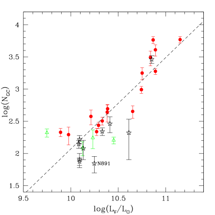
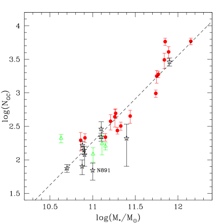
Figure 5.— The log of $N_{\rm GC}$ versus the log of the $V$-band luminosity and galaxy stellar mass for the 20 galaxies in Table Exploring the Correlations between Globular Cluster Populations and Supermassive Black Holes in Giant Galaxies and the ten galaxies from my wide-field survey in Table Exploring the Correlations between Globular Cluster Populations and Supermassive Black Holes in Giant Galaxies. Galaxies with classical bulges and pseudobulges in the Table Exploring the Correlations between Globular Cluster Populations and Supermassive Black Holes in Giant Galaxies sample are marked with red filled circles and green open triangles, respectively, as in the other figures. Galaxies from the wide-field survey are designated with open stars. The spiral galaxy NGC 891 (labeled on the plots) is not shown in green but may have a pseudobulge. The best-fit lines are plotted on the figures and given in Equations 18 and 19. The relation between $N_{\rm GC}$ and total galaxy luminosity yields $\chi^{2}/(N-2)$ $=$ 15.8 and the relation between $N_{\rm GC}$ and total galaxy stellar mass yields $\chi^{2}/(N-2)$ $=$ 8.9.

Fitting the 30 data points shown in the panels of Figure 5 yields the following best-fit linear relations:

$$\rm{{log\frac{L_{\rm V}}{L_{\odot}}=(10.44\pm 0.01)+(0.70\pm 0.02)log\frac{N_{GC}}{500}}}$$ (18)

and

$$\rm{{log\frac{M_{*}}{M_{\odot}}=(11.33\pm 0.01)+(0.78\pm 0.02)log\frac{N_{GC}}{500}}}$$ (19)

Written another way, these relationships mean $N_{\rm GC}$ $\propto$ $(L_{V}$/$L_{\odot})^{1.42}$ and $N_{\rm GC}$ $\propto$ $(M_{*}$/$M_{\odot})^{1.28}$, respectively. The reduced $\chi^{2}$ value for the fit between $N_{\rm GC}$ and total galaxy stellar mass is $\chi^{2}$/$(N-2)$ $=$ 8.9, compared to 15.8 for the $N_{\rm GC}$$-$luminosity fit. This makes sense given the appearance of the data: the log of the number of GCs shows a tight correlation with the log of the host galaxy stellar mass, whereas the log($N_{\rm GC}$) vs. log($L_{V}$) data show much more scatter, especially for the lower-luminosity galaxies with log($L_{V}$) $<$ 10.75. The intrinsic scatter is substantially smaller in this relation compared to any of the $N_{\rm GC}$$-$$M_{\rm SMBH}$ relations: adding $\epsilon_{0}$ $=$ 0.14 dex in quadrature to the errors brings the reduced $\chi^{2}$ value to $\sim$1. (For completeness, I also checked the fitting result for the 20-galaxy sample in Table Exploring the Correlations between Globular Cluster Populations and Supermassive Black Holes in Giant Galaxies, without the additional ten galaxies from the survey. For the N$=$20 sample, the intrinsic scatter remains small, at $\epsilon_{0}$ $=$ 0.15 dex.) The correlation between $N_{\rm GC}$ and galaxy stellar mass in Figure 5 is the strongest of any of the correlations analyzed in this paper. It is important to note that the reduced $\chi^{2}$ and $\epsilon_{0}$ values would be even smaller if errors on the galaxy luminosity or mass were included in the fits. Specifically, arbitrarily setting the galaxy mass error to 10% of the stellar mass yields a best-fitting line with the same slope and intercept (within the uncertainties on those coefficients) as the fit without errors on the mass, but with a $\chi^{2}$/$(N-2)$ $=$ 5.1. Setting the relative error on the galaxy stellar mass to 25% yields the same coefficients and $\chi^{2}$/$(N-2)$ $=$ 1.5. Even without error bars in the $x$-direction, the quality of the correlation between $N_{\rm GC}$ and galaxy mass is much better than the $N_{\rm GC}$$-$$M_{\rm SMBH}$ and $M$-$\sigma$ correlations explored in the earlier sections of the paper.

When I include only the blue, metal-poor or red, metal-rich GCs in $N_{\rm GC}$ and fit the data points versus total galaxy stellar mass, I find that the slope of the line remains the same within the errors, but that the quality of the fit is better for the blue GCs than for the red ones. The former yields $\chi^{2}$/$(N-2)$ $=$ 8.7 and $\epsilon_{0}$ $=$ 0.14 dex, whereas the latter yields $\chi^{2}$/$(N-2)$ $=$ 11.1 and $\epsilon_{0}$ $=$ 0.15 dex. The slightly improved fit yielded by the blue GCs may suggest that it is chiefly the blue, metal-poor GCs that are driving the correlation between $N_{\rm GC}$ and galaxy stellar mass.

One object in Figure 5, the S0 galaxy NGC 7457, has a particularly large value of $N_{\rm GC}$ for its stellar mass, and lies significantly off the best-fit relation. It is the lowest-mass galaxy in the sample, with log($M_{*}$/$M_{\odot}$) $=$ 10.6 but it has an estimated population of 210$\pm$30 GCs (Hargis et al. 2011). This galaxy is in a low-density environment ($\rho$ $=$ 0.13 Mpc^-3; Tully 1988) and its GC system was studied as part of our wide-field survey. There is not an obvious reason for its high $N_{\rm GC}$ value and high specific frequency ($S_{N}$ $=$ 3.1$\pm$0.7). Excluding NGC 7457 from the sample and fitting log($N_{\rm GC}$) vs. log($M_{*}$/$M_{\odot}$) yields the same coefficients as in Equation 19 within the errors and improves the fit, so that $\chi^{2}$/$(N-2)$ becomes 6.0 and $\epsilon_{0}$ becomes 0.10 dex.

Lastly, I should note that in addition to calculating total galaxy stellar masses from the $V$-band luminosity, I also computed stellar masses from $K$-band luminosity of each galaxy and used those to examine the relationship between $N_{\rm GC}$ and galaxy stellar mass. I combined the total $K$-band apparent magnitude listed in the NASA Extragalactic Database (NED) — which in turn come from either from the 2MASS Extended Source Catalog (Jarrett et al. 2000) or the 2MASS Large Galaxy Atlas (Jarrett et al. 2003) — with the adopted distance modulus to derive total $K$-band luminosity for each galaxy. I then applied the appropriate $K$-band mass-to-light ratio from Spitler et al. (2008) for each galaxy’s morphological type to calculate galaxy stellar mass. I fitted log($N_{\rm GC}$) vs. log($M_{*}$/$M_{\odot}$) for these $K$-band-derived masses and found that the best-fitting coefficients were similar to those in Equation 19 but the scatter in the plot was larger and the reduced $\chi^{2}$ values increased by a factor of $\sim$1.5. So at least for this specific data set, the $V$-band galaxy magnitudes and stellar masses produced better-quality results in terms of the correlation between number of GCs and galaxy stellar mass.

3.5.2 Number of GCs Versus Bulge Luminosity and Mass

The analysis in the previous section examined correlations of $N_{\rm GC}$ with the total stellar mass and luminosity of the host galaxy, but there are reasons why looking at $N_{\rm GC}$ versus the mass and luminosity of just the spheroidal component might make more sense. As mentioned in Section 1, the analysis of Snyder et al. (2011) indicated that the correlation between $N_{\rm GC}$ and $M_{\rm SMBH}$ arises because both of those quantities correlate with the binding energy or potential well depth of the bulge component of the host galaxy. It has been argued that at least some GCs are actually associated with galaxy bulges rather than with thick disks or halos. Specifically, the properties of the more metal-rich GC subpopulation of the Milky Way may indicate it is a bulge population (e.g., van den Bergh 1993). In this type of picture, the red, metal-rich GCs would then be an analogous population in other spiral and elliptical galaxies (e.g., Forbes, Brodie & Larsen 2001). In previous extragalactic GC system studies, the specific frequency $S_{N}$ is sometimes normalized using bulge luminosity rather than total luminosity for spiral galaxies. (e.g., Harris 1981, Cote et al. 2000, Forbes et al. 2001). For these reasons, I have also investigated the relationship between $N_{\rm GC}$ and galaxy luminosity and mass using the bulge luminosity and mass of the spiral galaxies rather than the total stellar luminosity and mass.

To calculate bulge luminosities and masses for the sample galaxies, I found published estimates of the mean bulge fraction ($B/T$, the fraction of the total luminosity that comes from the bulge) for galaxies of various Hubble types. I used the data given in Binney & Merrifield (1998), which is based on the work of Kent (1985), and combined it with the total $V$-band magnitudes and galaxy stellar masses in Tables Exploring the Correlations between Globular Cluster Populations and Supermassive Black Holes in Giant Galaxies and Exploring the Correlations between Globular Cluster Populations and Supermassive Black Holes in Giant Galaxies to calculate $M_{V}$ and log($M$/$M_{\odot}$) for each galaxy’s bulge. I assumed bulge fractions of 1.0 for the elliptical galaxies in the sample, 0.65 for the lenticular galaxies, 0.375 for the Sab galaxies, 0.25 for the Sb galaxies, 0.2 for the Sbc galaxies, and 0.15 for the Sc galaxy. For NGC 4594, I used the $B/T$ measurement from Kent (1988) that was mentioned in Section 3.4.1. I also tried using bulge fractions derived from data given in Simien & de Vaucouleurs (1986), which vary from the Binney & Merrifield values by a few tenths, and finally I tried applying the bulge-to-disk ratios for spiral galaxies given in Graham & Worley (2008). For both the Simien & de Vaucouleurs (1986) bulge-to-disk ratios and the Graham & Worley (2008) ratios, the resultant $N_{\rm GC}$ vs. bulge luminosity and bulge mass fits yielded similar slopes and intercepts but produced slightly more scatter and higher $\chi^{2}$ values. I have adopted the Binney & Merrifield bulge fractions as the final values.

The left panel in Figure 6 shows the log of $N_{\rm GC}$ versus the log of the $V$-band luminosity of the host galaxy bulge for the 30 galaxies in Tables Exploring the Correlations between Globular Cluster Populations and Supermassive Black Holes in Giant Galaxies and Exploring the Correlations between Globular Cluster Populations and Supermassive Black Holes in Giant Galaxies. The symbols are the same as in Figure 5. The positions of the data points for the elliptical galaxies have not changed compared to Figure 5, but the spiral and S0 galaxies (in the lower-luminosity region of the diagram) show smaller scatter and a more linear behavior. For example, NGC 7457 was the galaxy with the lowest luminosity in Figure 5 and was an outlier, whereas in Figure 6 it lies within the cluster of other data points at the low-luminosity end of the sample. The right-hand panel in Figure 6 shows log of $N_{\rm GC}$ plotted against the mass of the galaxy bulge component. Some of the outliers in Figure 5 — specifically, NGC 7457 and NGC 7331 — also have become less discrepant in this figure compared to the plot of log($N_{\rm GC}$) versus total galaxy mass.

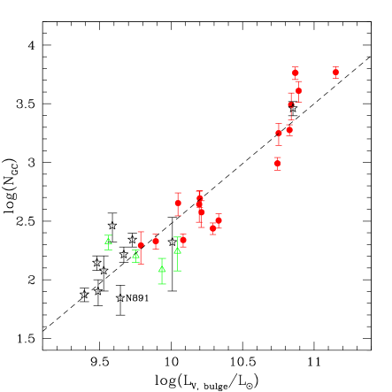
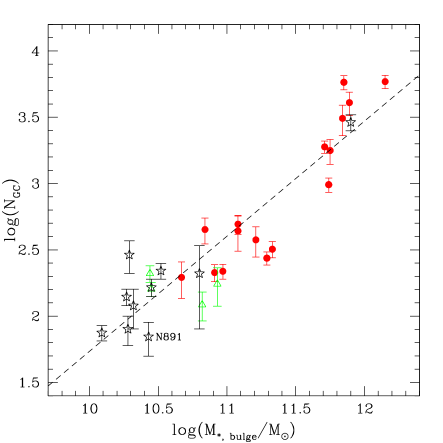
Figure 6.— The log of $N_{\rm GC}$ versus the log of the $V$-band luminosity or stellar mass of the bulge for spiral galaxies or the entire galaxy for elliptical galaxies. The data points represent the 30 galaxies in Tables Exploring the Correlations between Globular Cluster Populations and Supermassive Black Holes in Giant Galaxies and Exploring the Correlations between Globular Cluster Populations and Supermassive Black Holes in Giant Galaxies. The symbols are the same as in Figure 5. The spiral galaxy NGC 891 is not shown in green but may have a pseudobulge. The best-fitting relations are shown as a dashed lines and given in Equations 20 and 21. The relation between $N_{\rm GC}$ and bulge luminosity gives $\chi^{2}/(N-2)$ $=$ 9.2 and the relation between $N_{\rm GC}$ and bulge mass gives $\chi^{2}/(N-2)$ $=$ 11.5.

The quantitative results from the fitting process are mixed. The log of $N_{\rm GC}$ correlates much more closely with the log of the bulge luminosity than it does with total galaxy luminosity. However, the correlation of log($N_{\rm GC}$) with bulge mass is much weaker than that with total galaxy stellar mass. The best-fitting lines to the 30 data points in Figure 6 are

$$\rm{{log\frac{L_{\rm V,bulge}}{L_{\odot}}=(10.22\pm 0.01)+(0.98\pm 0.02)log\frac{N_{GC}}{500}}}$$ (20)

and

$$\rm{{log\frac{M_{*,bulge}}{M_{\odot}}=(11.11\pm 0.01)+(1.15\pm 0.03)log\frac{N_{GC}}{500}}}$$ (21)

which translate to the proportionalities $N_{\rm GC}$ $\propto$ $(L_{\rm V,bulge}$/$L_{\odot})^{1.02}$ and $N_{\rm GC}$ $\propto$ $(M_{*,bulge}$/$M_{\odot})^{0.87}$. The fit of log($N_{\rm GC}$) vs. bulge luminosity yields $\chi^{2}$/$(N-2)$ $=$ 9.2 and $\epsilon_{0}$ $=$ 0.17 dex, whereas the linear fit of log($N_{\rm GC}$) vs. bulge mass gives $\chi^{2}$/$(N-2)$ $=$ 11.5 and $\epsilon_{0}$ $=$ 0.23 dex. By these measures, the tightest correlation of log($N_{\rm GC}$) with any of the galaxy properties examined here is still the correlation with galaxy stellar mass, shown in the right-hand panel of Figure 5 and given in Equation 19.

One might assume that if it is the red, metal-rich GCs that are associated with a galaxy’s spheroidal component, then perhaps the numbers of red GCs will better correlate with bulge luminosity or mass. Including only the red GCs in log($N_{\rm GC}$) and fitting the log of the bulge luminosity or mass produces linear relations with the same slope (within the errors) as those in Equations 20 and 21, but larger $\chi^{2}$ and $\epsilon_{0}$ values. In fact, I also tried executing the fits counting only the blue GCs in each galaxy and found that counting the blue GCs produces a better-quality fit than counting only the red ones. Still, using the total number of GCs produces the best results in terms of $\chi^{2}$ and $\epsilon_{0}$.

To summarize, the relationship between $N_{\rm GC}$ and galaxy mass, or even with bulge luminosity or mass, for the 30 galaxies in this sample yields reduced $\chi^{2}$ values that are smaller than or comparable to the smallest reduced $\chi^{2}$ values yielded by the $N_{\rm GC}$$-$$M_{\rm SMBH}$ fits in Section 3.1. Furthermore, the intrinsic scatter is much smaller for the fits explored in this section ($\epsilon_{0}$ $\sim$ 0.1$-$0.2 dex) than for either the $N_{\rm GC}$$-$$M_{\rm SMBH}$ or the M$-$$\sigma$ relations (both of which have $\epsilon_{0}$ ${}_{>}\atop{{}^{\sim}}$0.4 dex). This seems to imply that the relationship between $N_{\rm GC}$ and the luminosity or mass of the host galaxy is the more fundamental one, and that the observed correlation between $N_{\rm GC}$ and SMBH mass results from both of these quantities being correlated with galaxy mass. As noted earlier, Snyder et al. (2011) came to a similar conclusion based on their analysis of the residuals in the relation between $N_{\rm GC}$ and $M_{\rm SMBH}$ for a sample of elliptical galaxies drawn from BT10 and HH11. The result here is therefore not unexpected since — as the previous papers on this topic (BT10, HH11, and Snyder et al. 2011) have all noted — it seems highly unlikely that the GCs in a galaxy will have some sort of direct causal link to the SMBH located in the galaxy center.

It is relevant to discuss here a recent paper by Sadoun & Colin (2012) that examined other correlations between GC systems and SMBH masses. For a sample of twelve giant spiral, S0, and elliptical galaxies, Sadoun & Colin (2012) find a correlation between the projected velocity dispersion of the GC system ($\sigma_{\rm GC}$) and the SBMH mass that is as tight as the $M$-$\sigma$ relation for those twelve galaxies. In the discussion section of their paper, Sadoun & Colin point out that their observational results might be understood in the context of recent numerical simulations of galaxy formation done by Jahnke & Maccio (2011). Jahnke & Maccio simulate the hierarchical assembly and merger history of dark matter halos over cosmic time, with added recipes for star formation, black hole accretion, and bulge evolution in the simulated galaxies. They then examine the scaling relation between $M_{\rm SMBH}$ and bulge mass that is produced in the resultant galaxies at $z$$=$0. Their conclusion is that correlations between SMBH mass and bulge mass (or velocity dispersion as a proxy for mass) do not require a direct physical link, but rather can arise through normal galaxy merging in a $\Lambda$CDM universe that occurs over the course of a giant galaxy’s history, from high-redshift until $z$$=$0. In Jahnke & Maccio’s simulations, the scaling relations are a natural outcome of the simultaneous build-up of both the central black hole and the galaxy’s stellar component by major galaxy mergers. Jahnke & Maccio state that, “we in principle expect a correlation with $M_{\rm SMBH}$ for any (mass) parameter that is subject to the same $\Lambda$CDM assembly chain”, including correlations between GC populations and $M_{\rm SMBH}$. Sadoun & Colin (2012) point out that this could provide an explanation for their observed $M_{\rm SMBH}$ and $\sigma_{\rm GC}$ results, and likewise it seems to provide a broad context within which we might understand the correlations between the various parameters presented in the current paper.

3.6. Deriving an $M$-$\sigma$ Relation for the Wide-Field GC System Survey Galaxy Sample

One last piece of analysis that can be done with the data set compiled here is to calculate predicted SMBH masses for the giant spiral and elliptical galaxies in Table Exploring the Correlations between Globular Cluster Populations and Supermassive Black Holes in Giant Galaxies. These ten galaxies have well-measured $N_{\rm GC}$ values from my wide-field survey but do not yet have measured masses in the literature for the SMBH that presumably exists in each of their central regions. Nine of the ten galaxies in Table Exploring the Correlations between Globular Cluster Populations and Supermassive Black Holes in Giant Galaxies are spiral galaxies and one (NGC 4406) is a massive Virgo Cluster elliptical. Consequently it seems appropriate to derive $M_{\rm SMBH}$ from the relationship between $N_{\rm GC}$ and $M_{\rm SMBH}$ given in Equation 9, i.e., the linear relation based on the full sample of elliptical, S0, and spiral galaxies analyzed in Section 3.1 and listed in Table Exploring the Correlations between Globular Cluster Populations and Supermassive Black Holes in Giant Galaxies, rather than using the relation derived from only the E/S0 galaxies (Equation 8). The calculated SMBH masses are listed in column (2) of Table Exploring the Correlations between Globular Cluster Populations and Supermassive Black Holes in Giant Galaxies. The errors on the masses are computed by determining the predicted SMBH mass for the upper and lower end of the possible $N_{\rm GC}$ values. For example, $N_{\rm GC}$ for the spiral galaxy NGC 1055 is 220$\pm$30, so the uncertainties in $M_{\rm SMBH}$ reflect the possible range of SMBH values if $N_{\rm GC}$ is 220$-$30$=$190 or 220$+$30$=$250. Published measurements of the central velocity dispersion for nine of the ten galaxies are given in the third column of the table. One galaxy (NGC 7339) apparently does not have a published velocity dispersion, so its SMBH mass is listed in the table but it is excluded from the rest of the analysis in this section.

Figure 7 shows the nine galaxies from Table Exploring the Correlations between Globular Cluster Populations and Supermassive Black Holes in Giant Galaxies with predicted SMBH masses and measured velocity dispersions, added to the $M-\sigma$ plot shown earlier in this paper (Figure 2). As before, the red filled circles are classical-bulge galaxies and the green open triangles are pseudobulge galaxies. The open stars are the nine new galaxies from the wide-field GC system survey. The two lines are the same as those shown in the first $M-\sigma$ plot: the solid line is the best-fitting $M-\sigma$ relation given in Equation 10 and the dotted line is the best-fitting $M-\sigma$ relation published in BT10.

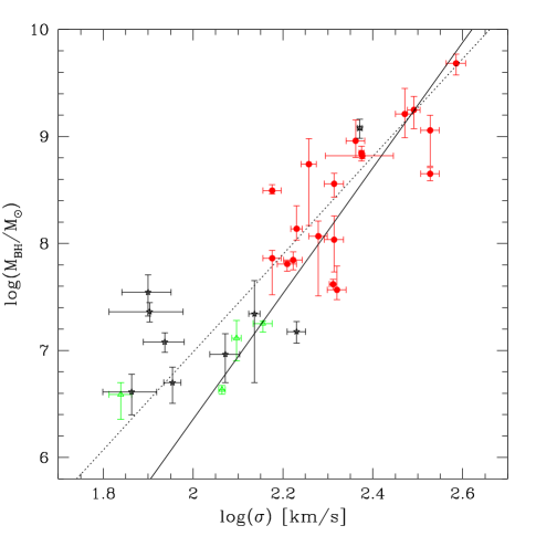
Figure 7.— The log of the measured or predicted SMBH mass versus the log of the central velocity dispersion for the 30 giant galaxies in Tables Exploring the Correlations between Globular Cluster Populations and Supermassive Black Holes in Giant Galaxies and Exploring the Correlations between Globular Cluster Populations and Supermassive Black Holes in Giant Galaxies. As in previous figures, galaxies from Table Exploring the Correlations between Globular Cluster Populations and Supermassive Black Holes in Giant Galaxies are plotted with red filled circles (classical bulges) or green open triangles (pseudobulges) and the $M_{\rm SMBH}$ data plotted are measured values. Open stars denote galaxies from Table Exploring the Correlations between Globular Cluster Populations and Supermassive Black Holes in Giant Galaxies and the $M_{\rm SMBH}$ values are predicted based on the number of GCs in the galaxy and Equation 9. The lines are the same as those plotted in the earlier version of this figure, Figure 2: the solid line is the best-fitting line for the 20 galaxies in Table Exploring the Correlations between Globular Cluster Populations and Supermassive Black Holes in Giant Galaxies and the dotted line is the $M$-$\sigma$ relation from BT10.

Most of the galaxies from the wide-field survey do seem to follow the general relationship between $M_{\rm SMBH}$ and velocity dispersion shown by the two lines. If one adds the data points for these nine galaxies to the data points from Table Exploring the Correlations between Globular Cluster Populations and Supermassive Black Holes in Giant Galaxies and fits a linear relation to the 29 points, the result is a line with the same slope and intercept (5.88$\pm$0.19 and 8.19$\pm$0.03, respectively) within the errors as those of Equation 10, and similar reduced $\chi^{2}$ values ($\chi^{2}$/$(N-4)$ $=$ 12.5 and $\chi^{2}$/$(N-2)$ $=$ 11.6). On the other hand, a few spiral galaxies from the survey — namely, NGC 1055, NGC 3556, and to a lesser extent NGC 4013 — deviate noticeably from the relations in that they have very large $M_{\rm SMBH}$ values for their measured velocity dispersions. One relevant question to ask is: do these galaxies have large predicted SMBH masses because they have anomalously large GC populations? The answer is no: all three of these galaxies have the expected number of GCs based on their stellar mass, i.e., they are not outliers on the $N_{\rm GC}$ versus mass plot (see Figure 5 and the data in Table Exploring the Correlations between Globular Cluster Populations and Supermassive Black Holes in Giant Galaxies). What the data seem to be indicating instead is that $N_{\rm GC}$ is not a particularly good predictor of SMBH mass for some galaxies. The three galaxies that deviate most strongly in the $M-\sigma$ plot are all spiral galaxies. HH11 pointed out that the total number of GCs in the Milky Way was also not a good predictor of its SMBH mass; that is, it deviated strongly from their best-fitting $N_{\rm GC}$$-$$M_{\rm SMBH}$ relation and Figure 1 shows that it deviates from the relation derived here.

The one additional elliptical galaxy from the wide-field survey is NGC 4406, which appears at $log(M_{\rm BH}/M_{\odot})$ $\sim$ 9.1 and $log(\sigma)$ $\sim$ 2.4 in Figure 7. The spiral galaxies all have relatively low $M_{\rm SMBH}$ and velocity dispersion values and lie in the lower left region of the figure. If one considers only the spiral galaxies from the survey, it appears that they actually do not seem to follow an $M-\sigma$ relation and it is really the data point for NGC 4406 that is driving the agreement between the new data and the original best-fitting $M-\sigma$ line. In fact, excluding NGC 4406 from the sample and fitting a line to the other eight data points from the wide-field survey yields a line with zero slope within the errors:

$${\rm{log\frac{M_{\rm SMBH}}{M_{\odot}}=(7.19\pm 0.23)+(0.17\pm 0.80)log\frac{\sigma}{200~{}km~{}s^{-1}}}}$$ (22)

Although it is not entirely obvious what this means, what it seems to suggest is that, again, $N_{\rm GC}$ may not be an accurate predictor of SMBH mass, at least not for spiral galaxies; if there were a tight correlation between the two quantities, one might expect the spiral galaxies to follow the expected $M-\sigma$ relation more closely. A larger sample of galaxies with well-determined values of $N_{\rm GC}$, $M_{\rm SMBH}$, bulge velocity dispersion, and bulge classification would presumably help to clarify these issues.

4. Summary

I have assembled a sample of 20 giant galaxies with both measured SMBH masses and reliable estimates of $N_{\rm GC}$ and GC color fractions based on high-quality wide-field imaging data. The sample includes eight galaxies from my ongoing GC system survey, four galaxies from the ACSVCS survey (Peng et al. 2008), two galaxies from a Gemini study by Faifer et al. (2011), and six galaxies from various studies in the literature. Half of the galaxies in the sample are ellipticals, eight are S0 galaxies, and two are spiral galaxies (the Milky Way and M31). Four of the galaxies may possess pseudobulges according to previous studies of their light profiles and/or kinematics. The sample of 20 galaxies is used to explore correlations between the galaxies’ GC populations and the masses of their central SMBHs. The main findings of this investigation are as follows:

1. The E/S0 galaxies in the sample follow a relation between the log of $N_{\rm GC}$ and the log of the SMBH mass of the form:

   $$\rm{{log\frac{M_{\rm SMBH}}{M_{\odot}}=(8.04\pm 0.03)+(1.22\pm 0.06)log\frac{N_{GC}}{500}}}$$ (23)

   When the two spiral galaxies are included in the sample, the slope and intercept of the relation become 1.52$\pm$0.06 and 7.91$\pm$0.03, respectively. The coefficients of the best-fitting relation for E/S0 galaxies agree within the errors with those of the corresponding relation for early-type galaxies from BT10 (who found a slope of 1.08$\pm$0.04 and an intercept of 8.14$\pm$0.04) and the relation for elliptical galaxies from HH11 (who derived a slope of 0.98$\pm$0.10 and an intercept of 8.30$\pm$0.29).

2. The $M$-$\sigma$ relation for the 20 galaxies in the sample agrees with those in the recent literature within the errors. Three of the four galaxies with pseudobulges (including the Milky Way) closely follow the best-fitting linear relation defined by the classical-bulge galaxies.

3. The numbers of blue, metal-poor GCs in the galaxies yield a slightly smaller reduced $\chi^{2}$ than the numbers of red, metal-rich GCs, although this small difference is probably not statistically significant. In the current picture of galaxy and GC system formation, metal-poor GCs originate in the earliest epoch of galaxy assembly. If metal-poor GC populations were actually more tightly correlated to the SMBH masses in the host galaxies, this might imply that the correlation between $N_{\rm GC}$ and $M_{\rm SMBH}$ is put in place early in the history of the galaxy and does not depend strongly on the occurrence of major merger events later.

4. When the galaxy sample is divided according to Hubble type, the elliptical galaxies retain the tight correlation between $N_{\rm GC}$ and SMBH mass seen in the full sample, whereas the S0 galaxies show more scatter. This is similar to the result in HH11, who found that the S0 galaxies show a large dispersion in black hole mass for a given $N_{\rm GC}$. The four galaxies that may have pseudobulges also seem to show increased scatter compared to the elliptical and classical-bulge galaxies. However, the number of pseudobulge galaxies in the sample is small so it is not clear whether or not the latter trend is real and therefore implies something about how SMBHs grow.

5. Ten more galaxies from my wide-field GC system survey were used to supplement the original sample and explore correlations between $N_{\rm GC}$ and other galaxy properties. The strongest correlation with the smallest intrinsic scatter is a correlation between the number of GCs and the total stellar mass of the host galaxy. In general the correlations between $N_{\rm GC}$ and galaxy mass and luminosity or bulge mass and luminosity are much tighter than any of the $N_{\rm GC}$$-$$M_{\rm SMBH}$ correlations for this sample. This seems to confirm the idea that the observed connection between $N_{\rm GC}$ and $M_{\rm SMBH}$ in giant galaxies is a consequence of the connection between both of these quantities and the galaxy potential.

6. Finally, the $N_{\rm GC}$$-$$M_{\rm SMBH}$ relation derived here is used to calculate predicted SMBH masses for the ten additional galaxies with measured $N_{\rm GC}$ from the wide-field survey but without existing $M_{\rm SMBH}$ measurements in the literature. The single elliptical galaxy in this subsample lies close to the expected $M-\sigma$ relation, but the spiral galaxies show larger scatter, suggesting that $N_{\rm GC}$ is not a reliable predictor of SMBH mass for some galaxies.
   

Table 1Giant Galaxies with Measured SMBH Masses and Global GC System Properties

Name	Type	$M_{BH}$	Ref	$\sigma$	$M_{V}$	Dist	$N_{\rm GC}$	$S_{N}$	$T$	$f_{\rm blue}$	Ref
		($M_{\odot}$)		(km/s)		(Mpc)
N821	E6	3.7($+$2.5,$-$0.7)x107	12	209$\pm$10	-21.0	22.4	320$\pm$45	1.3$\pm$0.2	1.5$\pm$0.2	0.70	22
N1399	E1pec	1.1($+$0.4,$-$0.6)x109	12	337$\pm$16	-22.3	18.5	5800$\pm$700	7.0$\pm$0.8	8.2$\pm$1.0	0.60	3,5
		4.5($+$0.6,$-$0.6)x108
N3379	E1	1.1($+$0.7,$-$0.5)x108	7,12	206$\pm$10	-20.9	10.6	274$\pm$31	1.2$\pm$0.3	1.4$\pm$0.3	0.70	20
		3.6($+$0.9,$-$0.9)x108
N4374	E1	1.6($+$1.2,$-$0.6)x109	12	296$\pm$14	-22.1	18.4	1775$\pm$381	2.7$\pm$0.6	3.1$\pm$0.7	0.59	10
N4472	E2	1.8($+$0.6,$-$0.6)x109	8	310$\pm$10	-23.1	16.7	5870$\pm$680	3.6$\pm$0.6	4.2$\pm$0.6	0.60	19
N4473	E5	1.2($+$0.4,$-$0.8)x108	12	190$\pm$9	-20.7	15.3	376$\pm$97	2.0$\pm$0.5	2.3$\pm$0.6	0.57	17
N4564	E6	6.4($+$0.4,$-$0.9)x107	12	162$\pm$8	-19.9	15.8	213$\pm$31	2.2$\pm$0.3	2.6$\pm$0.4	0.62	17
N4649	E2	4.8($+$1.1,$-$1.1)x109	21	385$\pm$19	-22.4	16.8	4073$\pm$820	4.5$\pm$0.9	5.2$\pm$1.1	0.52	6
N5128	Epec	3.1($+$0.4,$-$0.2)x108	12	150$\pm$7	-22.0	4.6	980$\pm$120	1.5$\pm$0.2	1.8$\pm$0.2	0.53	15
		7.3($+$1.4,$-$3.9)x107
N5813	E1-2	7.0($+$1.1,$-$1.1)x108	11	237$\pm$3	-22.3	32.2	3100$\pm$800	3.9$\pm$0.9	4.5$\pm$1.1	0.57	13
N1023	SB0	4.2($+$0.5,$-$0.5)x107	11	205$\pm$4	-21.1	11.4	494$\pm$80	1.7$\pm$0.3	2.7$\pm$0.4	0.58	23
N3115	S0	9.1($+$5.1,$-$2.8)x108	12	230$\pm$11	-21.1	9.7	439$\pm$130	1.6$\pm$0.3	2.4$\pm$0.7	0.52	6
N3384	SB0	1.8($+$0.1,$-$0.3)x107	12	143$\pm$7	-20.5	11.6	122$\pm$30	0.8$\pm$0.2	1.2$\pm$0.4	0.60	13
N4350	S0	5.5($+$4.0,$-$4.0)x108	11	181$\pm$7	-20.1	16.5	196$\pm$60	1.8$\pm$0.5	2.7$\pm$0.8	0.71	17
N4459	S0	7.0($+$1.3,$-$1.3)x107	12	167$\pm$8	-20.9	16.1	218$\pm$28	1.0$\pm$0.1	1.5$\pm$0.2	0.52	17
N4594	S0/Sa	6.6($+$0.4,$-$0.4)x108	16	238$\pm$41	-22.4	9.8	1890$\pm$200	2.1$\pm$0.3	3.2$\pm$0.5	0.63	20
N7332	S0pec	1.3($+$0.6,$-$0.5)x107	12	125$\pm$3	-20.8	23.0	175$\pm$56	0.9$\pm$0.3	1.4$\pm$0.4	0.57	23
N7457	S0	3.9($+$1.1,$-$1.6)x106	12	69$\pm$4	-19.5	13.2	210$\pm$30	3.1$\pm$0.7	4.8$\pm$1.1	0.58	14
Milky Way	Sbc	4.3($+$0.4,$-$0.4)x106	9	116$\pm$2	-21.3	0.0083	160$\pm$20	0.5$\pm$0.1	1.1$\pm$0.1	0.70	1
M31	Sb	1.4($+$0.9,$-$0.3)x108	4	170$\pm$5	-21.8	0.8	450$\pm$100	0.9$\pm$0.2	1.6$\pm$0.4	0.72	1,2,18

Note. — Morphological types are from the NASA/IPAC Extragalactic Database (NED), with three exceptions. NED lists NGC 5128 as an “S0 pec” or “E/S0”, but studies of this galaxy’s properties and stellar populations (e.g., Hui et al. 1993, Peng et al. 2004, Harris et al. 2004) describe it as an elliptical. NGC 4594 is often classified as an Sa but it has a bulge fraction of $B/T$$=$0.86 (Kent 1988) and broadband colors like an S0, so I list it here as “S0/Sa”. The Milky Way is listed as an Sbc, which is the classification commonly used in the literature (e.g., Ashman & Zepf 1998).

References. — (1) Ashman & Zepf 1998; (2) Barmby et al. 2000; (3) Bassino et al. (2006); (4) Bender et al. 2005; (5) Dirsch et al. 2003; (6) Faifer et al. 2011; (7) Gebhardt et al. 2000a; (8) Gebhardt et al. 2012, in preparation; (9) Gillessen et al. 2009; (10) Gomez & Richtler 2004; (11) Graham 2008; (12) Gultekin et al. 2009; (13) Hargis & Rhode 2012; (14) Hargis et al. 2011; (15) Harris et al. 2004; (16) Jardel et al. 2011; (17) Peng et al. 2008; (18) Perrett et al. (2002); (19) Rhode & Zepf 2001; (20) Rhode & Zepf 2004; (21) Shen & Gebhardt 2010; (22) Spitler et al. 2008; (23) Young, Dowell, & Rhode 2012.

Table 2Results of Fitting Process for $N_{\rm GC}$ and $M_{\rm SMBH}$ Data

Sample	$N_{\rm points}$	$\alpha$	$\beta$	$\chi^{2}$/$(N-4)$	$\chi^{2}$/$(N-2)$	$\epsilon_{0}$
E/S0s	21	8.04$\pm$0.03	1.22$\pm$0.06	10.4	9.3	0.45
All	23	7.91$\pm$0.03	1.52$\pm$0.06	12.4	11.2	0.50
E/S0s, blue GCs	21	8.32$\pm$0.03	1.23$\pm$0.06	10.6	9.5	0.48
E/S0s, red GCs	21	8.52$\pm$0.03	1.20$\pm$0.05	11.0	9.8	0.51
Es	13	8.17$\pm$0.04	0.95$\pm$0.07	9.4	7.7	0.37
S0s (with N4594)	8	7.98$\pm$0.05	1.63$\pm$0.14	16.2	10.8	0.70
S0s (without N4594)	7	10.62$\pm$2.52	10.21$\pm$5.46	9.8	5.9	0.75

Note. — For the fits between $N_{\rm GC}$ and $M_{\rm SMBH}$, the form of the linear relation is log$\frac{M_{\rm SMBH}}{M_{\odot}}$ = $\alpha$ + $\beta$log$\frac{N_{GC}}{500}$. Values of $\epsilon_{0}$ in column (7) are derived by adding $\epsilon_{0}$ in quadrature to the errors on the data points.

Table 3Giant Galaxies with Measured GC System Properties from the Wide-Field Survey and Predicted SMBH Masses

Name	Type	Predicted $M_{BH}$	$\sigma$	$M_{V}$	Distance	$N_{\rm GC}$	$S_{N}$	$T$	$f_{\rm blue}$	Ref
		($M_{\odot}$)	(km/s)		(Mpc)
N4406	E3	1.2($+$0.2,$-$0.2)x109	235$\pm$3	-22.3	16.7	2900$\pm$400	3.5$\pm$0.5	4.1$\pm$0.6	0.62	3
N891	Sb	4.1($+$1.9,$-$1.6)x106	73$\pm$10	-20.8	8.4	70$\pm$20	0.3$\pm$0.1	0.6$\pm$0.3	0.50	1
N1055	Sb	2.3($+$0.5,$-$0.5)x107	80$\pm$15	-21.0	16.3	220$\pm$30	0.9$\pm$0.2	1.7$\pm$0.5	0.59	5
N2683	Sb	9.2($+$5.1,$-$4.2)x106	118$\pm$9	-20.5	7.7	120$\pm$40	0.8$\pm$0.4	1.4$\pm$0.7	0.68	4
N3556	Sc	3.5($+$1.6,$-$1.4)x107	79$\pm$10	-21.2	12.4	290$\pm$80	0.9$\pm$0.4	2.2$\pm$0.9	0.64	4
N4013	Sb	1.2($+$0.3,$-$0.2)x107	86$\pm$9	-20.4	15.1	140$\pm$20	1.0$\pm$0.2	1.9$\pm$0.5	0.74	1
N4157	Sb	5.0($+$2.0,$-$1.8)x106	90$\pm$4	-20.4	14.7	80$\pm$20	0.6$\pm$0.3	1.1$\pm$0.6	0.55	4
N7331	Sb	2.2($+$2.3,$-$1.7)x107	137$\pm$4	-21.7	13.1	210$\pm$130	0.5$\pm$0.3	0.8$\pm$0.7	0.50	4
N7339	Sbc	4.5($+$0.9,$-$0.9)x106	…	-20.4	22.4	75$\pm$10	0.5$\pm$0.2	1.5$\pm$0.5	0.60	5
N7814	Sab	1.5($+$0.4,$-$0.3)x107	170$\pm$8	-20.4	13.2	165$\pm$25	1.3$\pm$0.4	2.2$\pm$0.8	0.58	2

Note. — Morphological types are from the NASA/IPAC Extragalactic Database (NED).

References. — (1) Rhode, Windschitl, & Young 2010; (2) Rhode & Zepf 2003; (3) Rhode & Zepf 2004; (4) Rhode et al. 2007; (5) Young, Dowell, & Rhode 2012.

References

- Alves-Brito et al. (2011) Alves-Brito, A., Hau, G.K.T., Forbes, D.A., Spitler, L.R., Strader, J., Brodie, J.P., & Rhode, K.L. 2011, MNRAS, 417, 1823
- Andrae et al. (2010) Andrae, R., Schulze-Hartung, T., & Melchior, P. 2010, arXiv:1012.3754
- Ashman & Zepf (1992) Ashman, K.M., & Zepf, S.E. 1992, ApJ, 384, 50
- Ashman & Zepf (1998) Ashman, K.M., & Zepf, S.E. 1998, Globular Cluster Systems (Cambridge: Cambridge University Press)
- Barmby et al. (2000) Barmby, P., Huchra, J.P., Brodie, J.P., Forbes, D.A., Schroder, L.L., & Grillmair, C.J. 2000, AJ, 119, 727
- Barmby et al. (2001) Barmby, P., Huchra, J.P., Brodie, J.P. 2001, AJ, 121, 1482
- Baum (1955) Baum, W.A. 1955, PASP, 67, 328
- Bassino et al. (2006) Bassino, L.P., Faifer, F.R., Forte, J.C., Dirsch, B., Richtler, T., Geisler, D., & Schuberth, Y. 2006, A&A, 451, 789
- Bastian et al. (2006) Bastian, N., Saglia, R.P., Goudfrooij, P., Kissler-Patig, M., Maraston, C., Schweizer, F., & Zoccali, M. 2006, å, 448, 881
- Beasley et al. (2002) Beasley, M.A., Baugh, C.M., Forbes, D.A., Sharples, R.M., & Frenk, C.S. 2002, MNRAS, 333, 383
- Beasley et al. (2008) Beasley, M.A., Bridges, T., Peng, E., Harris, W.E., Harris, G.L.H., Forbes, D.A., & Mackie, G. 2008, MNRAS, 386, 1443
- Bender et al. (2005) Bender, R. et al. 2005, ApJ, 631, 280
- Binney & Merrifield (1998) Binney, J. & Merrifield, M. 1998, Galactic Astronomy (Princeton: Princeton Univ. Press), p. 220
- Brodie & Strader (2006) Brodie, J.P. & Strader, J. 2006, ARA&A, 44, 193
- Burkert & Silk (2001) Burkert, A. & Silk, J. 2001, ApJ, 554, 151
- Burkert & Tremaine (2010) Burkert, A. & Tremaine, S. 2010, ApJ, 720, 516
- Côté et al. (1998) Côté, P., Marzke, R.O., & West, M.J. 1998, ApJ, 501, 554
- Côté et al. (2000) Côté, P., Marzke, R.O., & West, M.J., & Minniti, D. 2000, ApJ, 533, 869
- Côté et al. (2004) Côté, P., Blakeslee, J.P., Ferrarese, L., Jordan, A., Mei, S., Merritt, D., Milosavijevic, M., Peng, E.W., Tonry, J.L., & West, M.J. 2004, ApJS, 153, 223
- Dawe & Dickens (1976) Dawe, J.A. & Dickens, R.J. 1976, Nature, 263, 395
- de Jong et al. (2008) de Jong, R. S., Radburn-Smith, D. J., & Sick, J. N. 2009, in IAU Symp. 254, The Galaxy Disk in Cosmological Context, ed. J. Andersen, J. Bland-Hawthorn, & B. Nordstrom (Cambridge: Cambridge Univ. Press), 19
- de Vaucouleurs et al. (1991) de Vaucouleurs, G., de Vaucouleurs, A., Corwin Jr., H.G., Buta, R.J., Paturel, G., & Fouque, P. 1991, Third Reference Catalogue of Bright Galaxies (New York: Springer)
- Di Matteo et al. (2005) Di Matteo, T., Springel, V., & Hernquist, L. 2005, Nature, 433, 604
- Dirsch et al. (2003) Dirsch, B., Richtler, T., Geisler, D., & Forte, J.C., Bassino, L.P., & Gieren, W.P. 2003, AJ, 125, 1908
- Dotter et al. (2010) Dotter, A. et al. 2010, ApJ, 708, 698
- Faber & Jackson (1976) Faber, S.M. & Jackson, R.E. 1976, ApJ, 204, 668
- Faifer et al. (2011) Faifer, F.R., Forte, J.C., Norris, M.A., Bridges, T., Forbes, D.A., Zepf, S.E., Beasley, M., Gebhardt, K., Hanes, D.A., & Sharples, R.M. 2011, MNRAS, 416, 155
- Falcon-Barroso et al. (2004) Falcon-Barroso, J., Peletier, R. F., Emsellem, E., Kuntschner, H., Fathi, K., Bureau, M., Bacon, R., Cappellari, M., Copin, Y., Davies, R. L., de Zeeuw, T. 2004, MNRAS, 350, 35
- Fan et al. (2006) Fan, X. et al. 2006, AJ, 131, 1203
- Ferrarese & Ford (2005) Ferrarese, L. & Ford, H. 2005, SSRv, 116, 523
- Ferrarese & Merritt (2000) Ferrarese, L. & Merritt, D. 2000, ApJ, 539, L9
- Fisher & Drory (2008) Fisher, D.B. & Drory, N. 2008, AJ, 136, 773
- Fisher & Drory (2010) Fisher, D.B. & Drory, N. 2010, ApJ, 716, 942
- Forbes & Bridges (2010) Forbes, D.A. & Bridges, T. 2010, MNRAS, 404, 1203
- Forbes et al. (1997) Forbes, D.A., Brodie, J.P., & Grillmair, C.J. 1997, AJ, 113, 1652
- Forbes et al. (2001) Forbes, D.A., Brodie, J.P., & Larsen, S.S. 2001, ApJ, 556, L83
- Gebhardt et al. (2000a) Gebhardt, K., Richstone, D., Kormendy, J., Lauer, T.R., Ajhar, E.A., Bender, R., Dressler, A., Faber, S.M., Grillmair, C., Magorrian, J., & Tremaine, S. 2000a, AJ, 119, 1157
- Gebhardt et al. (2000b) Gebhardt, K., et al. 2000b, ApJ, 539, L13
- Gillessen et al. (2009) Gillessen, S., Eisenhauer, F., Trippe, S., Alexander, T., Genzel, R., Martins, F., & Ott, T. 2009, ApJ, 692, 1075
- Gomez & Richtler (2004) Gomez, M. & Richtler, T. 2004, A&A, 415, 499
- Goudfrooij et al. (2007) Goudfrooij, P., Schweizer, F., Gilmore, D., & Whitmore, B.C. 2007, AJ, 133, 2737
- Graham (2008) Graham, A.W. 2008, PASA, 25, 167
- Graham et al. (2011) Graham, A.W., Onken, C.A., Athanassoula, E., & Combes, F. 2011, MNRAS, 412, 2211
- Graham & Worley (2008) Graham, A.W. & Worley, C.C. 2008, MNRAS, 388, 1708
- Gultekin et al. (2009) Gultekin, K., Richstone, D.O., Gebhardt, K., Lauer, T.R., Tremaine, S., Aller, M.C., Bender, R., Dressler, A., Faber, S.M., Filippenko, A.V., Green, R., Ho, L.C., Kormendy, J., Magorrian, J., Pinkney, J., & Siopis, C. 2009, ApJ, 698, 198
- Hanes (1977) Hanes, D.A. 1977, MmRAS, 84, 45 ‘
- Hargis & Rhode (2012) Hargis, J.R. & Rhode, K.L. 2012, AJ, in press
- Hargis et al. (2011) Hargis, J.R., Rhode, K.L., Strader, J., & Brodie, J.P. 2011, ApJ, 738, 113
- Harris (1981) Harris, W. 1981, ApJ, 251, 497
- Harris (1991) Harris, W. 1991, ARA&A, 29, 543
- Harris & Harris (2011) Harris, G.L.H. & Harris, W.E. 2011, MNRAS, 410, 2347
- Harris et al. (2004) Harris, G.L.H., Harris, W.E., & Geisler, D. 2004, AJ, 128, 723
- Harris & van den Bergh (1981) Harris, W.E. & van den Bergh, S. 1981, AJ, 86, 1627
- Ho et al. (2009) Ho, L., Greene, J.E., Filippenko, A.V., & Sargent, W.L.W. 2009, ApJSS, 183, 1
- Hopkins et al. (2007) Hopkins, P.F., Hernquist, L., Cox, T.J., Robertson, B., & Krause, E. 2007, ApJ, 669, 67
- Howard et al. (2008) Howard, C.D., Rich, M.R., Reitzel, D.B., Koch, A., De Propris, R., & Zhao, H. 2008, ApJ, 688, 1060
- Hui et al. (1993) Hui, X., Ford, H.C., Ciardullo, R., & Jacoby, G.H. 1993, ApJ, 414, 463
- Jahnke & Maccio (2011) Jahnke, K. & Maccio, A.V. 2011, ApJ, 734, 92
- Jardel et al. (2011) Jardel, J.R., Gebhardt, K., Shen, J., Fisher, D.B., Kormendy, J., Kinzler, J., Lauer, T.R., Richstone, D., & Gultekin, K. 2011, ApJ, 739, 21
- Jarrett et al. (2000) Jarrett, T.H., Chester, T., Cutri, R., Schneider, S., Skrutskie, M., & Huchra, J.P. 2000, AJ, 119, 2498
- Jarrett et al. (2003) Jarrett, T.H., Chester, T., Cutri, R., Schneider, S.E., & Huchra, J.P. 2003, AJ, 125, 525
- Johansson et al. (2009) Johansson, P.H., Burkert, A., & Naab, T. 2009, ApJ, 707, L184
- Jordan et al. (2007) Jordan, A., McLaughlin, D.E., Cote, P., Ferrarese, L., Peng, E.W., Mei, S., Villegas, D., Merritt, D., Tonry, J.L., & West, M.J. 2007, ApJS, 171, 101
- Kavelaars et al. (2000) Kavelaars, J.J., Harris, W.E., Hanes, D.A., Hesser, J.E., Pritchet, C.J. 2000, ApJ, 533, 125
- Kent (1985) Kent, S.M. 1985, ApJS, 59, 115
- Kent (1988) Kent, S.M. 1988, AJ, 96, 2
- Kormendy (1993) Kormendy, J. 1993, in Galactic bulges: proceedings of the 153rd Symposium of the International Astronomical Union, ed. H. DeJonghe & H.J. Habing (Dordrecht: Kluwer), 209
- Kormendy et al. (2011) Kormendy, J., Bender, R., & Cornell, M.E. 2011, Nature, 469, 374
- Kormendy & Kennicutt (2004) Kormendy, J. & Kennicutt, R.C., Jr. 2004, ARA&A, 42, 603
- Kruijssen et al. (2012) Kruijssen, M.D., Inti Pelupessy, F., Lamers, H.J.G.L.M., Portegies Zwart, S.F., Bastian, N., Icke, V. 2012, MNRAS, 421, 1927
- Kundu & Whitmore (2001) Kundu, A. & Whitmore, B.C. 2001, AJ, 121, 2950
- Kundu & Zepf (2007) Kundu, A. & Zepf, S.E. 2007, ApJ, 660, L109
- Lee et al. (1998) Lee, M.G., Kim, E., & Geisler, D. 1998, AJ, 115, 947
- Mayer et al. (2010) Mayer, L., Kazantzidis, S., Escala, A., & Callegari, S. 2010, Nature, 466, 1082
- Miralda-Escude & Kollmeier (2005) Miralda-Escude, J. & Kollmeier, J. 2005, ApJ, 619, 30
- Moore et al. (2006) Moore, B., Diemand, J., Madau, P., Zemp, M., & Stadel, J. 2006, MNRAS, 368, 563
- Mortlock et al. (2011) Mortlock, S.J. et al. 2011, Nature, 474, 616
- Muratov & Gnedin (2010) Muratov, A.L. & Gnedin, O.Y. 2010, ApJ, 718, 1266
- Omukai et al. (2008) Omukai, K., Schneider, R., & Haiman, Z. 2008, ApJ, 686, 801
- Peng et al. (2004) Peng, E.W., Ford, H.C., & Freeman, K.C. 2004, ApJS, 150, 367
- Peng et al. (2006) Peng, E.W., Jordan, A., Cote, P., Blakeslee, J.P., Ferrarese, L., Mei, S., West, M.J., Merritt, D., Milosavljevic, M., & Tonry, J.L. 2006, ApJ, 639, 95
- Peng et al. (2008) Peng, E.W., Jordan, A., Cote, P., Takamiya, M., West, M.J., Blakeslee, J.P., Chen, C.-W., Ferrarese, L., Mei, S., Tonry, J.L., & West, A.A. 2008, ApJ, 681, 197
- Perrett et al. (2002) Perrett, K.M., Bridges, T.J., Hanes, D.A., Irwin, M.J., Brodie, J.P., Carter, D., Huchra, J.P., & Watson, F.G. 2002, AJ, 123, 2490
- Pinkney et al. (2003) Pinkney, J., Gebhardt, K., Bender, R., Bower, G., Dressler, A., Faber, S.M., Filippenko, A.V., Green, R., Ho, L.C., Kormendy, J., Lauer, T.R., Magorrian, J., Richstone, D., & Tremaine, S. 2003, ApJ, 596, 903
- Press et al. (1992) Press, W. H., Teukolsky, S. A., Vetterling, W. T., & Flannery, B. P. 1992, Numerical Recipes (2d ed.; Cambridge: Cambridge Univ. Press)
- Rhode & Zepf (2001) Rhode, K.L. & Zepf, S.E. 2001, AJ, 121, 210
- Rhode & Zepf (2003) Rhode, K.L. & Zepf, S.E. 2003, AJ, 126, 2307
- Rhode & Zepf (2004) Rhode, K.L. & Zepf, S.E. 2004, AJ, 127, 302
- Rhode et al. (2005) Rhode, K.L., Zepf, S.E., & Santos, M.R. 2005, ApJ, 630, L21
- Rhode et al. (2007) Rhode, K.L., Zepf, S.E., Kundu, A., & Larner, A.N. 2007, AJ, 134, 1403
- Rhode et al. (2010) Rhode, K.L., Windschitl, J.L., & Young, M.D. 2010, AJ, 140, 430
- Robertson et al. (2006) Robertson, B., Hernquist, L., Cox, T.J., Di Matteo, T., Hopkins, P.F., Martini, P., & Springel, V. 2006, ApJ, 641, 90
- Sadoun & Colin (2012) Sadoun, R. & Colin, J. 2012, MNRAS, in press
- Sandage (1961) Sandage, A. 1961, The Hubble Atlas of Galaxies (Washington, D.C.: Carnegie Inst. of Washington)
- Santos (2003) Santos, M.R. 2003, in Extragalactic Globular Cluster Systems, ed. M. Kissler-Patig (New York: Springer-Verlag)
- Schwarzschild et al. (1955) Schwarzschild, M., Searle, L., & Howard, R. 1955, ApJ, 122, 353
- Shen & Gebhardt (2010) Shen, J. & Gebhardt, K. 2010, ApJ, 711, 484
- Shen et al. (2010) Shen, J., Rich, R.M., Kormendy, J., Howard, C.D., De Propris, R., & Kunder, A. 2010, ApJ, 720, L72
- Sheth (2003) Sheth, R.K. 2003, MNRAS, 345, 1200
- Simien & de Vaucouleurs (1986) Simien, F. & de Vaucouleurs, G. 1986, ApJ, 302, 564
- Snyder et al. (2011) Snyder, G.F., Hopkins, P.F., & Hernquist, L. 2011, ApJ, 728, L24
- Spitler & Forbes (2009) Spitler, L.R. & Forbes, D.A. 2009, MNRAS, 392, L1
- Spitler et al. (2008) Spitler, L.R., Forbes, D.A., Strader, J., Brodie, J.P., & Gallagher, J.S. 2008, MNRAS, 385, 361
- Strader et al. (2007) Strader, J., Beasley, M.A., & Brodie, J.P. 2007, AJ, 133, 2015
- Strader et al. (2004) Strader, J., Brodie, J.P., & Forbes, D.A. 2004, AJ, 127, 3431
- Sweigart & Gross (1978) Sweigart, A.V. & Gross, P.G. 1978, ApJS, 36, 405
- Tamura et al. (2006) Tamura, N., Sharples, R. M., Arimoto, N., Onodera, M., Ohta, K., Yamada, Y. 2006, MNRAS, 373, 588
- Tremaine et al. (2002) Tremaine, S., Gebhardt, K., Bender, R., Bower, G., Dressler, A., Faber, S.M., Filippenko, A.V., Green, R., Grillmair, C., Ho, L.C., Kormendy, J., Lauer, T.R., Magorrian, J., Pinkney, J., & Richstone, D. 2002, ApJ, 574, 740
- Tully (1988) Tully, R.B. 1988, Nearby Galaxies Catalog (New York: Cambridge Univ. Press)
- van den Bergh (1993) van den Bergh, S. 1993, ApJ, 411, 178
- Vesperini (2000) Vesperini, E. 2000, MNRAS, 318, 841
- Volonteri & Rees (2006) Volonteri, M. & Rees, M.J. 2006, ApJ, 650, 669
- Whitmore et al. (1995) Whitmore, B.C., Sparks, W.B., Lucas, R.A., Macchetto, F.D., & Biretta, J.A. 1995, ApJ, 454, L73
- Whitmore et al. (2010) Whitmore, B.C., Chandar, R., Schweizer, F., Rothberg, B., Leitherer, C., Rieke, M., Rieke, G., Blair, W.P., Mengel, S., & Alonso-Herrero, A. 2010, AJ, 140, 75
- Young et al. (2012) Young, M.D., Dowell, J.L., & Rhode, K.L. 2012, AJ, 144, 103
- Zepf & Ashman (1993) Zepf, S.E., & Ashman, K.M. 1993, MNRAS, 264, 611
- Zinn (1985) Zinn, R. 1985, ApJ, 293, 424