A Nyström method for the two dimensional
Helmholtz hypersingular equation

Abstract

In this paper we propose and analyze a class of simple Nyström discretizations of the hypersingular integral equation for the Helmholtz problem on domains of the plane with smooth parametrizable boundary. The method depends on a parameter (related to the staggering of two underlying grids) and we show that two choices of this parameter produce convergent methods of order two, while all other stable methods provide methods of order one. Convergence is shown for the density (in uniform norm) and for the potential postprocessing of the solution. Some numerical experiments are given to illustrate the performance of the method.

1 Introduction

In this paper we propose and analyze a discretization of the hypersingular integral equation for the Helmholtz equation on a smooth parametrizable simple curve $\Gamma\subset\mathbb{R}^{2}$:

$$-\partial_{\nu}\int_{\Gamma}\partial_{\nu(\mathbf{y})}H^{(1)}_{0}(k|\cdot-\mathbf{y}|)\phi(\mathbf{y})\mathrm{d}\Gamma(\mathbf{y})=g\quad\mbox{on $\Gamma$.}$$ (1)

Here $H^{(1)}_{0}$ is the Hankel function of the first kind and order zero, $k$ is the wave number, $\partial_{\nu}$ is the normal derivative, and $g$ is data on $\Gamma$. The method is based on some simple ideas:

• The operator is first written as a bilinear integrodifferential form acting on periodic functions

  $$(\psi,\varphi) \longmapsto \int_{0}^{1}\int_{0}^{1}H^{(1)}_{0}(k|\mathbf{x}(s)-\mathbf{x}(t)|)\psi^{\prime}(s)\varphi^{\prime}(t)\mathrm{d}s\mathrm{d}t$$

  $$-k^{2}\int_{0}^{1}\int_{0}^{1}H^{(1)}_{0}(k|\mathbf{x}(s)-\mathbf{x}(t)|)\mathbf{n}(s)\cdot\mathbf{n}(t)\psi(s)\varphi(t)\mathrm{d}s\mathrm{d}t,$$

  $\mathbf{x}=(x_{1},x_{2})$ being a regular parametrization of $\Gamma$, and $\mathbf{n}=(x_{2}^{\prime},-x_{1}^{\prime})$ the outward pointing normal vector.

• The principal part of the bilinear form (the one with the derivatives) is formally approximated with a nonconforming Petrov-Galerkin scheme, using piecewise constant functions on two different uniform grids with the same mesh-size $h$: $\{(j-\frac{1}{2})h\}$ and $\{(j-\frac{1}{2}+\varepsilon)h\}$. Since the derivatives of piecewise constant functions are linear combinations of Dirac delta distributions, that part of the bilinear form is just discretized with the matrix

  $$\mathrm{W}_{i+1,j+1}-\mathrm{W}_{i,j+1}+\mathrm{W}_{i,j}-\mathrm{W}_{i+1,j},$$

  where $\mathrm{W}_{i,j}=H^{(1)}_{0}(k|\mathbf{b}_{i}^{\varepsilon}-\mathbf{b}_{j}|)$, $\mathbf{b}_{i}^{\varepsilon}:=\mathbf{x}((i-{\textstyle\frac{1}{2}}+\varepsilon)h)$, and $\mathbf{b}_{j}:=\mathbf{x}((j-{\textstyle\frac{1}{2}})h)$.

• The second part of the bilinear form (which has a weakly singular logarithmic singularity) is discretized with the same Petrov-Galerkin scheme, using midpoint quadrature to approximate the resulting integrals:

  $$k^{2}H^{(1)}_{0}(k|\mathbf{m}_{i}^{\varepsilon}-\mathbf{m}_{j}|)\mathbf{n}_{i}^{\varepsilon}\cdot\mathbf{n}_{j}$$

  $$\approx k^{2}\int_{(i-\frac{1}{2}+\varepsilon)h}^{(i+\frac{1}{2}+\varepsilon)h}\int_{(j-\frac{1}{2})h}^{(j+\frac{1}{2})h}H^{(1)}_{0}(k|\mathbf{x}(s)-\mathbf{x}(t)|)\mathbf{n}(s)\cdot\mathbf{n}(t)\mathrm{d}s\mathrm{d}t,$$

  where $\mathbf{m}_{i}^{\varepsilon}:=\mathbf{x}((i+\varepsilon)h)$, $\mathbf{n}_{i}^{\varepsilon}:=h\,\mathbf{n}((i+\varepsilon)h)$ and $\mathbf{m}_{j}$ and $\mathbf{n}_{j}$ are similarly defined.

• The right-hand side is tested with piecewise constant functions and then midpoint quadrature is applied to all the resulting integrals.

As can be seen from the above formulas, this method leads to a very simple discretization of (1), requiring no assembly process, no additional numerical integration and no complicated data structures to handle the geometric data.

The use of a two-grid Nyström method for periodic logarithmic integral equations goes back to the work of Jukka Saranen, Ian Sloan and their collaborators [9, 10, 13]. It was then discovered that the values $\varepsilon=\pm 1/6$ provide superconvergent methods (of order two) and that the values $\varepsilon=\pm 1/2$ lead to unstable discretizations. The idea was further exploited in [2], showing that the methods can be used on the weakly singular equations that appear in the Helmholtz equation. The present paper shows how to transfer the same kind of ideas (and, up to a point, the same type of analysis) to the hypersingular integral equation for the Helmholtz equation. The case of the Laplace hypersingular equation is included in the present analysis.

We will show that this discretization of the hypersingular integral operator is stable in the $L^{2}$ norm for the underlying space of piecewise constant functions as long as $\varepsilon\neq\pm 1/2$ (the value $\varepsilon=0$ is excluded as a possibility from the very beginning, since it leads to evaluation of the kernel functions on the singularity). We will also show that $\varepsilon=\pm 1/6$ define methods of order two and that this order is actually attained in a strong $L^{\infty}$ norm. The error analysis will be based on Fourier techniques [1, 9, 11] combined with an already quite extensive library of asymptotic expansions developed by two of the authors of this paper with some other collaborators [2, 4, 5, 6].

In a forthcoming paper [3] we will show how to combine this discretization method for the hypersingular equation with the original method [2, 9, 10, 13] for the single layer operator and with straightforward Nyström discretization of the double layer operator and its adjoint. This results in a compatible and straightforward-to-code fully discrete Calderón Calculus for the two dimensional Helmholtz equation on a finite number of disjoint smooth closed curves. This discretization set has a strong flavor to low order Finite Differences. This might make it an attractive option to build simple code for scattering problems, when the simultaneous use of several boundary integral operators is required.

The paper is structured as follows. In Section 2 we present the method for a class of periodic hypersingular equations that include (1) after parametrization. The method is then reinterpreted as a non-conforming Petrov-Galerkin discretization with numerical quadrature. In Section 3, we introduce the functional frame for the analysis of the method, based on the theory of periodic pseudodifferential operators on periodic Sobolev spaces. In Section 4 we present the stability result of this paper in the form of an infimum-supremum condition. In Sections 5 and 6, we respectively give the consistency and convergence error estimates for the method. Section 7 contains some numerical experiments, while we have gathered in Appendix A the more technical proof of Proposition 12.

2 The equation and the method

We are going to present the method for a hypersingular integral equation associated to the two dimensional equation on a simple smooth curve. The extension to a finite set of non-intersecting smooth curves is straightforward. Since everything can be expressed with periodic integral equations, and the analysis will be carried out at that level of generality, we start this work by presenting the equation in that language.

2.1 A class of integrodifferential operators and its discretization

We consider two logarithmic kernel functions:

$$V_{\ell}(s,t):={\textstyle\frac{\imath}{2\pi}}A_{\ell}(s,t)\log(\sin^{2}\pi(s-t))+K_{\ell}(s,t),\qquad\ell\in\{1,2\},$$ (2)

where $A_{1},A_{2},K_{1},K_{2}\in\mathcal{C}^{\infty}(\mathbb{R}^{2})$ are 1-periodic in both variables and

$$A_{1}(s,s)\equiv\alpha\neq 0.$$ (3)

We consider the associated integral operators

$$\mathrm{V}_{j}\varphi:=\int_{0}^{1}V_{j}(\,\cdot\,,t)\varphi(t)\mathrm{d}t,$$ (4)

and the operator

$$\mathrm{W}:=-\mathrm{D}\mathrm{V}_{1}\mathrm{D}+\mathrm{V}_{2},\qquad\mathrm{D}\varphi:=\varphi^{\prime}.$$ (5)

Let us consider the space of smooth 1-periodic functions $\mathcal{D}:=\{\varphi\in\mathcal{C}^{\infty}(\mathbb{R})\,:\,\varphi(1+\,\cdot\,)=\varphi\}.$ An important hypothesis is injectivity:

$$\varphi\in\mathcal{D},\quad\mathrm{W}\varphi=0\qquad\Longrightarrow\qquad\varphi=0.$$ (6)

As we will see later on, this injectivity condition is enough to prove invertibility of $\mathrm{W}$ in a wide range of Sobolev spaces. Given a smooth 1-periodic function $g$, we look for $\varphi$ such that

$$\mathrm{W}\varphi=g.$$ (7)

The discretization method uses four sets of discretization points. Let $N$ be a positive integer, $h:=1/N$, and

$$s_{i}=(i-{\textstyle\frac{1}{2}})h,\quad t_{i}:=i\,h,\quad s_{i+\varepsilon}:=(i+\varepsilon-{\textstyle\frac{1}{2}})h,\quad t_{i+\varepsilon}:=(i+\varepsilon)h,\quad i\in\mathbb{Z}.$$ (8)

(We will comment on $\varepsilon$ shortly.) The discretization method looks for

$$(\varphi_{0},\ldots,\varphi_{N-1})\in\mathbb{C}^{N}\quad\mbox{such that}\quad\sum_{j=0}^{N-1}W_{ij}^{\varepsilon}\varphi_{j}=hg(t_{i+\varepsilon})\quad i=0,\ldots,N-1,$$ (9)

where

$$W_{ij}^{\varepsilon} := V_{1}(s_{i+1+\varepsilon},s_{j+1})-V_{1}(s_{i+\varepsilon},s_{j+1})-V_{1}(s_{i+1+\varepsilon},s_{j})+V_{1}(s_{i+\varepsilon},s_{j})$$ (10)

$$+h^{2}V_{2}(t_{i+\varepsilon},t_{j}).$$

Substitution of $\varepsilon$ by $\varepsilon+1$ produces the same method. The option $\varepsilon\in\mathbb{Z}$ is not practicable, since it leads to evaluations of the logarithmic kernels in their diagonal singularity. The method for $\varepsilon=1/2$ ( $\varepsilon\in 1/2+\mathbb{Z}$) will not fit in our analysis, that relies on stability properties of an $\varepsilon-$dependent discretization of logarithmic operators that is unstable for $\varepsilon=1/2$. (We will show numerical evidence that the value $\varepsilon=1/2$ is valid though.) All other methods will provide convergent schemes, with two superconvergent cases. Namely, we will see that for smooth enough solutions, we can prove:

$$\max_{j}|\varphi_{j}-\varphi(t_{j})|=\mathcal{O}(h),\qquad\mbox{if }\varepsilon\not\in{\textstyle\frac{1}{2}}\mathbb{Z}$$

(this excludes the non-practicable and unstable cases), and that

$$\max_{j}|\varphi_{j}-\varphi(t_{j})|=\mathcal{O}(h^{2}),\qquad\mbox{if }\varepsilon\in\pm{\textstyle\frac{1}{6}}+\mathbb{Z}.$$

These results will be proved as Theorems 3 and 4 respectively.

2.2 A non-conforming Petrov-Galerkin method

We next give some intuition on how to come up with the method (9)-(10). We can formally rewrite (7) in variational form

$$\int_{0}^{1}\psi^{\prime}(s)(\mathrm{V}_{1}\varphi^{\prime})(s)\mathrm{d}s+\int_{0}^{1}\psi(s)(\mathrm{V}_{2}\varphi)(s)\mathrm{d}s=\int_{0}^{1}\psi(s)g(s)\mathrm{d}s.$$ (11)

Consider now the function $\chi_{i}$ that arises from 1-periodization of the characteristic function of the interval $(s_{i},s_{i+1})=(t_{i}-h/2,t_{i}+h/2)$, that is,

$$\chi_{i}(1+\,\cdot\,)=\chi_{i},\qquad\chi_{i}\big{|}_{(s_{i},s_{i+1})}\equiv 1,\qquad\chi_{i}\big{|}_{[s_{i+1},s_{i+N}]}\equiv 0.$$ (12)

We similarly define the functions $\chi_{i+\varepsilon}$ by periodizing the characteristic functions of the intervals $(s_{i+\varepsilon},s_{i+1+\varepsilon})=(t_{i+\varepsilon}-h/2,t_{i+\varepsilon}+h/2)$. The weak derivatives of these functions can be expressed through the use of Dirac delta distributions. In addition to understanding Dirac deltas as periodic distributions (see Section 3.2), we will admit the action of Dirac deltas on any function that is continuous around the point where the delta is concentrated. At the present stage, we only need to consider the functionals

$$\{\delta_{s_{i}},\varphi\}:=\varphi(s_{i}),\qquad\{\delta_{s_{i+\varepsilon}},\varphi\}:=\varphi(s_{i+\varepsilon}),$$ (13)

acting on any 1-periodic function $\varphi$ that is smooth in a neighborhood of $s_{i}$ and $s_{i+\varepsilon}$. Admitting formally that $\chi_{i}^{\prime}=\delta_{s_{i}}-\delta_{s_{i+1}}$ and $\chi_{i+\varepsilon}^{\prime}=\delta_{s_{i+\varepsilon}}-\delta_{s_{i+1+\varepsilon}}$, we consider a non-conforming Petrov-Galerkin discretization of (11):

$$\varphi_{h}:=\sum_{j=0}^{N-1}\varphi_{j}\chi_{j}\quad\mbox{such that}\quad\sum_{j=0}^{N}W_{ij}^{\varepsilon,\circ}\varphi_{j}=\int_{t_{i+\varepsilon}-\frac{h}{2}}^{t_{i+\varepsilon}+\frac{h}{2}}g(s)\mathrm{d}s,\qquad i=0,\ldots,N-1,$$ (14)

where

$$W_{ij}^{\varepsilon,\circ} := V_{1}(s_{i+1+\varepsilon},s_{j+1})-V_{1}(s_{i+\varepsilon},s_{j+1})-V_{1}(s_{i+1+\varepsilon},s_{j})+V_{1}(s_{i+\varepsilon},s_{j})$$ (15)

$$+\int_{t_{i+\varepsilon}-\frac{h}{2}}^{t_{i+\varepsilon}+\frac{h}{2}}\int_{t_{j}-\frac{h}{2}}^{t_{j}+\frac{h}{2}}V_{2}(s,t)\mathrm{d}s\mathrm{d}t.$$

Note that

$$\sum_{j=0}^{N-1}\Big{(}\int_{t_{i+\varepsilon}-\frac{h}{2}}^{t_{i+\varepsilon}+\frac{h}{2}}\int_{t_{j}-\frac{h}{2}}^{t_{j}+\frac{h}{2}}V_{2}(s,t)\mathrm{d}s\mathrm{d}t\Big{)}\varphi_{j}=\int_{t_{i+\varepsilon}-\frac{h}{2}}^{t_{i+\varepsilon}+\frac{h}{2}}(\mathrm{V}_{2}\varphi_{h})(s)\mathrm{d}s$$

and that the leading term in $W_{ij}^{\varepsilon,\circ}$ can be understood as the action

$$\{\delta_{s_{i+\varepsilon}}-\delta_{s_{i+1+\varepsilon}},\mathrm{V}_{1}(\delta_{s_{j}}-\delta_{s_{j+1}})\}=\{\chi_{i+\varepsilon}^{\prime},\mathrm{V}_{1}\chi_{j}^{\prime}\}.$$ (16)

The method (9)-(10) is recovered if we use midpoint integration for all integrals in (14)-(15).

2.3 Relation to the Helmholtz equation

Let $\mathbf{x}:\mathbb{R}\to\mathbb{R}^{2}$ be a smooth 1-periodic function such that $|\mathbf{x}^{\prime}(s)|\neq 0$ for all $s$, and $\mathbf{x}(s)\neq\mathbf{x}(t)$ if $|s-t|<1$. The range of $\mathbf{x}$ is then a smooth closed curve $\Gamma$ in the plane. Let $\mathbf{n}(t)$ be the outward pointing normal vector at $\mathbf{x}(t)$ with $|\mathbf{n}(t)|=|\mathbf{x}^{\prime}(t)|$. Given a periodic function $\varphi$, we define

$$\mathbb{R}^{2}\setminus\Gamma\ni\mathbf{z}\mapsto U(\mathbf{z}) := \frac{\imath}{4}\int_{0}^{1}\nabla_{\mathbf{y}}H^{(1)}_{0}(k|\mathbf{z}-\mathbf{y}|)\Big{|}_{\mathbf{y}=\mathbf{x}(t)}\cdot\mathbf{n}(t)\,\varphi(t)\mathrm{d}t$$

$$= \frac{\imath k}{4}\int_{0}^{1}H^{(1)}_{1}(k|\mathbf{z}-\mathbf{x}(t)|)\,\frac{(\mathbf{z}-\mathbf{x}(t))\cdot\mathbf{n}(t)}{|\mathbf{z}-\mathbf{x}(t)|}\varphi(t)\mathrm{d}t,$$

where $H^{(1)}_{0}$ and $H^{(1)}_{1}$ are the Hankel functions of the first kind and orders $0$ and $1$ respectively. The function $U$ is an outgoing solution of the Helmholtz equation

$$\Delta U+k^{2}U=0\quad\mbox{in $\mathbb{R}^{2}\setminus\Gamma$},\qquad\qquad\frac{\partial U}{\partial r}-\imath kU=o(r^{-1/2})\quad\mbox{as $r=|\mathbf{z}|\to\infty$},$$ (18)

with the asymptotic limit (the Sommerfeld radiation condition) holding uniformly in all directions: $U$ is the double layer potential with (parametrized) density $\varphi$ (see [7, Section 2.1]). The double layer potential is discontinuous across $\Gamma$ but its normal derivative on $\Gamma$ coincides from both sides. If we define

$$(\mathrm{W}\varphi)(s):=-(\nabla U(\mathbf{x}(s))\cdot\mathbf{n}(s),$$

then,

$$(\mathrm{W}\varphi)(s) = -\frac{\imath}{4}\frac{\mathrm{d}}{\mathrm{d}s}\int_{0}^{1}H^{(1)}_{0}(k|\mathbf{x}(s)-\mathbf{x}(t)|)\varphi^{\prime}(t)\mathrm{d}t$$ (19)

$$-\frac{\imath k^{2}}{4}\int_{0}^{1}H^{(1)}_{0}(k|\mathbf{x}(s)-\mathbf{x}(t)|)\mathbf{n}(s)\cdot\mathbf{n}(t)\,\varphi(t)\mathrm{d}t.$$

This is just the parametrized form of a well known formula: see [12, Theorem 3.3.22] or [8, Exercise 9.6]. Using the asymptotic behavior of Hankel functions close to the singularity, it can be shown that the weakly singular kernel $H^{(1)}_{0}(k|\mathbf{x}(s)-\mathbf{x}(t)|)$ can be decomposed as in (2) with $A_{1}(s,s)\equiv\imath/2$ (see (3)). Therefore, the operator $\mathrm{W}$ in (19) fits in the frame of (5).

The operator $\mathrm{W}$ satisfies the injectivity condition (6) if and only if $k^{2}$ is not a Neumann eigenvalue of the Laplace operator in the interior of $\Gamma$ [7, Section 2.1]. In those cases, the solution of the interior-exterior Helmholtz equation (18) with Neumann boundary condition $\partial_{\nu}u=f$ can be represented with the double layer ansatz (2.3), $\varphi$ being a solution of equation (7) with $g:=-f\circ\mathbf{x}$. If we then apply the discretization (9)-(10), we can construct a fully discrete potential representation, when we substitute $\varphi$ by $\varphi_{h}:=\sum_{j=0}^{N-1}\varphi_{j}\chi_{j}$ in (2.3) and apply midpoint integration:

$$U_{h}(\mathbf{z}):=\frac{\imath k}{4}\,h\,\sum_{j=0}^{N-1}H^{(1)}_{1}(k|\mathbf{z}-\mathbf{x}(t_{j})|)\,\frac{(\mathbf{z}-\mathbf{x}(t_{j}))\cdot\mathbf{n}(t_{j})}{|\mathbf{z}-\mathbf{x}(t_{j})|}\,\varphi_{j}.$$ (20)

3 Functional frame

3.1 Asymptotics of hypersingular operators

Consider the space $\mathcal{D}$ of periodic $\mathcal{C}^{\infty}$ complex valued functions of one variable, endowed with the metric that imposes uniform convergence of all derivatives [11, Section 5.2]. A periodic distribution is an element of $\mathcal{D}^{\prime}$, the dual space of $\mathcal{D}$. Given $u\in\mathcal{D}^{\prime}$, we consider its Fourier coefficients

$$\widehat{u}(m):=\langle u,\phi_{m}\rangle_{\mathcal{D}^{\prime}\times\mathcal{D}},\qquad\phi_{m}(t):=\exp(2\pi\imath mt),\qquad m\in\mathbb{Z}.$$ (21)

The periodic Sobolev space of order $r\in\mathbb{R}$ is

$$H^{r}:=\{u\in\mathcal{D}^{\prime}\,:\,\|u\|_{r}<\infty\},\qquad\mbox{where}\qquad\|u\|_{r}^{2}:=|\widehat{u}(0)|^{2}+\sum_{m\neq 0}|m|^{2r}|\widehat{u}(m)|^{2}.$$ (22)

(From here on, the symbol $\sum_{m\neq 0}$ refers to a sum over all integers except zero.) An extensive treatment of these spaces can be found in the monograph [11]. Let us just mention that $H^{p}\subset H^{q}$ for $p>q$, with dense and compact injection. Also, $H^{0}$ can be identified with the space of 1-periodic functions that are locally square integrable or equivalently, with the 1-periodization of $L^{2}(0,1)$.

We say that an operator $\mathrm{L}:\mathcal{D}^{\prime}\to\mathcal{D}^{\prime}$ is a periodic pseudodifferential operator of order $n$, and we write for short $\mathrm{L}\in\mathcal{E}(n)$, when $\mathrm{L}:H^{r}\to H^{r-n}$ for all $r$. It then follows from [11, Paragraph 7.6.1] that the logarithmic operators (4) can be extended to act on all periodic distributions and, consequently, so can $\mathrm{W}$. Moreover, $\mathrm{V}_{1},\mathrm{V}_{2}\in\mathcal{E}(-1)$ and $\mathrm{W}\in\mathcal{E}(1)$.

A first group of pseudodifferential operators that we will use extensively is that of multiplication operators. Given $a\in\mathcal{D}$ we define the operator $\bm{a}\in\mathcal{E}(0)$ by $\bm{a}u:=a\,u$. The periodic Hilbert transform

$$\mathrm{H}u:=\sum_{m\neq 0}\mathrm{sign}(m)\widehat{u}(m)\phi_{m}$$ (23)

is clearly a periodic pseudodifferential operator of order zero. We also consider the operators for $n\in\mathbb{Z}$:

$$\mathrm{D}_{n}u:=\sum_{m\neq 0}(2\pi\imath m)^{n}\widehat{u}(m)\phi_{m},\qquad\mathrm{D}_{n}\in\mathcal{E}(n).$$ (24)

It is easy to note that $\mathrm{D}_{1}=\mathrm{D}$ is the differentiation operator and $\mathrm{D}_{-1}$ is a weak form of the following antidifferentiation operator

$$(\mathrm{D}_{-1}u)(s)=\int_{0}^{s}(u(t)-\widehat{u}(0))\mathrm{d}t\qquad\forall u\in H^{0}.$$

In the next lemma we collect some elementary properties of these operators.

Lemma 1.

The following properties of the operators $\mathrm{D}_{n}$ in (24) hold:

1. $\mathrm{D}_{0}u=u-\widehat{u}(0)$ for all $u$.

2. For all $n$ and $u$, $\mathrm{D}_{-n}\mathrm{D}_{n}u=u-\widehat{u}(0)$.

3. For all $n,m$, $\mathrm{D}_{n}\mathrm{D}_{m}=\mathrm{D}_{n+m}$.

4. For all $n$, $\mathrm{D}_{n}\mathrm{H}=\mathrm{H}\mathrm{D}_{n}$.

5. For all $a\in\mathcal{D}$, $\mathrm{D}_{1}\bm{a}=\bm{a}\mathrm{D}_{1}+\bm{a}^{\prime}$.

The following results show how logarithmic operators and the hypersingular operators $\mathrm{W}$ can be represented up to operators of arbitrarily negative order as a linear combination of compositions of the simple operators given above.

Proposition 1.

Let

$$\mathrm{V}u:=\frac{\imath}{2\pi}\int_{0}^{1}A(\,\cdot\,,t)\log(\sin^{2}(\pi(\,\cdot\,-t)))\,u(t)\mathrm{d}t+\int_{0}^{1}K(\,\cdot\,,t)\,u(t)\mathrm{d}t,$$ (25)

where $A,K\in\mathcal{C}^{\infty}(\mathbb{R}^{2})$ are 1-periodic in each variable. Then there exists a sequence $\{a_{n}\}_{n\geq 1}\subset\mathcal{D}$ such that for all $M$,

$$\mathrm{V}=\sum_{n=1}^{M-1}\bm{a}_{n}\mathrm{H}\mathrm{D}_{-n}+\mathrm{K}_{M},\qquad\mathrm{K}_{M}\in\mathcal{E}(-M).$$ (26)

Moreover $a_{1}(s)=A(s,s)$.

Proof.

See [5, Proposition A.1] or similar arguments in [11, Chapter 6]. ∎

Proposition 2.

Let $\mathrm{W}$ be the operator in (5). Then, there exists a sequence $\{b_{n}\}_{n\geq 0}\subset\mathcal{D}$ such that for all $M$,

$$\mathrm{W}=-\alpha\mathrm{H}\mathrm{D}_{1}+\sum_{n=0}^{M-1}\bm{b}_{n}\mathrm{H}\mathrm{D}_{-n}+\mathrm{K}_{M},\qquad\mathrm{K}_{M}\in\mathcal{E}(-M),$$

where $0\neq\alpha\in\mathbb{C}$ is the constant in (3).

Proof.

This is just a direct consequence of Proposition 1 and Lemma 1. ∎

Proposition 3.

Hypothesis (6) implies invertibility of $\mathrm{W}:H^{r}\to H^{r-1}$ for all $r$.

Proof.

Consider the lowest order expansion of Proposition 2, namely $\mathrm{W}=-\alpha\mathrm{H}\mathrm{D}+\mathrm{K}_{0}$ with $\mathrm{K}_{0}\in\mathcal{E}(0)$. It is clear that $-\alpha\mathrm{H}\mathrm{D}:H^{r}\to H^{r-1}$ is Fredholm of index zero, and therefore so is $\mathrm{W}$.

Let now $u\in H^{r}$ be such that $\mathrm{W}u=0$. Applying that $\mathrm{H}^{2}v=v-\widehat{v}(0)$ for all $v$, and Lemma 1 (b) and (d), it follows that

$$0=\mathrm{H}\mathrm{D}_{-1}\mathrm{W}u=-\alpha u+w,\qquad\mbox{where}\quad w:=\alpha\widehat{u}(0)+\mathrm{H}\mathrm{D}_{-1}\mathrm{K}_{0}u\in H^{r+1}.$$

This means that $u\in H^{s}$ for all $s$ and therefore $u\in\mathcal{D}$. Hypothesis (6) implies then that $u=0$. Therefore $\mathrm{W}:H^{r}\to H^{r-1}$ is injective and, by the Fredholm Alternative, it is invertible. ∎

3.2 Variational formulation of the discrete method

For a fixed $t\in\mathbb{R}$ we can define the Dirac delta distribution $\delta_{t}$ by its action on elements of $\mathcal{D}$, $\langle\delta_{t},\phi\rangle_{\mathcal{D}^{\prime}\times\mathcal{D}}=\phi(t)$. Using the Sobolev embedding theorem [11, Lemma 5.3.2], we can prove that $\delta_{t}\in H^{r}$ for all $r<-1/2$. However, this does not allow us to apply the Dirac delta to functions that are piecewise smooth on points where they do not have jumps. If $u$ is a 1-periodic function that is continuous in a neighborhood of $t$, we will write $\{\delta_{t},u\}=u(t)$. Note that in general this is not a duality product $\mathcal{D}^{\prime}\times\mathcal{D}$ or $H^{r}\times H^{-r}$. With this definition, we can admit the Dirac deltas $\delta_{s_{i}}$ and $\delta_{s_{i+\varepsilon}}$ in (13), as well as formula (16).

Let $\mathbb{P}_{0}$ be the space of constant functions. We then introduce three $N$-dimensional spaces:

$$S_{h} := \mathrm{span}\{\chi_{i}\,:\,i=0,\ldots,N-1\}=\{u_{h}\in H^{0}\,:\,u_{h}|_{(s_{i},s_{i+1})}\in\mathbb{P}_{0}\quad\forall i\},$$

$$S_{h,\varepsilon} := \mathrm{span}\{\chi_{i+\varepsilon}\,:\,i=0,\ldots,N-1\}=\{u_{h}\in H^{0}\,:\,u_{h}|_{(s_{i+\varepsilon},s_{i+1+\varepsilon})}\in\mathbb{P}_{0}\quad\forall i\},$$

$$S_{h}^{-1} := \mathrm{span}\{\delta_{s_{i}}\,:\,i=0,\ldots,N-1\}=\{u_{h}^{\prime}\,:\,u_{h}\in S_{h}\}\oplus\mathrm{span}\,\{d_{h}\},$$

where

$$d_{h}:=h\sum_{j=0}^{N-1}\delta_{s_{j}}.$$ (27)

Finally, we consider the discrete operators

$$Q_{h}^{-1}u:=h\sum_{j=0}^{N-1}u(t_{j})\delta_{t_{j}}\qquad Q_{h,\varepsilon}^{-1}u:=h\sum_{j=0}^{N-1}u(t_{j+\varepsilon})\delta_{t_{j+\varepsilon}},$$ (28)

that are well defined for all periodic functions that are continuous around $\cup\{t_{j}\}=h\mathbb{Z}$ and $\cup\{t_{j+\varepsilon}\}=h(\varepsilon+\mathbb{Z})$ respectively. In particular, we can apply $Q_{h}^{-1}$ to elements of $S_{h}$ and $Q_{h,\varepsilon}^{-1}$ to elements of $S_{h,\varepsilon}$.

Proposition 4.

Let $\varepsilon\not\in\mathbb{Z}$ and let $g$ be continuous in a neighborhood of $h(\varepsilon+\mathbb{Z})$. Then the discrete variational problem

$$\begin{array}[]{l}\mbox{find }\varphi_{h}\in S_{h}\mbox{ such that}\\ \{\psi_{h}^{\prime},\mathrm{V}_{1}\varphi_{h}^{\prime}\}+\{Q_{h,\varepsilon}^{-1}\psi_{h},\mathrm{V}_{2}Q_{h}^{-1}\varphi_{h}\}=\{Q_{h,\varepsilon}^{-1}\psi_{h},g\}\quad\forall\psi_{h}\in S_{h,\varepsilon},\end{array}$$ (29)

is equivalent to looking for $\varphi_{h}=\sum_{j=0}^{N-1}\varphi_{j}\chi_{j}$, where equations (9)-(10) are satisfied.

Proof.

Given that both $S_{h}$ and $S_{h,\varepsilon}$ are $N$-dimensional, the problem (29) can be reduced to a $N\times N$ linear system, after choosing a basis for each of the spaces. The result follows then from several simple observations. First of all $\chi_{j}^{\prime}=\delta_{s_{j}}-\delta_{s_{j+1}}$ and $\chi_{i+\varepsilon}^{\prime}=\delta_{s_{i+\varepsilon}}-\delta_{s_{i+1+\varepsilon}}$ and $\{\delta_{s_{i+\varepsilon}},\mathrm{V}_{1}\delta_{s_{j}}\}=V_{1}(s_{i+\varepsilon},s_{j})$. Also

$$\{Q_{h,\varepsilon}^{-1}\chi_{i+\varepsilon},\mathrm{V}_{2}Q_{h}^{-1}\chi_{j}\}=h^{2}\{\delta_{t_{i+\varepsilon}},\mathrm{V}_{2}\delta_{t_{j}}\}=h^{2}V_{2}(t_{i+\varepsilon},t_{j}).$$

Finally $\{Q_{h,\varepsilon}^{-1}\chi_{i+\varepsilon},g\}=hg(t_{i+\varepsilon})$. ∎

The non-conforming Petrov-Galerkin discretization of (11) given in (14)-(15) is equivalent to the discrete variational problem

$$\begin{array}[]{l}\mbox{find }\varphi_{h}\in S_{h}\mbox{ such that}\\ \{\psi_{h}^{\prime},\mathrm{V}_{1}\varphi_{h}^{\prime}\}+(\psi_{h},\mathrm{V}_{2}\varphi_{h})=(\psi_{h},g)\quad\forall\psi_{h}\in S_{h,\varepsilon},\end{array}$$ (30)

where $(u,v)=\int_{0}^{1}u(t)v(t)\mathrm{d}t.$ In the sequel $(\,\cdot\,,\,\cdot\,)$ will be used to denote this bilinear form in $H^{0}$ (so that $(\overline{u},u)=\|u\|_{0}^{2}$) and its extension to a duality product $H^{-1}\times H^{1}$, so that for any $r\in\mathbb{R}$.

$$\|v\|_{-r}=\sup_{0\neq u\in H^{r}}\frac{|(u,v)|}{\|u\|_{r}}\qquad v\in H^{r}.$$ (31)

We will always take adjoints with respect to this bilinear form, thus avoiding conjugation.

4 Stability analysis via an inf-sup condition

Consider now the bilinear form $w_{h}:S_{h,\varepsilon}\times S_{h}\to\mathbb{C}$ associated to the problem (29), namely

$$w_{h}(\psi_{h},\varphi_{h}):=\{\psi_{h}^{\prime},\mathrm{V}_{1}\varphi_{h}^{\prime}\}+\{Q_{h,\varepsilon}^{-1}\psi_{h},\mathrm{V}_{2}Q_{h}^{-1}\varphi_{h}\}.$$ (32)

The aim of this section is the proof of the following result, that in particular implies that problem (29) (and by Proposition 4 also the method (9)-(10)) has a unique solution for small enough $h$.

Theorem 1 (Stability).

There exist $h_{0}$ and $\beta_{\varepsilon}>0$ such that for $h\leq h_{0}$,

$$\sup_{0\neq\psi_{h}\in S_{h,\varepsilon}}\frac{|w_{h}(\psi_{h},\varphi_{h})|}{\|\psi_{h}\|_{0}}\geq\beta_{\varepsilon}\|\varphi_{h}\|_{0}\qquad\forall\varphi_{h}\in S_{h}.$$

4.1 Stability of the non-conforming PG method

We start by considering the bilinear form associated to problem (30)

$$w_{h}^{\circ}(\psi_{h},\varphi_{h}):=\{\psi_{h}^{\prime},\mathrm{V}_{1}\varphi_{h}^{\prime}\}+(\psi_{h},\mathrm{V}_{2}\varphi_{h}),$$ (33)

the operator $\mathrm{A}\varphi:=\mathrm{W}\mathrm{D}_{-1}\varphi+\widehat{\varphi}(0)\mathrm{W}1$ and its adjoint $\mathrm{A}^{*}$. Note that if $\psi_{h}\in S_{h,\varepsilon}$, then $\mathrm{A}^{*}\psi_{h}$ is a smooth function except at the discontinuity points of $\psi_{h}$.

Lemma 2.

$$w_{h}^{\circ}(\psi_{h},\varphi_{h})=\{\varphi_{h}^{\prime},\mathrm{A}^{*}\psi_{h}\}+\widehat{\varphi}_{h}(0)(1,\mathrm{A}^{*}\psi_{h})\qquad\forall\psi_{h}\in S_{h,\varepsilon},\,\varphi_{h}\in S_{h}.$$

Proof.

A direct computation, using the fact that $\mathrm{D}_{-1}^{*}=-\mathrm{D}_{-1}$ and Lemma 1(b) shows that

$$\mathrm{A}^{*}\psi=-\mathrm{D}_{-1}\mathrm{W}^{*}\psi+\widehat{\mathrm{W}^{*}\psi}(0)=\mathrm{V}_{1}^{*}\psi^{\prime}-\widehat{\mathrm{V}_{1}^{*}\psi^{\prime}}(0)-\mathrm{D}_{-1}\mathrm{V}_{2}^{*}\psi+\widehat{\mathrm{V}_{2}^{*}\psi}(0).$$ (34)

Noticing that $\{\varphi_{h}^{\prime},1\}=(\varphi_{h}^{\prime},1)=0$, it follows from (34) and Lemma 1(b) that

$$\{\varphi_{h}^{\prime},\mathrm{A}^{*}\psi_{h}\}\!\! = \!\!\{\varphi_{h}^{\prime},\mathrm{V}_{1}^{*}\psi_{h}^{\prime}\}+(\mathrm{D}_{-1}\varphi_{h}^{\prime},\mathrm{V}_{2}^{*}\psi_{h})$$

$$= \!\!\{\varphi_{h}^{\prime},\mathrm{V}_{1}^{*}\psi_{h}^{\prime}\}+(\varphi_{h},\mathrm{V}_{2}^{*}\psi_{h})-\widehat{\varphi}_{h}(0)(1,\mathrm{V}_{2}^{*}\psi_{h})=w_{h}^{\circ}(\psi_{h},\varphi_{h})-\widehat{\varphi}_{h}(0)\widehat{\mathrm{V}_{2}^{*}\psi_{h}}(0).$$

At the same time, integrating in (34), it follows that $(1,\mathrm{A}^{*}\psi)=\widehat{\mathrm{V}_{2}^{*}\psi}(0)$, which finishes the proof. ∎

Lemma 3.

$\|d_{h}-1\|_{-1}\leq\pi h$.

Proof.

Since for all $u\in H^{1}$,

$$|(1-d_{h},u)_{0}| = \Big{|}\int_{0}^{1}u(t)\mathrm{d}t-h\sum_{j=0}^{N-1}u(s_{j})\Big{|}\leq\sum_{j=0}^{N-1}\Big{|}\int_{s_{j}-\frac{h}{2}}^{s_{j}+\frac{h}{2}}u(t)\mathrm{d}t-hu(s_{j})\Big{|}$$

$$\leq \frac{h}{2}\sum_{j=0}^{N-1}\int_{s_{j}-\frac{h}{2}}^{s_{j}+\frac{h}{2}}|u^{\prime}(t)|\mathrm{d}t\leq\frac{h}{2}\|u^{\prime}\|_{0}\leq\pi h\|u\|_{1},$$

the result follows from (31). ∎

Lemma 4.

For $\varepsilon\not\in{\textstyle\frac{1}{2}}\mathbb{Z}$, there exist positive constants $\beta_{\varepsilon}$ and $C_{\varepsilon}$ such that

$$\sup_{0\neq\psi_{h}\in S_{h,\varepsilon}}\frac{|\{\delta_{h},\mathrm{A}^{*}\psi_{h}\}|}{\|\psi_{h}\|_{0}}\geq\beta_{\varepsilon}\|\delta_{h}\|_{-1}\qquad\forall\delta_{h}\in S_{h}^{-1},$$ (35)

and

$$|(1,\mathrm{A}^{*}\psi_{h})-\{d_{h},\mathrm{A}^{*}\psi_{h}\}|\leq C_{\varepsilon}h\|\psi_{h}\|_{0}\qquad\forall\psi_{h}\in S_{h,\varepsilon}.$$ (36)

Proof.

Using Proposition 2 (asymptotic expansion of $\mathrm{W}$), it is simple to see that $\mathrm{A}=-\alpha\mathrm{H}+\mathrm{K}$, where $\mathrm{K}\in\mathcal{E}(-1)$. This places us in the hypotheses of [2, Proposition 8], which proves (35). For the second estimate, we write $\mathrm{A}^{*}=-\alpha\mathrm{H}+\mathrm{K}^{*}$ and decompose

$$(1,\mathrm{A}^{*}\psi_{h})-\{d_{h},\mathrm{A}^{*}\psi_{h}\}=-\alpha\Big{(}(1,\mathrm{H}\psi_{h})-h\sum_{j=0}^{N-1}(\mathrm{H}\psi_{h})(s_{j})\Big{)}+(1-d_{h},\mathrm{K}\psi_{h}).$$

The first term can be bounded using [2, Lemma 3]

$$\Big{|}(1,\mathrm{H}\psi_{h})-h\sum_{j=0}^{N-1}(\mathrm{H}\psi_{h})(s_{j})\Big{|}\leq C_{\varepsilon}h\|\psi_{h}\|_{0}\qquad\forall\psi_{h}\in S_{h,\varepsilon}.$$

The second one follows from Lemma 3,

$$|(1-d_{h},\mathrm{K}\psi_{h})|\leq\|1-d_{h}\|_{-1}\|\mathrm{K}^{*}\psi_{h}\|_{1}\leq\pi h\|\mathrm{K}^{*}\|_{H^{0}\to H^{1}}\|\psi_{h}\|_{0}.$$

∎

Lemma 5.

There exist two positive constants $c_{1},c_{2}$ such that

$$c_{1}\|\varphi_{h}^{\prime}+\widehat{\varphi}_{h}(0)\,d_{h}\|_{-1}\leq\|\varphi_{h}\|_{0}\leq c_{2}\|\varphi_{h}^{\prime}+\widehat{\varphi}_{h}(0)\,d_{h}\|_{-1}\qquad\forall\varphi_{h}\in S_{h}.$$

Proof.

The first bound is a simple consequence of the following inequalities

$$\|\varphi_{h}^{\prime}\|_{-1}\leq 2\pi\|\varphi_{h}\|_{0},\qquad|\widehat{\varphi}_{h}(0)|\leq\|\varphi_{h}\|_{0},\qquad\|d_{h}\|_{-1}\leq 1+\pi h$$

(the last inequality follows from Lemma 3.) Note now that the operator $S_{h}\to S_{h}^{-1}$ given by $\varphi_{h}\mapsto\varphi_{h}^{\prime}+\widehat{\varphi}_{h}(0)d_{h}$ is injective. Its inverse is $S_{h}^{-1}\ni\delta_{h}\mapsto\mathrm{D}_{-1}\delta_{h}+\widehat{\delta}_{h}(0)(1-\mathrm{D}_{-1}d_{h})$. Then the second inequality of the statement follows from the fact that

$$\|\mathrm{D}_{-1}\delta_{h}\|_{0}\leq{\textstyle\frac{1}{2\pi}}\|\delta_{h}\|_{-1},\quad|\widehat{\delta}_{h}(0)|\leq\|\delta_{h}\|_{-1},\quad\|1-\mathrm{D}_{-1}d_{h}\|_{0}\leq 1+{\textstyle\frac{1}{2\pi}}\|d_{h}\|_{-1}\leq 1+{\textstyle\frac{h}{2}},$$

where we have applied Lemma 3 again. ∎

Proposition 5.

There exist $h_{0}$ and $\beta_{\varepsilon}>0$ such that for $h\leq h_{0}$,

$$\sup_{0\neq\psi_{h}\in S_{h,\varepsilon}}\frac{|w_{h}^{\circ}(\psi_{h},\varphi_{h})|}{\|\psi_{h}\|_{0}}\geq\beta_{\varepsilon}\|\varphi_{h}\|_{0}\qquad\forall\varphi_{h}\in S_{h}.$$

Proof.

By Lemma 2, we can write

$$w_{h}^{\circ}(\psi_{h},\varphi_{h})=\{\varphi_{h}^{\prime}+\widehat{\varphi}_{h}(0)d_{h},\mathrm{A}^{*}\psi_{h}\}+\widehat{\varphi}_{h}(0)\Big{(}(1,\mathrm{A}^{*}\psi_{h})-\{d_{h},\mathrm{A}^{*}\psi_{h}\}\Big{)}$$

Therefore, by Lemma 4, it follows that

$$\sup_{0\neq\psi_{h}\in S_{h,\varepsilon}}\frac{|w_{h}^{\circ}(\psi_{h},\varphi_{h})|}{\|\psi_{h}\|_{0}} \geq \sup_{0\neq\psi_{h}\in S_{h,\varepsilon}}\frac{|\{\varphi_{h}^{\prime}+\widehat{\varphi}_{h}(0)d_{h},\mathrm{A}^{*}\psi_{h}\}|}{\|\psi_{h}\|_{0}}-C_{\varepsilon}\,h|\widehat{\varphi}_{h}(0)|$$

$$\geq \beta_{\varepsilon}\|\varphi_{h}^{\prime}+\widehat{\varphi}_{h}(0)d_{h}\|_{-1}-C_{\varepsilon}h\|\varphi_{h}\|_{0}$$

$$\geq \big{(}\beta_{\varepsilon}c_{2}^{-1}-C_{\varepsilon}h\big{)}\|\varphi_{h}\|_{0}\qquad\forall\varphi_{h}\in S_{h},$$

where we have applied Lemma 5 in the last inequality. ∎

4.2 A perturbation argument

Consider now the quadrature error

$$E_{ij}^{\varepsilon}:=\int_{Q_{ij}^{\varepsilon}}V_{2}(s,t)\mathrm{d}s\mathrm{d}t-h^{2}V_{2}(t_{i+\varepsilon},t_{j}),\qquad i,j\in\mathbb{Z},$$ (37)

where $Q_{ij}^{\varepsilon}:=(s_{i+\varepsilon},s_{i+1+\varepsilon})\times(s_{j},s_{j+1})$. Let $E^{\varepsilon}$ be the $N\times N$ matrix whose entries are the values $E_{ij}^{\varepsilon}$ for $i,j=0,\ldots,N-1$. In the sequel $|E|_{p}$ will denote the $p$-norm of the matrix $E$ (for $p\in\{1,2,\infty\}$) and $|E|_{\mathrm{Frob}}$ will denote its Frobenius norm.

Proposition 6.

$$|(\psi_{h},\mathrm{V}_{2}\varphi_{h})-\{Q_{h,\varepsilon}^{-1}\psi_{h},\mathrm{V}_{2}Q_{h}^{-1}\varphi_{h}\}|\leq h^{-1}|E^{\varepsilon}|_{2}\|\psi_{h}\|_{0}\|\varphi_{h}\|_{0}\qquad\forall\psi_{h}\in S_{h,\varepsilon}\,\varphi_{h}\in S_{h}.$$

Proof.

If we decompose $\psi_{h}=\sum_{i=0}^{N-1}\psi_{i}\chi_{i+\varepsilon}$ and $\varphi_{h}=\sum_{j=0}^{N-1}\varphi_{j}\chi_{j}$, it is easy to see that

$$(\psi_{h},\mathrm{V}_{2}\varphi_{h})-\{Q_{h,\varepsilon}^{-1}\psi_{h},\mathrm{V}_{2}Q_{h}^{-1}\varphi_{h}\}=\sum_{i,j=0}^{N-1}\psi_{i}E_{ij}^{\varepsilon}\varphi_{j}.$$

The result is then straightforward noticing that $\|\psi_{h}\|_{0}=h^{1/2}|(\psi_{0},\ldots,\psi_{N-1})|$ and $\|\varphi_{h}\|_{0}=h^{1/2}|(\varphi_{0},\ldots,\varphi_{N-1})|,$ where $|\,\cdot\,|$ is the Euclidean norm in $\mathbb{C}^{N}$. ∎

In order to simplify some forthcoming arguments, let us restrict (without loss of generality) $\varepsilon$ to be in $[-1/2,1/2]\setminus\{0\}$ (the restriction $\varepsilon\neq\pm 1/2$ is not needed for these arguments).

Lemma 6.

There exists $C_{\varepsilon}$ such that for all $h$

$$|E_{ij}^{\varepsilon}|\leq C_{\varepsilon}h^{2}|\log h|\qquad\forall i,j.$$

Moreover $C_{\varepsilon}$ diverges like $\log|\varepsilon|^{-1}$ as $|\varepsilon|\to 0$.

Proof.

Since $E^{\varepsilon}_{i,j\pm N}=E^{\varepsilon}_{ij}$, we can choose $|i-j|\leq N/2$ and then

$$|s-t|\leq h+h({\textstyle\frac{N}{2}}+|\varepsilon|)\leq{\textstyle\frac{3}{2}}h\,+{\textstyle\frac{1}{2}}\leq{\textstyle\frac{3}{4}},\qquad(s,t)\in Q_{ij}^{\varepsilon},$$ (38)

as long as $h\leq 1/6$. (This is not a restriction, since we are only missing the values $1\leq N\leq 5$ that can be incorporated by modifying the constants in the final bound.) Also

$$|\varepsilon|\,h\leq|t_{i+\varepsilon}-t_{j}|\leq{\textstyle\frac{3}{4}}.$$ (39)

Because of the form of the kernel function $V_{2}$ (see (2)), in the diagonal strip $D:=\{(s,t)\,:\,|s-t|\leq 3/4\}$, we can bound

$$|V_{2}(s,t)|\leq C_{1}\log|s-t|^{-1}+C_{2},\qquad(s,t)\in D.$$ (40)

Therefore, by (39),

$$|V_{2}(t_{i+\varepsilon},t_{j})|\leq C_{1}\log|\varepsilon|^{-1}+C_{1}\log h^{-1}+C_{2},\qquad\forall i,j.$$ (41)

The choice of indices $|i-j|\leq N/2$ ensures that $Q_{ij}^{\varepsilon}\subset D$. If $\mathrm{dist}(Q_{ij}^{\varepsilon},\{(s,s)\,:\,s\in\mathbb{R}\})\geq h/2$, then by (40),

$$\Big{|}\int_{Q_{ij}^{\varepsilon}}V_{2}(s,t)\mathrm{d}s\mathrm{d}t\Big{|}\leq C_{1}h^{2}(\log 2+\log h^{-1})+C_{2}h^{2}.$$ (42)

If, on the other hand, $\mathrm{dist}({Q_{ij}^{\varepsilon}},\{(s,s)\,:\,s\in\mathbb{R}\})\leq h/2$, a simple geometric argument shows that ${Q_{ij}^{\varepsilon}}\subset\{(s,t)\,:\,t\in(s_{j},s_{j+1}),|s-t|<c\,h\}$, where $c:=\sqrt{2}+1/2<e.$ Therefore

$$\Big{|}\int_{Q_{ij}^{\varepsilon}}V_{2}(s,t)\mathrm{d}s\mathrm{d}t\Big{|}\leq 2C_{1}h\int_{0}^{c\,h}\log u^{-1}\mathrm{d}u+C_{2}h^{2}=2C_{1}ch^{2}(1-\log c+\log h^{-1})+C_{2}h^{2}.$$ (43)

We can now gather the bounds (41), (42) and (43), rearrange terms and take upper bounds to prove the result. ∎

Lemma 7.

There exists $C$ independent of $\varepsilon$ such that for all $h$

$$|E_{ij}^{\varepsilon}|\leq C\,\frac{h^{2}}{|i-j|^{2}}\qquad\mbox{for $i,j$ such that }2\leq|i-j|\leq\frac{N}{2}.$$

Proof.

If $(s,t)\in Q_{ij}^{\varepsilon}$, $2\leq|i-j|\leq N/2$, and $|\varepsilon|\leq 1/2$, then

$$|s-t|\geq|t_{i+\varepsilon}-t_{j}|-|t-t_{j}|-|s-t_{i+\varepsilon}|\geq h|i-j|-(|\varepsilon|+1)h\geq{\textstyle\frac{1}{4}}h|i-j|.$$ (44)

Recall first the definition of $D:=\{(s,t)\,:\,|s-t|\leq 3/4\}$ given in the proof of Lemma 6. Taking derivatives of the kernel function $V_{2}$, we can write

$$\frac{\partial^{2}V_{2}}{\partial s^{2}}(s,t)=\frac{B_{1}(s,t)}{|s-t|^{2}}+B_{2}(s,t),\qquad\frac{\partial^{2}V_{2}}{\partial t^{2}}(s,t)=\frac{B_{3}(s,t)}{|s-t|^{2}}+B_{4}(s,t),$$

where for $\ell\in\{1,2,3,4\}$ the functions $B_{\ell}\in\mathcal{C}^{0}(D)$ are bounded. Using the error bound for the midpoint formula in two variables, we can estimate

$$|E_{ij}^{\varepsilon}| \leq \frac{h^{4}}{24}\max_{(s,t)\in\overline{Q_{ij}^{\varepsilon}}}\Big{(}\Big{|}\frac{\partial^{2}V_{2}}{\partial s^{2}}(s,t)\Big{|}+\Big{|}\frac{\partial^{2}V_{2}}{\partial t^{2}}(s,t)\Big{|}\Big{)}$$

$$\leq \frac{h^{4}}{24}\Big{(}\|B_{2}\|_{L^{\infty}}+\|B_{4}\|_{L^{\infty}}+(\|B_{1}\|_{L^{\infty}}+\|B_{3}\|_{L^{\infty}})\max_{(s,t)\in\overline{Q_{ij}^{\varepsilon}}}|s-t|^{-2}\Big{)}$$

$$\leq C_{1}h^{4}+C_{2}\frac{h^{2}}{|i-j|^{2}}\leq\Big{(}\frac{C_{1}}{4}+C_{2}\Big{)}\frac{h^{2}}{|i-j|^{2}},$$

where we have applied (44) and the upper bound $|i-j|h\leq 1/2$. ∎

Lemma 8.

There exists $C_{\varepsilon}$ such that for all $h$, $|E^{\varepsilon}|_{2}\leq C_{\varepsilon}h^{3/2}.$

Proof.

We first decompose the matrix $E^{\varepsilon}=E^{\varepsilon}_{\mathrm{trid}}+E^{\varepsilon}_{\mathrm{off}}$, where $E^{\varepsilon}_{\mathrm{trid}}$ gathers all tridiagonal terms (modulo $N$) of $E^{\varepsilon}$

$$E^{\varepsilon}_{\mathrm{trid},ij}:=\left\{\begin{array}[]{ll}E_{ij}^{\varepsilon},&\mbox{$|i-j|\leq 1$ or $|i-j|=N-1$},\\ 0,&\mbox{otherwise.}\end{array}\right.$$

Using Lemma 6 and the fact that $E^{\varepsilon}_{\mathrm{trid}}$ has only three non-vanishing elements in each row and column, it is easy to estimate $|E^{\varepsilon}_{\mathrm{trid}}|_{1}+|E^{\varepsilon}_{\mathrm{trid}}|_{\infty}\leq 3C_{\varepsilon}h^{2}|\log h|$. Therefore, by the Riesz-Thorin theorem

$$|E^{\varepsilon}_{\mathrm{trid}}|_{2}\leq|E^{\varepsilon}_{\mathrm{trid}}|_{1}^{1/2}|E^{\varepsilon}_{\mathrm{trid}}|_{\infty}^{1/2}\leq 3C_{\varepsilon}h^{2}|\log h|.$$ (45)

On the other hand, we can estimate the off-diagonal terms using Lemma 7 (recall that we can move indices so that $|i-j|\leq N/2$)

$$|E^{\varepsilon}_{\mathrm{off}}|_{2}^{2} \leq |E^{\varepsilon}_{\mathrm{off}}|_{\mathrm{Frob}}^{2}\leq\sum_{i=0}^{N-1}\sum_{2\leq|i-j|\leq N/2}|E_{ij}^{\varepsilon}|^{2}$$ (46)

$$\leq C^{2}h^{4}\sum_{i=0}^{N-1}\sum_{2\leq|i-j|\leq\infty}\frac{1}{|i-j|^{4}}=h^{3}2C^{2}\sum_{k=2}^{\infty}\frac{1}{k^{4}}.$$

Gathering (45) and (46), the result follows. ∎

Proof of Theorem 1..

Note that

$$w_{h}(\psi_{h},\varphi_{h})=w_{h}^{\circ}(\psi_{h},\varphi_{h})+\{Q_{h,\varepsilon}^{-1}\psi_{h},\mathrm{V}_{2}Q_{h}^{-1}\varphi_{h}\}-(\psi_{h},\mathrm{V}_{2}\varphi_{h}).$$

As a direct consequence of Proposition 6 and Lemma 8, we can bound

$$|(\psi_{h},\mathrm{V}_{2}\varphi_{h})-\{Q_{h,\varepsilon}^{-1}\psi_{h},\mathrm{V}_{2}Q_{h}^{-1}\varphi_{h}\}|\leq C_{\varepsilon}h^{1/2}\|\psi_{h}\|_{0}\|\varphi_{h}\|_{0}\qquad\forall\psi_{h}\in S_{h,\varepsilon},\,\varphi_{h}\in S_{h}.$$ (47)

The proof is thus a simple consequence of this bound and Proposition 5. ∎

5 Consistency error analysis

The analysis of the consistency error is based in the careful use of estimates for quadrature error and the combination of asymptotic expansions of discrete and continuous operators. We start this section with some technical results that will be needed in the sequel.

5.1 Estimates for quadrature error

Lemma 9.

The following bounds hold for all $h$ and all $\varepsilon$:

1. $|(Q_{h,\varepsilon}^{-1}\psi_{h},u)-(\psi_{h},u)|\leq\frac{1}{2}(\pi h)^{2}\|\psi_{h}\|_{0}\|u\|_{2}$ for all $\psi_{h}\in S_{h,\varepsilon}$ and $u\in H^{2}$.

2. $|(Q_{h,\varepsilon}^{-1}\psi_{h},u)|\leq\|\psi_{h}\|_{0}(\|u\|_{0}+\pi h\|u\|_{1})$ for all $\psi_{h}\in S_{h,\varepsilon}$ and $u\in H^{1}$.

Proof.

Using Taylor expansions, it is easy to prove the following well-known bound for the midpoint formula

$$\Big{|}\int_{c-\frac{h}{2}}^{c+\frac{h}{2}}u(t)\mathrm{d}t-hu(c)\Big{|}\leq\frac{h^{2}}{8}\int_{c-\frac{h}{2}}^{c+\frac{h}{2}}|u^{\prime\prime}(t)|\mathrm{d}t,$$

from where

$$|(Q_{h,\varepsilon}^{-1}\psi_{h},u)-(\psi_{h},u)| = \Big{|}\sum_{j=0}^{N-1}\psi_{j}\Big{(}\int_{t_{j+\varepsilon}-\frac{h}{2}}^{t_{j+\varepsilon}+\frac{h}{2}}u(t)\mathrm{d}t-hu(t_{j+\varepsilon})\Big{)}\Big{|}$$

$$\leq \frac{h^{2}}{8}\int_{0}^{1}|\psi_{h}(t)|\,|u^{\prime\prime}(t)|\mathrm{d}t\leq\frac{h^{2}}{8}\|\psi_{h}\|_{0}(2\pi)^{2}\|u\|_{2}.$$

This proves (a). To prove (b) we proceed similarly, showing first that

$$|(Q_{h,\varepsilon}^{-1}\psi_{h},u)-(\psi_{h},u)|\leq\pi h\|\psi_{h}\|_{0}\|u\|_{1}\qquad\forall\psi_{h}\in S_{h,\varepsilon},\,u\in H^{1},$$ (48)

and then applying the inverse triangle inequality. ∎

Lemma 10.

There exists $C_{\varepsilon}$ such that

$$|\{Q_{h,\varepsilon}^{-1}\psi_{h},\mathrm{V}_{2}Q_{h}^{-1}u\}|\leq C_{\varepsilon}\|\psi_{h}\|_{0}(\|u\|_{0}+h\|u\|_{1})\qquad\forall\psi_{h}\in S_{h,\varepsilon},\,u\in H^{1}.$$

Proof.

Let $u_{h}:=\sum_{j=0}^{N-1}u(t_{j})\chi_{j}\in S_{h}$ be the midpoint interpolate of $u$ onto $S_{h}$. A direct estimate shows that

$$\|u_{h}\|_{0}\leq\|u\|_{0}+\|u-u_{h}\|_{0}\leq\|u\|_{0}+{\textstyle\frac{\pi h}{\sqrt{2}}}\|u\|_{1}.$$ (49)

On the other hand, since $Q_{h}^{-1}u=Q_{h}^{-1}u_{h}$, it follows from (47) that

$$|\{Q_{h,\varepsilon}^{-1}\psi_{h},\mathrm{V}_{2}Q_{h}^{-1}u\}| = |\{Q_{h,\varepsilon}^{-1}\psi_{h},\mathrm{V}_{2}Q_{h}^{-1}u_{h}\}|\leq|(\psi_{h},\mathrm{V}_{2}u_{h})|+C_{\varepsilon}h^{1/2}\|\psi_{h}\|_{0}\|u_{h}\|_{0}$$

$$\leq (\|\mathrm{V}_{2}\|_{H^{0}\to H^{0}}+C_{\varepsilon}h^{1/2})\|\psi_{h}\|_{0}\|u_{h}\|_{0}.$$

Applying (49), the result follows. ∎

5.2 Discrete operators and expansions

The truncation operator for the Fourier series

$$F_{h}u:=\sum_{m\in\Lambda_{N}}\widehat{u}(m)\phi_{m}\qquad\mbox{where}\,\Lambda_{N}:=\{m\,:\,-N/2<m\leq N/2\}$$

gives optimal approximation properties in all Sobolev norms [11, Theorem 8.2.1]

$$\|F_{h}u-u\|_{s}\leq(\sqrt{2}h)^{r-s}\|u\|_{r}\qquad r\geq s.$$ (50)

We can also define a discretization operator onto $S_{h}$ based on matching the central Fourier coefficients

$$D_{h}u\in S_{h}\qquad\mbox{such that}\qquad\widehat{D_{h}u}(m)=\widehat{u}(m)\quad\forall m\in\Lambda_{N}.$$

This operator is based on a class of spline-trigonometric projectors introduced in [1]. Here we will use it as introduced in [6]. The following property

$$Q_{h,1/2}^{-1}F_{h}\mathrm{D}=\mathrm{D}\,D_{h}$$ (51)

is a consequence of [2, Lemma 5].

Consider the 1-periodic functions $\underline{B}_{\ell}$ such that $(-1)^{\ell}\,\ell!\underline{B}_{\ell}$ restricted to $(0,1)$ is equal to the Bernoulli polynomial of degree $\ell$ for all $\ell$. Consider also $\underline{C}_{\ell}:=\mathrm{H}\underline{B}_{\ell}$. By comparing their Fourier coefficients [2, Section 3], it is easy to prove that

$$\underline{C}_{1}(t)=-{\textstyle\frac{1}{2\pi\imath}}\log(4\sin^{2}(\pi t))\qquad\mbox{and therefore}\quad\underline{C}_{1}(\pm{\textstyle\frac{1}{6}})=0.$$ (52)

Note that $\pm 1/6+\mathbb{Z}$ are the only zeros of $\underline{C}_{1}$.

Proposition 7.

Let $a_{1},a_{2}\in\mathcal{D}$ and

$$\mathrm{V}:=\bm{a}_{1}\mathrm{H}\mathrm{D}_{-1}+\bm{a}_{2}\mathrm{H}\mathrm{D}_{-2}+\mathrm{K}_{3}\qquad\mbox{where $\mathrm{K}_{3}\in\mathcal{E}(-3)$}.$$

Let then $\mathrm{L}_{1}:=\bm{a}_{1}$ and $\mathrm{L}_{2}:=\bm{a}_{1}\mathrm{D}-\bm{a}_{2}$, and consider the operators

$$R_{h}u := \mathrm{V}u-\mathrm{V}Q_{h}^{-1}F_{h}u+h\underline{C}_{1}(\,\cdot\,/h)\mathrm{L}_{1}F_{h}u,$$

$$T_{h}u := \mathrm{V}u-\mathrm{V}Q_{h,1/2}^{-1}F_{h}u+h\underline{C}_{1}(\,\cdot\,/h+1/2)\mathrm{L}_{1}F_{h}u+h^{2}\underline{C}_{2}(\,\cdot\,/h+1/2)\mathrm{L}_{2}F_{h}u.$$

Then

$$\|R_{h}u\|_{0}+h\|R_{h}u\|_{1} \leq Ch^{2}\|u\|_{1}\qquad\forall u\in H^{1},$$ (53)

$$\|T_{h}u\|_{0}+h\|T_{h}u\|_{1} \leq Ch^{3}\|u\|_{2}\qquad\forall u\in H^{2}.$$ (54)

Proof.

It is a direct consequence of [2, Proposition 16]. ∎

Proposition 8.

Let $E_{h}u:=u-D_{h}u+h\underline{B}_{1}(\,\cdot\,/h+1/2)F_{h}u^{\prime}.$ Then

$$\|E_{h}u\|_{0}+h\|E_{h}u\|_{1}\leq Ch^{2}\|u\|_{2}\qquad\forall u\in H^{2}.$$

Proof.

The bound for $\|E_{h}u\|_{0}$ is given in [5, Proposition 1]. The $H^{1}$ bound can be obtained with similar arguments (see the proof of [2, Proposition 16]). ∎

5.3 Consistency error

In the definition of the bilinear form (32), we only admitted discrete arguments. In this section we will admit a continuous second argument. The definition is equally valid.

Proposition 9.

Let $\varphi_{h}$ be the solution of (29) with right-hand side $g=\mathrm{W}\varphi$. Then

$$|w_{h}(\psi_{h},\varphi_{h}-\varphi)+h\underline{C}_{1}(\varepsilon)(\psi_{h},\bm{a}\,\varphi)|\leq Ch^{2}\|\psi_{h}\|_{0}\|\varphi\|_{3}\qquad\forall\psi_{h}\in S_{h,\varepsilon},$$

where $a(s):=A_{2}(s,s)$.

Proof.

Note first that by definition of $\varphi_{h}$

$$w_{h}(\psi_{h},\varphi_{h}-\varphi) = (Q_{h,\varepsilon}^{-1}\psi_{h},\mathrm{W}\varphi)-(\psi_{h}^{\prime},\mathrm{V}_{1}\varphi^{\prime})-\{Q_{h,\varepsilon}^{-1}\psi_{h},\mathrm{V}_{2}Q_{h}^{-1}\varphi\}$$

$$= \underbrace{-(Q_{h,\varepsilon}^{-1}\psi_{h},\mathrm{D}\mathrm{V}_{1}\mathrm{D}\varphi)+(\psi_{h},\mathrm{D}\mathrm{V}_{1}\mathrm{D}\varphi)}_{=:T_{1}}$$

$$+\underbrace{\{Q_{h,\varepsilon}^{-1}\psi_{h},\mathrm{V}_{2}Q_{h}^{-1}(F_{h}\varphi-\varphi)\}}_{=:T_{2}}+\underbrace{\{Q_{h,\varepsilon}^{-1}\psi_{h},\mathrm{V}_{2}(\varphi-Q_{h}^{-1}F_{h}\varphi)\}}_{=:T_{3}}.$$

In order to estimate $T_{1}$, we apply Lemma 9(a) with $u=\mathrm{D}\mathrm{V}_{1}\mathrm{D}\varphi$ and note that $\mathrm{D}\mathrm{V}_{1}\mathrm{D}\in\mathcal{E}(1)$, to obtain

$$|T_{1}|\leq{\textstyle\frac{1}{2}}h^{2}\pi^{2}\|\psi_{h}\|_{0}\|\mathrm{D}\mathrm{V}_{1}\mathrm{D}\varphi\|_{2}\leq Ch^{2}\|\psi_{h}\|_{0}\|\varphi\|_{3}.$$ (56)

To estimate $T_{2}$, we apply Lemma 10 and the approximation properties of $F_{h}$ (50), so that

$$|T_{2}|\leq\|\psi_{h}\|_{0}(\|F_{h}\varphi-\varphi\|_{0}+\pi h\|F_{h}\varphi-\varphi\|_{1})\leq Ch^{2}\|\psi_{h}\|_{0}\|\varphi\|_{2}.$$ (57)

To bound $T_{3}$ we will apply Proposition 7 to the operator $\mathrm{V}_{2}$ (see Proposition 1). It is simple to verify that

$$\{Q_{h,\varepsilon}^{-1}\psi_{h},\underline{C}_{1}(\,\cdot\,/h)u\}=\underline{C}_{1}(\varepsilon)\,(Q_{h,\varepsilon}^{-1}\psi_{h},u)\qquad\forall\psi_{h}\in S_{h,\varepsilon}.$$

Then, by Proposition 7, and denoting $a(s):=A_{2}(s,s)$,

$$T_{3} = -h\underline{C}_{1}(\varepsilon)(Q_{h,\varepsilon}^{-1}\psi_{h},\bm{a}F_{h}\varphi)+(Q_{h,\varepsilon}^{-1}\psi_{h},R_{h}\varphi)$$

$$= -h\underline{C}_{1}(\varepsilon)(\psi_{h},\bm{a}\varphi)$$

$$+\underbrace{h\underline{C}_{1}(\varepsilon)(\psi_{h}-Q_{h,\varepsilon}^{-1}\psi_{h},\bm{a}\varphi)}_{=:T_{31}}+\underbrace{h\underline{C}_{1}(\varepsilon)(Q_{h,\varepsilon}^{-1}\psi_{h},\bm{a}(\varphi-F_{h}\varphi))}_{=:T_{32}}+\underbrace{(Q_{h,\varepsilon}^{-1}\psi_{h},R_{h}\varphi)}_{=:T_{33}}.$$

Applying Lemma 9(a) with $u=\bm{a}\,\varphi$ we can easily bound

$$|T_{31}|\leq Ch^{3}\|\psi_{h}\|_{0}\|\varphi\|_{2},$$ (58)

while Lemma 9(b) applied to $u=\bm{a}(\varphi-F_{h}\varphi)$ yields

$$|T_{32}|\leq h\|\psi_{h}\|_{0}(\|\bm{a}(\varphi-F_{h}\varphi)\|_{0}+h\|\bm{a}(\varphi-F_{h}\varphi)\|_{1})\leq Ch^{3}\|\psi_{h}\|_{0}\|\varphi\|_{2}.$$ (59)

Finally, we apply Lemma 9(b) again, using the bound for $R_{h}\varphi$ provided by (53), which yields

$$|T_{33}|\leq\|\psi_{h}\|_{0}(\|R_{h}\varphi\|_{0}+\pi h\|R_{h}\varphi\|_{1})\leq Ch^{2}\|\psi_{h}\|_{0}\|\varphi\|_{1}.$$ (60)

Inequalities (58)-(60) imply that

$$|T_{3}+h\underline{C}_{1}(\varepsilon)(\psi_{h},\bm{a}\varphi)|\leq Ch^{2}\|\psi_{h}\|_{0}\|\varphi\|_{2}.$$ (61)

Carrying (56), (57), and (61) to (5.3) the result follows. ∎

Proposition 10.

Let $\alpha$ be the constant in (3). Then

$$|w_{h}(\psi_{h},\varphi-D_{h}\varphi)+h\,\alpha\,\underline{C}_{1}(\varepsilon)(\psi_{h}^{\prime},\varphi^{\prime})|\leq Ch^{2}\|\psi_{h}\|_{0}\|\varphi\|_{3}\qquad\forall\psi_{h}\in S_{h,\varepsilon}.$$

Proof.

Using (51), we can write

$$w_{h}(\psi_{h},\varphi-D_{h}\varphi)=\underbrace{\{\psi_{h}^{\prime},\mathrm{V}_{1}(\varphi^{\prime}-Q_{h,1/2}^{-1}F_{h}\varphi^{\prime})\}}_{=:T_{4}}+\underbrace{\{Q_{h,\varepsilon}^{-1}\psi_{h},\mathrm{V}_{2}Q_{h}^{-1}(\varphi-D_{h}\varphi)\}}_{=:T_{5}}.$$ (62)

To estimate $T_{4}$ we will use Proposition 7 applied to $\mathrm{V}_{1}$ (see Proposition 1). An easy computation shows that

$$\{\psi_{h}^{\prime},\underline{C}_{\ell}(\,\cdot\,/h+1/2)\,u\}=\underline{C}_{\ell}(\varepsilon)(\psi_{h}^{\prime},u)\qquad\forall\psi_{h}\in S_{h,\varepsilon}.$$ (63)

Let $\mathrm{L}_{1}$ and $\mathrm{L}_{2}$ be the differential operators associated to the expansion of $\mathrm{V}_{1}$ in Proposition 7 (note that $\mathrm{L}_{1}u=\alpha u$). By (63) and Proposition 7 it follows that

$$T_{4} = -h\underline{C}_{1}(\varepsilon)(\psi_{h},\mathrm{L}_{1}\varphi^{\prime})$$ (64)

$$+\underbrace{h\underline{C}_{1}(\varepsilon)(\psi_{h}^{\prime},\mathrm{L}_{1}(\varphi^{\prime}-F_{h}\varphi^{\prime}))}_{=:T_{41}}-\underbrace{h^{2}\underline{C}_{2}(\varepsilon)(\psi_{h}^{\prime},\mathrm{L}_{2}F_{h}\varphi^{\prime})}_{=:T_{42}}+\underbrace{(\psi_{h}^{\prime},T_{h}\varphi^{\prime})}_{=:T_{43}}.$$

Using (50) we can easily bound

$$|T_{41}|=|h\underline{C}_{1}(\varepsilon)(\psi_{h},\mathrm{D}\mathrm{L}_{1}(\varphi^{\prime}-F_{h}\varphi^{\prime})|\leq Ch\|\psi_{h}\|_{0}\|\varphi^{\prime}-F_{h}\varphi^{\prime}\|_{1}\leq C^{\prime}h^{2}\|\psi_{h}\|_{0}\|\varphi\|_{3}$$ (65)

and

$$|T_{42}|=|h^{2}\underline{C}_{2}(\varepsilon)(\psi_{h},\mathrm{D}\mathrm{L}_{2}F_{h}\varphi^{\prime})|\leq Ch^{2}\|\psi_{h}\|_{0}\|\varphi\|_{3}.$$ (66)

Similarly, using the bound for $T_{h}$ given by (54), we estimate

$$|T_{43}|\leq\|\psi_{h}\|_{0}\|\mathrm{D}T_{h}\varphi^{\prime}\|_{0}\leq Ch^{2}\|\psi_{h}\|_{0}\|\varphi\|_{3}.$$ (67)

Taking (65)-(67) to (64) we have proved that

$$|T_{4}+h\alpha\,\underline{C}_{1}(\varepsilon)(\psi_{h}^{\prime},\varphi^{\prime})|\leq Ch^{2}\|\psi_{h}\|_{0}\|\varphi\|_{3}.$$ (68)

We next estimate the term $T_{5}$ in (62). Note that

$$Q_{h}^{-1}(\underline{B}_{1}(\,\cdot\,/h+1/2)u)=\underline{B}_{1}(1/2)Q_{h}^{-1}u=0,$$ (69)

by the coincidence of $\underline{B}_{1}$ with the Bernoulli polynomial of first degree in $(0,1)$. Therefore, using Proposition 8 and Lemma 10(b) it follows that

$$|T_{5}|=|\{Q_{h,\varepsilon}^{-1}\psi_{h},\mathrm{V}_{2}Q_{h}^{-1}E_{h}\varphi\}|\leq C_{\varepsilon}\|\psi_{h}\|_{0}(\|E_{h}\varphi\|_{0}+h\|E_{h}\varphi\|_{1})\leq C_{\varepsilon}^{\prime}h^{2}\|\psi_{h}\|_{0}\|\varphi\|_{2}.$$ (70)

The collection of (62), (68) and (70) proves the result. ∎

Corollary 1.

Let $\varphi_{h}$ be the solution of (29) with right-hand side $g=\mathrm{W}\varphi$. Then

$$|w_{h}(\psi_{h},\varphi_{h}-D_{h}\varphi)+h\underline{C}_{1}(\varepsilon)(\psi_{h},\bm{a}\,\varphi-\alpha\varphi^{\prime\prime})|\leq Ch^{2}\|\psi_{h}\|_{0}\|\varphi\|_{3}\qquad\forall\psi_{h}\in S_{h,\varepsilon},$$ (71)

and

$$|w_{h}(\psi_{h},\varphi_{h}-D_{h}\varphi)+h\underline{C}_{1}(\varepsilon)(Q_{h,\varepsilon}^{-1}\psi_{h},\bm{a}\,\varphi-\alpha\varphi^{\prime\prime})|\leq Ch^{2}\|\psi_{h}\|_{0}\|\varphi\|_{3}\qquad\forall\psi_{h}\in S_{h,\varepsilon},$$ (72)

where $a(s)=A_{2}(s,s)$ and $\alpha$ is the constant in (3).

Proof.

The first bound is a straightforward consequence of Propositions 9 and 10. The bound (72) can be derived from the first and (48), although it has already been implicitly given in the proofs above. ∎

Proposition 11 (Zero order asymptotics).

The following reduced estimate holds:

$$|w_{h}(\psi_{h},\varphi_{h}-D_{h}\varphi)|\leq Ch\|\psi_{h}\|_{0}\|\varphi\|_{2}\qquad\forall\psi_{h}\in S_{h,\varepsilon}.$$ (73)

Proof.

If we go back to the notation of the proofs of Propositions 9 and 10, it is clear from (57), (61), and (70) that

$$|T_{2}|+|T_{3}|+|T_{5}|\leq Ch\|\psi_{h}\|_{0}\|\varphi\|_{2}\qquad\forall\psi_{h}\in S_{h,\varepsilon}^{-1}.$$

Using (48) instead of Lemma 9(a), it is also simple to bound

$$|T_{1}|\leq Ch\|\psi_{h}\|_{0}\|\varphi\|_{2}\qquad\forall\psi_{h}\in S_{h,\varepsilon}^{-1}.$$

For the operator $T_{h}^{\circ}u:=\mathrm{V}u-\mathrm{V}Q_{h,1/2}^{-1}F_{h}u+h\underline{C}_{1}(\,\cdot\,/h+1/2)\mathrm{L}_{1}F_{h}u$, we can bound $\|T_{h}^{\circ}u\|_{0}+h\|T_{h}^{\circ}u\|_{1}\leq Ch^{2}\|u\|_{1}$ [2, Proposition 16]. Using this bound instead of Proposition 7, we can prove that

$$|T_{4}|\leq Ch\|\psi_{h}\|_{0}\|\varphi\|_{2}\qquad\forall\psi_{h}\in S_{h,\varepsilon}^{-1}.$$

This finishes the proof. ∎

In order to set up clearly the precise formulas of the second term in the asymptotic expansion of $w_{h}(\psi_{h},\varphi_{h}-D_{h}\varphi)$, we need to consider the first two terms in the expansions of $\mathrm{V}_{1}$ and $\mathrm{V}_{2}$ given by Proposition 1:

$$\mathrm{V}_{2} = \bm{a}\mathrm{H}\mathrm{D}_{-1}+\bm{b}\mathrm{H}\mathrm{D}_{-2}+\mathrm{K}_{3},\qquad\mathrm{K}_{3}\in\mathcal{E}(-3),$$

$$\mathrm{V}_{1} = \alpha\mathrm{H}\mathrm{D}_{-1}+\bm{c}\mathrm{H}\mathrm{D}_{-2}+\mathrm{J}_{3},\qquad\mathrm{J}_{3}\in\mathcal{E}(-3).$$

Proposition 12 (Second order asymptotics).

Let $\varphi_{h}$ be the solution of (29) with right-hand side $g=\mathrm{W}\varphi$. Let

$$\mathrm{P}_{1}^{\varepsilon} := \underline{C}_{1}(\varepsilon)\Big{(}\alpha\mathrm{D}^{2}-\bm{a}\Big{)},$$

$$\mathrm{P}_{2}^{\varepsilon} := \underline{C}_{2}(\varepsilon)\Big{(}\mathrm{D}(\alpha\mathrm{D}-\bm{c})\mathrm{D}-(\bm{a}\mathrm{D}-\bm{b})\Big{)}+{\textstyle\frac{1}{24}}(\mathrm{D}^{3}\mathrm{V}_{1}\mathrm{D}+\mathrm{V}_{2}\mathrm{D}^{2}).$$

Then

$$\Big{|}w_{h}(\psi_{h},\varphi_{h}-D_{h}\varphi)-\sum_{\ell=1}^{2}h^{\ell}(Q_{h,\varepsilon}^{-1}\psi_{h},\mathrm{P}_{\ell}^{\varepsilon}\varphi)\Big{|}\leq Ch^{3}\|\psi_{h}\|_{0}\|\varphi\|_{4}\qquad\forall\psi_{h}\in S_{h,\varepsilon},$$

Proof.

See Appendix A.∎

6 Convergence theorems

The results of Sections 4 and 5 give a first simple $H^{0}$ estimate of the convergence of the method, showing that when $\varepsilon=\pm 1/6$, the solution superconverges to the projection $D_{h}\varphi$. We first recall that [5, Formula (5)]

$$\|D_{h}\varphi-\varphi\|_{s}\leq Ch^{r-s}\|\varphi\|_{r},\qquad s\leq r\leq 1,\qquad s<1/2.$$ (74)

Theorem 2.

Let $\varphi_{h}$ be the solution of (29) with right-hand side $g=\mathrm{W}\varphi$ and $\varepsilon\not\in\frac{1}{2}\mathbb{Z}$. Then

$$\|\varphi_{h}-\varphi\|_{0}\leq C_{\varepsilon}h\|\varphi\|_{2}.$$ (75)

Moreover,

$$\|\varphi_{h}-D_{h}\varphi\|_{0}\leq Ch^{2}\|\varphi\|_{3}\qquad\mbox{if $\varepsilon\in\{-1/6,1/6\}$}.$$ (76)

Proof.

Using Theorem 1, and (73), we can prove that

$$\beta_{\varepsilon}\|\varphi_{h}-D_{h}\varphi\|_{0}\leq\sup_{0\neq\psi_{h}\in S_{h,\varepsilon}}\frac{|w_{h}(\psi_{h},\varphi_{h}-D_{h}\varphi)|}{\|\psi_{h}\|}\leq Ch\|\varphi\|_{2}.$$

Applying (74), this proves (75). The superconvergence bound (76) follows from Corollary 1 (note that $\underline{C}_{1}(\pm 1/6)=0$) and Theorem 1. ∎

The superconvergence estimate can be first exploited with a postprocessing of the solution: given $v$ smooth enough we approximate

$$\int_{0}^{1}\varphi(t)v(t)\mathrm{d}t\approx h\sum_{j=0}^{N-1}\varphi_{j}\,v(t_{j})=(Q_{h}^{-1}\varphi_{h},v).$$

This includes the fully discrete double layer potential (20) to approximate (2.3).

Corollary 2.

Let $\varphi_{h}$ be the solution of (29) with right-hand side $g=\mathrm{W}\varphi$, and $\varepsilon\in\{-1/6,1/6\}$. Then

$$|(Q_{h}^{-1}\varphi_{h},v)-(\varphi,v)|\leq Ch^{2}\|\varphi\|_{3}\|v\|_{2}\qquad\forall v\in H^{2}.$$

Proof.

Using Lemma 9(a) (with $\varepsilon=0$), we can easily bound

$$|(Q_{h}^{-1}\varphi_{h},v)-(\varphi,v)| \leq |(Q_{h}^{-1}\varphi_{h}-\varphi_{h},v)|+|(\varphi_{h}-D_{h}\varphi,v)|+|(D_{h}\varphi-\varphi,v)|$$

$$\leq C_{1}h^{2}\|\varphi_{h}\|_{0}\|v\|_{2}+\|\varphi_{h}-D_{h}\varphi\|_{0}\|v\|_{0}+\|D_{h}\varphi-\varphi\|_{-1}\|v\|_{1}$$

$$\leq C_{2}h^{2}\Big{(}\|\varphi\|_{2}\|v\|_{2}+\|\varphi\|_{3}\|v\|_{0}+\|\varphi\|_{1}\|v\|_{1}\Big{)},$$

by (75), (76), and (74). ∎

We next introduce the interpolation operator

$$I_{h}u:=\sum_{j=0}^{N-1}u(t_{j})\chi_{j}.$$

The Sobolev embedding theorem [11, Lemma 5.3.2] and Proposition 8 show that

$$\max_{j}|u(t_{j})-(D_{h}u)(t_{j})-h\underline{B}_{1}(t_{j}/h+1/2)(F_{h}u^{\prime})(t_{j})|\leq\|E_{h}u\|_{L^{\infty}}\leq C\|E_{h}u\|_{1}\leq Ch\|u\|_{2}.$$

However, $\underline{B}_{1}(t_{j}/h+1/2)=\underline{B}_{1}(1/2)=0$ and therefore

$$\|I_{h}u-D_{h}u\|_{L^{\infty}}\leq Ch\|u\|_{2}\qquad\mbox{and}\qquad\|D_{h}u\|_{L^{\infty}}\leq C\|u\|_{2}.$$ (77)

Theorem 3.

Let $\varphi_{h}$ be the solution of (29) with right-hand side $g=\mathrm{W}\varphi$ and $\varepsilon\not\in\frac{1}{2}\mathbb{Z}$. Then

$$\max_{j}|\varphi_{j}-\varphi(t_{j})|=\|\varphi_{h}-I_{h}\varphi\|_{L^{\infty}}\leq Ch\|\varphi\|_{3}.$$

Proof.

We rely on the first order asymptotic formula of Corollary 1. Let $C_{h}$ be the solution operator associated to (29), namely $C_{h}\varphi=\varphi_{h}$. Let $\xi:=\underline{C}_{1}(\varepsilon)\,\mathrm{W}^{-1}(\alpha\varphi^{\prime\prime}-\bm{a}\varphi).$ Then (72) shows that

$$|w_{h}(\psi_{h},\varphi_{h}-D_{h}\varphi)-h(Q_{h,\varepsilon}^{-1}\psi_{h},\mathrm{W}\xi)|\leq Ch^{2}\|\psi_{h}\|_{0}\|\varphi\|_{3}\qquad\forall\psi_{h}\in S_{h,\varepsilon}^{-1},$$

which can also be written as

$$|w_{h}(\psi_{h},C_{h}\varphi-D_{h}\varphi-hC_{h}\xi)|\leq Ch^{2}\|\psi_{h}\|_{0}\|\varphi\|_{3}\qquad\forall\psi_{h}\in S_{h,\varepsilon}^{-1}.$$

By the inf-sup condition in Theorem 1, it follows that

$$\|C_{h}\varphi-D_{h}\varphi-hC_{h}\xi\|_{0}\leq Ch^{2}\|\varphi\|_{3},$$

and therefore, by (75) applied to $\xi$,

$$\|C_{h}\varphi-D_{h}\varphi-hD_{h}\xi\|_{0} \leq h\|C_{h}\xi-D_{h}\xi\|_{0}+Ch^{2}\|\varphi\|_{3}\leq Ch^{2}(\|\xi\|_{2}+\|\varphi\|_{3})$$ (78)

$$\leq C^{\prime}h^{2}\|\varphi\|_{3},$$

since $\|\xi\|_{2}\leq C\|\varphi\|_{3}$ Note that for piecewise constant functions on a uniform grid of meshsize $h$ we can estimate $\|\rho_{h}\|_{L^{\infty}}\leq h^{-1/2}\|\rho_{h}\|_{0}$. Thus,

$$\|C_{h}\varphi-I_{h}\varphi\|_{L^{\infty}} \leq h^{-1/2}\|C_{h}\varphi-D_{h}\varphi-hD_{h}\xi\|_{0}+\|D_{h}\varphi-I_{h}\varphi\|_{L^{\infty}}+h\|D_{h}\xi\|_{L^{\infty}}$$

$$\leq Ch^{3/2}\|\varphi\|_{3}+Ch\|\varphi\|_{2}+Ch\|\xi\|_{2},$$

by (77). This proves the result. ∎

Theorem 4.

Let $\varphi_{h}$ be the solution of (29) with right-hand side $g=\mathrm{W}\varphi$ and $\varepsilon\in\{-1/6,1/6\}$. Then

$$\max_{j}|\varphi_{j}-\varphi(t_{j})|=\|\varphi_{h}-I_{h}\varphi\|_{L^{\infty}}\leq Ch^{2}\|\varphi\|_{4}.$$

Proof.

The proof of this estimate is very similar to that of Theorem 3. We need to rely on the second order asymptotics of the error (Proposition 12) to reveal the first non-vanishing term in the asymptotic error expansion when $\varepsilon\in\{-1/6,1/6\}$.In addition to this, using Proposition 14 and the Sobolev imbedding theorem, it is easy to show that the estimate (77) can be improved to $\|I_{h}u-D_{h}u\|_{L^{\infty}}\leq Ch^{2}\|u\|_{3}.$ An inverse inequality, the stability estimate (Theorem 1) and Theorem 2, can be used to show that

$$\|\varphi_{h}-D_{h}\varphi-h^{2}D_{h}\gamma\|_{L^{\infty}}\leq Ch^{5/2}\|\varphi\|_{4},\mbox{ where }\gamma:=\mathrm{W}^{-1}\mathrm{P}_{2}^{\varepsilon}\varphi,$$

and $\mathrm{P}_{2}^{\varepsilon}\in\mathcal{E}(2)$ is given in Proposition 12. All remaining details are omitted. ∎

7 Numerical experiments

We will now illustrate some of the previous convergence estimates with a simple example. We take two ellipses, one centered at $(0,0)$ with semiaxes $1$ and $2$, and a second one centered at $(4,5)$ with semiaxes $2$ and $1$. We look for solutions of (18) (radiating solutions of the Helmholtz equations) in the exterior domain that lies outside both ellipses, with Neumann conditions on the boundaries (see Section 2.3). As exact solution we take $U(\mathbf{z}):=H^{(1)}_{0}(k|\mathbf{z}-\mathbf{z}_{0}|)$, where $\mathbf{z}_{0}:=(0.1,0.2)$ is a point inside the first of the obstacles. We have taken $k=1$ in all examples.

Experiment #1 (indirect method).

After parametrization of the ellipses, a double layer potential (2.3) is defined on each of the curves. They are then used to set up a $2\times 2$ system of parametrized boundary integral equations, with diagonal terms of the form (5) and integral operators with smooth kernels as off–diagonal terms. We solve the system and plug the resulting densities in the fully discrete double layer potentials (20). We compute the errors:

$$e_{h}:=\max_{\mathbf{z}\in\mathrm{O}}|U(\mathbf{z})-U_{h}(\mathbf{z})|,\quad\mbox{where}\quad\mathrm{O}:=\{(−4,−4),(−5,−5.5),(−6,−7),(7,7.6),(−6.8,−6)\},$$

that is, we observe the difference of the exact and discrete solutions at five external points. We expect $e_{h}=\mathcal{O}(h)$ (this follows from Theorem 2) and $e_{h}=\mathcal{O}(h^{2})$ when $\varepsilon\in\{-1/6,1/6\}$ (Corollary 2). The results are shown in Table 1. To see how the superconvergent values of $\varepsilon$ are reflected in the error, we plot the error $e_{h}$ as a function of $\varepsilon$ for a fixed value of $N$ in Figure 1.

$N$	error	e.c.r
10	4.3005$E(-002)$
20	1.9193$E(-002)$	1.1640
40	9.0917$E(-003)$	1.0779
80	4.4279$E(-003)$	1.0379
160	2.1852$E(-003)$	1.0189
320	1.0855$E(-003)$	1.0094
640	5.4097$E(-004)$	1.0047

$N$	error	e.c.r
10	9.7262$E(-003)$
20	2.5602$E(-003)$	1.8995
40	6.2157$E(-004)$	2.0645
80	1.5443$E(-004)$	2.0090
160	3.8588$E(-005)$	2.0007
320	9.6507$E(-006)$	1.9995
640	2.4135$E(-006)$	1.9995

Table 1: Errors and estimated convergence rates for Experiment #1. The variable $N$ is the number of points on each of the curves. The leftmost table corresponds to $\varepsilon=1/3$ (order one) and the rightmost table to $\varepsilon=1/6$.

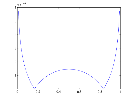
Figure 1: Error as a function of $\varepsilon$ in Experiment # 1. The superconvergent methods can be clearly seen as kinks in the error graph (corresponding to the first term in the asymptotic expansion of the error going through a zero). The methods becomes unstable as $\varepsilon\to\mathbb{Z}$. Although our analysis does not cover this case, it is clear from the graph that $\varepsilon=1/2$ continues smoothly the error graph.

Experiment #2 (Richardson extrapolation).

With the same geometric configuration, exact solution, and numerical scheme as in the superconvergent case ($\varepsilon=1/6$), we apply Richardson extrapolation to propose the potential

$$U_{h}^{\star}:={\textstyle\frac{4}{3}}U_{h/2}-{\textstyle\frac{1}{3}}U_{h},$$

as an improved approximation of the solution. The result of Proposition 12 points clearly to the existence of an asymptotic expansion of the error, very much in the style of those obtained for operator equations of zero or negative order in [2]. The numerical result shown in Table 2 corresponding maximum errors $e_{h}:=\max_{\mathbf{z}\in\mathrm{O}}|U(\mathbf{z})-U_{h}(\mathbf{z})|=\mathcal{O}(h^{3}).$

$N$	error	e.c.r
10	4.3437$E(-006)$
20	7.4235$E(-008)$	5.8707
40	5.6231$E(-009)$	3.7227
80	6.6107$E(-010)$	3.0885
160	8.1033$E(-011)$	3.0282
320	1.0052$E(-011)$	3.0110

Table 2: Errors and estimated convergence rates for Experiment #2: Richardson extrapolation applied to one of the surperconvergent methods ($\varepsilon=1/6$). Errors are computed in several external observation points. The result reported with $N=20$ uses a grid of $20$ points as $h-$grid and a refined grid of $40$ points as $h/2-$grid.

Experiment #3 (direct method).

We now apply a direct boundary integral equation method for the same exterior Neumann problem as in the previous experiments. This leads to a $2\times 2$ system with the same matrix of operators as in the previous formulation, but the adjoint double layer operator appears in the right-hand side of the system. This operator is simply discretized with midpoint formulas on each of the intervals: see [4] for a similar treatment in systems related to the single layer potential. With this formulation, the unknown is the parametrized form of the trace of the exact solution $\varphi=U\circ\mathbf{x}$ and we can thus compare $L^{\infty}$ errors (Theorems 3 and 4). We measure maximum absolute value of errors for $\varphi$ on the points $t_{j}$. The results are reported in Table 3.

$N$	boundary error	e.c.r
10	4.8555$E(-001)$
20	1.3426$E(-001)$	1.8546
40	5.4891$E(-002)$	1.2904
80	2.4641$E(-002)$	1.1555
160	1.1792$E(-002)$	1.0632
320	5.7677$E(-003)$	1.0318
640	2.8527$E(-003)$	1.0157

$N$	boundary error	e.c.r
10	2.0406$E(-001)$
20	3.5629$E(-002)$	2.5179
40	8.6392$E(-003)$	2.0441
80	2.1497$E(-003)$	2.0068
160	5.3603$E(-004)$	2.0037
320	1.3385$E(-004)$	2.0017
640	3.3444$E(-005)$	2.0008

Table 3: Errors and estimated convergence rates for Experiment #3. The leftmost table corresponds to $\varepsilon=1/3$ (order one) and the rightmost table to $\varepsilon=1/6$. The table shows errors $\|\varphi_{h}-I_{h}\varphi\|_{L^{\infty}}$.

Experiment #4 (condition numbers).

In this final experiment, we pick the matrix of the previous examples and compute its spectral condition number. We then show how a Calderón preconditioner based on premultiplying the matrix $\mathrm{W}_{ij}$ by a matrix [2, 4]

$$\mathrm{V}_{ij}=H^{(1)}_{0}(k|\mathbf{x}(t_{i})-\mathbf{x}(t_{j+\varepsilon})|)$$ (79)

reduces the condition number of the resulting system to what is basically a constant $h-$independent condition number.

N	cond VW	cond W
10	6.9548	5.7212
20	6.5994	11.7992
40	6.5349	23.7403
80	6.5196	47.5489
160	6.5159	95.1320
320	6.5150	190.2811
640	6.5148	380.5709

Table 4: Condition numbers for the matrix $\mathrm{W}$ of Experiments # 1 and # 2 and for the matrix $\mathrm{V}\mathrm{W}$, with $\mathrm{V}$ given by (79).

Appendix A Second order asymptotics

This section contains the proof of Proposition 12. Note that this result is required for the proof of $L^{\infty}$ convergence of the superconvergent methods. In order to prove Proposition 12 we have to go one term further in the different asymptotic expansions that were used in the proofs of Propositions 9 and 10.

A.1 Technical background

Lemma 11.

There exists $C$ such that for all $\varepsilon$ and $h$

$$\Big{|}\{Q_{h,\varepsilon}^{-1}\psi_{h},u\}-(\psi_{h},u)+{\textstyle\frac{h^{2}}{24}}\{Q_{h,\varepsilon}^{-1}\psi_{h},u^{\prime\prime}\}\Big{|}\leq Ch^{3}\|\psi_{h}\|_{0}\|u\|_{3}\qquad\forall\psi_{h}\in S_{h,\varepsilon},\,u\in H^{3}.$$

Proof.

It is based on the same ideas as the proof of Lemma 9, using the inequality

$$\Big{|}\int_{c-\frac{h}{2}}^{c+\frac{h}{2}}u(t)\mathrm{d}t-hu(c)-\frac{h^{3}}{24}u^{\prime\prime}(c)\Big{|}\leq Ch^{3}\int_{c-\frac{h}{2}}^{c+\frac{h}{2}}|u^{(3)}(t)|\mathrm{d}t,$$

as starting point. ∎

Proposition 13.

Let $a_{1},a_{2},a_{3}\in\mathcal{D}$ and consider an operator

$$\mathrm{V}:=\bm{a}_{1}\mathrm{H}\mathrm{D}_{-1}+\bm{a}_{2}\mathrm{H}\mathrm{D}_{-2}+\bm{a}_{3}\mathrm{H}\mathrm{D}_{-3}+\mathrm{K}_{4}\qquad\mbox{where $\mathrm{K}_{4}\in\mathcal{E}(-4)$}.$$

Let then $\mathrm{L}_{1}:=\bm{a}_{1}$, $\mathrm{L}_{2}:=\bm{a}_{1}\mathrm{D}-\bm{a}_{2}$, $\mathrm{L}_{3}:=\bm{a}_{1}\mathrm{D}^{2}-2\bm{a}_{2}\mathrm{D}+\bm{a}_{3},$ and consider the operators

$$R_{h}^{\#}u := \mathrm{V}u-\mathrm{V}Q_{h}^{-1}F_{h}u+\sum_{\ell=1}^{2}h^{\ell}\underline{C}_{\ell}(\,\cdot\,/h)\mathrm{L}_{\ell}F_{h}u,$$

$$T_{h}^{\#}u := \mathrm{V}u-\mathrm{V}Q_{h,1/2}^{-1}F_{h}u+\sum_{\ell=1}^{3}h^{\ell}\underline{C}_{\ell}(\,\cdot\,/h+1/2)\mathrm{L}_{\ell}F_{h}u.$$

Then

$$\|R_{h}^{\#}u\|_{0}+h\|R_{h}^{\#}u\|_{1} \leq Ch^{3}\|u\|_{2}\qquad\forall u\in H^{2},$$ (80)

$$\|T_{h}^{\#}u\|_{0}+h\|T_{h}^{\#}u\|_{1} \leq Ch^{4}\|u\|_{3}\qquad\forall u\in H^{3}.$$ (81)

Proof.

It is a direct consequence of [2, Proposition 16]. ∎

Proposition 14.

Let $E_{h}^{\#}u:=u-D_{h}u+\sum_{\ell=1}^{2}h^{\ell}\underline{B}_{\ell}(\,\cdot\,/h+1/2)F_{h}u^{(\ell)}.$ Then

$$\|E_{h}^{\#}u\|_{0}+h\|E_{h}^{\#}u\|_{1}\leq Ch^{3}\|u\|_{3}\qquad\forall u\in H^{3}.$$

Proof.

See [5, Proposition 1] and the proof of [2, Proposition 16]. ∎

A.2 Proof of Proposition 12

Following (5.3) and (62), we consider the decomposition of the consistency error in five terms

$$w_{h}(\psi_{h},\varphi_{h}-D_{h}\varphi)=w_{h}(\psi_{h},\varphi_{h}-\varphi)+w_{h}(\psi_{h},\varphi-D_{h}\varphi)=(T_{1}+T_{2}+T_{3})+(T_{4}+T_{5}).$$ (82)

To bound $T_{1}$ we use Lemma 11 with $u=\mathrm{D}\mathrm{V}_{1}\mathrm{D}$:

$$\Big{|}T_{1}-{\textstyle\frac{h^{2}}{24}}\{Q_{h,\varepsilon}^{-1}\psi_{h},\mathrm{D}^{3}\mathrm{V}_{1}\mathrm{D}\varphi\}\Big{|}\leq Ch^{3}\|\psi_{h}\|_{0}\|\varphi\|_{4}.$$ (83)

Proceeding as in (57) we can bound

$$|T_{2}|\leq Ch^{3}\|\psi_{h}\|_{0}\|\varphi\|_{3}.$$ (84)

To expand $T_{3}$ we use Proposition 13 applied to $\mathrm{V}_{2}$ and (50) to obtain

$$T_{3} \!\!=\!\! -h\underline{C}_{1}(\varepsilon)(Q_{h,\varepsilon}^{-1}\psi_{h},\bm{a}\varphi)-h^{2}\underline{C}_{2}(\varepsilon)(Q_{h,\varepsilon}^{-1}\psi_{h},(\bm{a}\mathrm{D}-\bm{b})\varphi)$$

$$+\underbrace{h\underline{C}_{1}(\varepsilon)(Q_{h,\varepsilon}^{-1}\psi_{h},\bm{a}(\varphi-F_{h}\varphi))}_{T_{3a}}+\underbrace{h^{2}\underline{C}_{2}(\varepsilon)(Q_{h,\varepsilon}^{-1}\psi_{h},(\bm{a}\mathrm{D}-\bm{b})(\varphi-F_{h}\varphi))}_{T_{3b}}$$

$$+\underbrace{(Q_{h,\varepsilon}^{-1}\psi_{h},R_{h}^{\#}\varphi)}_{T_{3c}}.$$

We now use Lemma 9(b) and (50) to bound $|T_{3a}|+|T_{3b}|\leq Ch^{3}\|\psi_{h}\|_{0}\|\varphi\|_{2},$ as well as Lemma 9(b) and (80) to bound $|T_{3c}|\leq Ch^{3}\|\psi_{h}\|_{0}\|\varphi\|_{2}.$ Therefore

$$|T_{3}+h\underline{C}_{1}(\varepsilon)(Q_{h,\varepsilon}^{-1}\psi_{h},\bm{a}\varphi)+h^{2}\underline{C}_{2}(\varepsilon)(Q_{h,\varepsilon}^{-1}\psi_{h},(\bm{a}\mathrm{D}-\bm{b})\varphi)|\leq Ch^{3}\|\psi_{h}\|_{0}\|\varphi\|_{2}.$$ (85)

To expand $T_{4}$ we use Proposition 13 applied to $\mathrm{V}_{1}$. Note that $\mathrm{L}_{1}=\alpha\mathrm{I}$, $\mathrm{L}_{2}=\alpha\mathrm{D}-\bm{c}$ and $\mathrm{L}_{3}\in\mathcal{E}(2)$. Because of (63), we can write

$$T_{4} = \sum_{\ell=1}^{2}h^{\ell}\underline{C}_{\ell}(\varepsilon)(Q_{h,\varepsilon}^{-1}\psi_{h},\mathrm{D}\mathrm{L}_{\ell}\mathrm{D}\varphi)$$

$$+\sum_{\ell=1}^{2}\underline{C}_{\ell}(\varepsilon)\Big{(}\underbrace{h^{\ell}(\psi_{h}-Q_{h,\varepsilon}^{-1}\psi_{h},\mathrm{D}\mathrm{L}_{\ell}\mathrm{D}\varphi)}_{T_{4a}^{\ell}}+\underbrace{h^{\ell}(\psi_{h}^{\prime},\mathrm{L}_{\ell}(\varphi^{\prime}-F_{h}\varphi^{\prime}))}_{T_{4b}^{\ell}}\Big{)}$$

$$-\underbrace{h^{3}\underline{C}_{3}(\varepsilon)(\psi_{h}^{\prime},\mathrm{L}_{3}F_{h}\varphi^{\prime})}_{T_{4c}}+\underbrace{(\psi_{h}^{\prime},T_{h}^{\#}\varphi^{\prime})}_{T_{4d}}.$$

Using Lemma 9(a) and (48) we can bound

$$|T_{4a}^{1}|+|T_{4a}^{2}|\leq Ch^{3}\|\psi_{h}\|_{0}\left(\|\mathrm{D}\mathrm{L}_{1}\mathrm{D}\varphi\|_{2}+\|\mathrm{D}\mathrm{L}_{2}\mathrm{D}\varphi\|_{1}\right)\leq C^{\prime}h^{3}\|\psi_{h}\|_{0}\|\varphi\|_{4}.$$

By (50) (and using the commutation $\mathrm{D}F_{h}=F_{h}\mathrm{D}$ to simplify some expressions) we next bound

$$|T_{4b}^{1}|+|T_{4b}^{2}| \leq \|\psi_{h}\|_{0}\Big{(}h\|\mathrm{D}\mathrm{L}_{1}\mathrm{D}(\varphi-F_{h}\varphi)\|_{0}+h^{2}\|\mathrm{D}\mathrm{L}_{2}\mathrm{D}(\varphi-F_{h}\varphi)\|_{0}\Big{)}$$

$$\leq C\|\psi_{h}\|_{0}\Big{(}h\|\varphi-F_{h}\varphi\|_{2}+h^{2}\|\varphi-F_{h}\varphi\|_{3}\Big{)}\leq C^{\prime}h^{3}\|\psi_{h}\|_{0}\|\varphi\|_{4}.$$

Similarly

$$|T_{4c}|\leq h^{3}|\underline{C}_{3}(\varepsilon)|\|\psi_{h}\|_{0}\|\mathrm{D}\mathrm{L}_{3}\mathrm{D}F_{h}\varphi\|_{0}\leq C\,h^{3}\|\psi_{h}\|_{0}\|\varphi\|_{4}.$$

Finally, by (81)

$$|T_{4d}|\leq\|\psi_{h}\|_{0}\|\mathrm{D}T_{h}^{\#}\varphi^{\prime}\|_{0}\leq Ch^{3}\|\psi_{h}\|_{0}\|\varphi\|_{4}.$$

Collecting all these bounds we have just proved that

$$\Big{|}T_{4}-\sum_{\ell=1}^{2}h^{\ell}\underline{C}_{\ell}(\varepsilon)(Q_{h,\varepsilon}^{-1}\psi_{h},\mathrm{D}\mathrm{L}_{\ell}\mathrm{D}\varphi)\Big{|}\leq Ch^{3}\|\psi_{h}\|_{0}\|\varphi\|_{4}.$$ (86)

We are only left to deal with $T_{5}$. Using Proposition 14, the argument in (69), and the fact that $\underline{B}_{2}(1/2)=-1/24$, we can write

$$Q_{h}^{-1}(\varphi-D_{h}\varphi) = -h\underline{B}_{1}(1/2)Q_{h}^{-1}F_{h}\varphi^{\prime}-h^{2}\underline{B}_{2}(1/2)Q_{h}^{-1}F_{h}\varphi^{\prime\prime}+Q_{h}^{-1}E_{h}^{\#}\varphi$$

$$= \frac{h^{2}}{24}Q_{h}^{-1}F_{h}\varphi^{\prime\prime}+Q_{h}^{-1}E_{h}^{\#}\varphi.$$

Therefore,

$$T_{5} = \frac{h^{2}}{24}\{Q_{h,\varepsilon}^{-1}\psi_{h},\mathrm{V}_{2}Q_{h}^{-1}F_{h}\varphi^{\prime\prime}\}+\{Q_{h,\varepsilon}^{-1}\psi_{h},\mathrm{V}_{2}Q_{h}^{-1}E_{h}^{\#}\varphi\}$$

$$= \frac{h^{2}}{24}(Q_{h,\varepsilon}^{-1}\psi_{h},\mathrm{V}_{2}\varphi^{\prime\prime})$$

$$+\underbrace{\frac{h^{3}}{24}\underline{C}_{1}(\varepsilon)(Q_{h,\varepsilon}^{-1}\psi_{h},\bm{a}F_{h}\varphi^{\prime\prime})}_{T_{5a}}-\underbrace{\frac{h^{2}}{24}(Q_{h,\varepsilon}^{-1}\psi_{h},R_{h}\varphi^{\prime\prime})}_{T_{5b}}+\underbrace{\{Q_{h,\varepsilon}^{-1}\psi_{h},\mathrm{V}_{2}Q_{h}^{-1}E_{h}^{\#}\varphi\}}_{T_{5c}},$$

where we have applied Proposition 7. By Lemma 9(b) and (53) we can bound $|T_{5a}|+|T_{5b}|\leq Ch^{3}\|\psi_{h}\|_{0}\|\varphi\|_{3},$ while by Lemma 10 and Proposition 14, we can bound $|T_{5c}|\leq Ch^{3}\|\psi_{h}\|_{0}\|\varphi\|_{3}.$ Therefore

$$\Big{|}T_{5}-\frac{h^{2}}{24}(Q_{h,\varepsilon}^{-1}\psi_{h},\mathrm{V}_{2}\varphi^{\prime\prime})\Big{|}\leq Ch^{3}\|\psi_{h}\|_{0}\|\varphi\|_{3}.$$ (87)

The result is the combination of (82)-(87).

References

- [1] D. N. Arnold. A spline-trigonometric Galerkin method and an exponentially convergent boundary integral method. Math. Comp., 41(164):383–397, 1983.
- [2] R. Celorrio, V. Domínguez, and F. J. Sayas. Periodic Dirac delta distributions in the boundary element method. Adv. Comput. Math., 17(3):211–236, 2002.
- [3] V. Domínguez, S. L. Lu, and F.-J. Sayas. Fully discrete Calderón Calculus for the two dimensional Helmholtz equation. In preparation.
- [4] V. Domínguez, M.-L. Rapún, and F.-J. Sayas. Dirac delta methods for Helmholtz transmission problems. Adv. Comput. Math., 28(2):119–139, 2008.
- [5] V. Domínguez and F.-J. Sayas. Full asymptotics of spline Petrov-Galerkin methods for some periodic pseudodifferential equations. Adv. Comput. Math., 14(1):75–101, 2001.
- [6] V. Domínguez and F.-J. Sayas. Local expansions of periodic spline interpolation with some applications. Math. Nachr., 227:43–62, 2001.
- [7] G. C. Hsiao and W. L. Wendland. Boundary integral equations, volume 164 of Applied Mathematical Sciences. Springer-Verlag, Berlin, 2008.
- [8] W. McLean. Strongly elliptic systems and boundary integral equations. Cambridge University Press, Cambridge, 2000.
- [9] J. Saranen and L. Schroderus. Quadrature methods for strongly elliptic equations of negative order on smooth closed curves. SIAM J. Numer. Anal., 30(6):1769–1795, 1993.
- [10] J. Saranen and I. H. Sloan. Quadrature methods for logarithmic-kernel integral equations on closed curves. IMA J. Numer. Anal., 12(2):167–187, 1992.
- [11] J. Saranen and G. Vainikko. Periodic Integral and Pseudodifferential Equations with Numerical Approximation. Springer Monographs in Mathematics. Springer-Verlag, Berlin, 2002.
- [12] S. A. Sauter and C. Schwab. Boundary element methods, volume 39 of Springer Series in Computational Mathematics. Springer-Verlag, Berlin, 2011.
- [13] I. H. Sloan and B. J. Burn. An unconventional quadrature method for logarithmic-kernel integral equations on closed curves. J. Integral Equations Appl., 4(1):117–151, 1992.