A Direct Approach to Multi-class Boosting and Extensions

Abstract

Boosting methods combine a set of moderately accurate weak learners to form a highly accurate predictor. Despite the practical importance of multi-class boosting, it has received far less attention than its binary counterpart. In this work, we propose a fully-corrective multi-class boosting formulation which directly solves the multi-class problem without dividing it into multiple binary classification problems. In contrast, most previous multi-class boosting algorithms decompose a multi-boost problem into multiple binary boosting problems. By explicitly deriving the Lagrange dual of the primal optimization problem, we are able to construct a column generation-based fully-corrective approach to boosting which directly optimizes multi-class classification performance. The new approach not only updates all weak learners’ coefficients at every iteration, but does so in a manner flexible enough to accommodate various loss functions and regularizations. For example, it enables us to introduce structural sparsity through mixed-norm regularization to promote group sparsity and feature sharing. Boosting with shared features is particularly beneficial in complex prediction problems where features can be expensive to compute. Our experiments on various data sets demonstrate that our direct multi-class boosting generalizes as well as, or better than, a range of competing multi-class boosting methods. The end result is a highly effective and compact ensemble classifier which can be trained in a distributed fashion.

Keywords: multi-class boosting, Lagrange duality, column generation, convex optimization, distributed optimization, alternating direction methods

1 Introduction

A significant proportion of the most important practical classification problems inherently involve making a selection between a large number of classes. Such problems demand effective and efficient multi-class classification techniques. Unlike binary classification, which has been well researched, multi-class classification has received relatively little attention due to the inherent complexity of the problem. Some important steps have been (see Wu et al. (2004); Crammer and Singer (2001); Guruswami and Sahai (1999) for instance), but the primary approach thus far has exploited large numbers of independent binary classifiers. An example of this approach is the extension of a binary classification algorithm to the multi-class case by considering the problem as a set of one-vs-all binary classification problems.

Boosting has recently attracted much research interest in many scientific fields due to its huge success in classification and regression tasks, especially in the first real-time face detection application (Viola and Jones, 2004). Both theoretical and empirical results show that boosting methods have competitive generalization performance compared with many existing classifiers in the literature. To explain why boosting works, Schapire et al. (1998) introduced an appropriate margin theory, which was inspired by the margin theory in support vector machines, and concluded that boosting is also an effective classifier which maximizes the minimum margin over the training data. Extending this idea, LPBoost (Demiriz et al., 2002) seeks to maximize the relaxed minimum margin (soft margin) using hinge loss. The proposed boosting algorithm is fully corrective in the sense that all the coefficients of learned weak classifiers are updated at each iteration. Such fully-corrective boosting algorithms typically require fewer iterations to achieve convergence.

Despite the significant attention that boosting-based binary classification methods have attracted, multi-class boosting has been much less well studied. As with multi-class classification in general, the most natural strategy for multi-class boosting is to partition the problem into a set of independent binary classification problems. In this scenario each binary classifier is charged with distinguishing a subset of the classes against all others. Methods such as one-vs-all, all-vs-all and output code-based methods belong to this category. Although such partitioning strategies greatly simplify the problem, they inevitably impact upon the final solution. In many cases the partitioning strategy changes the cost function to be optimized, and thus delivers a sub-optimal solution. The all-vs-all approach, a.k.a. one-vs-one, however, has been shown to achieve excellent classification accuracy. In this approach $k(k-1)/2$ two-way pairwise classifiers are trained, with $k$ the number of classes. The computation of both training and testing can be prohibitively expensive even when $k$ is of medium size. More importantly, however, almost all of these strategies do not directly optimize the multi-class decision function that they seek to exploit.

In this work, we proffer a direct approach to fully-corrective multi-class boosting. In order to achieve this result, we generalize the concept of the separating hyperplane and margin in binary boosting to multi-class problems. This allows the development of a single, fully-corrective, multi-class boosting classifier which directly optimizes multi-class classification performance. Similar ideas have been used in multi-class support vector machines (Crammer and Singer, 2001; Weston and Watkins, 1999; Elisseeff and Weston, 2001). To our knowledge, it has not been employed to design fully-corrective multi-class boosting. As shown in (Shen and Li, 2010) fully-corrective boosting in general leads to more compact models. Here for the first time, we develop fully-corrective multi-class boosting.

In deriving out direct formulation we also generalize the fully-corrective $\ell_{1}$ regularized boosting algorithms to arbitrary mixed-norm regularization terms. Mixed-norm regularization, also known as group sparsity, has been used when there exists a structure that separates the model into disjoint groups of parameters. For $\ell_{1,2}$-norm regularized boosting, for example, each such group of parameters is subject to a common $\ell_{2}$-norm regularizer. The key intuition behind structural sparsity is that informative features are commonly shared between multiple classes. For example, traffic warning signs have a common triangular shape with various symbols inside. These basic shared features should be used to help differentiate warning signs from other traffic signs while the symbols inside can be used to differentiate different warning signs. In this work, we aim to enable the selection of a common subset of features which are informative in identifying a wide range of classes.

The key idea behind our column generation-based boosting approach is that, given an example ${\boldsymbol{x}}$, with true label $y$, the output of the decision function for the correct label must be larger than the output of the decision function for all incorrect labels,

$$F_{y}(\boldsymbol{x})>F_{r}(\boldsymbol{x}),\,\,\forall r\neq y.$$

We then formulate a convex optimization problem, which maximizes $F_{y}(\boldsymbol{x})-F_{r}(\boldsymbol{x})$ subject to the selected regularization term. This leads to a constrained semi-infinite convex optimization problem, which may have infinitely many variables. In order to design a boosting algorithm, we explicitly derive the Lagrange dual of this problem and apply an iterative convex optimization technique known as column generation. When the hinge loss is used, our formulation can be viewed as a direct extension of LPBoost (Demiriz et al., 2002) to the multi-class case. We also discuss the use of the exponential and logistic loss functions. In theory, any convex loss function can be employed, as in the binary classification case. Note that the AnyBoost framework of Mason et al. (2000) can not be adopted here since AnyBoost cannot cope with multiple constraints. In summary, our main contributions are as follows.

• We propose the first direct approach to fully-corrective multi-class boosting based on the generalization of the conventional “margin” in binary classification.

• Within this direct, fully corrective boosting framework, we design new boosting methods that promote feature sharing across classes by enforcing group sparsity regularization (referred to as MultiBoost${}^{\,\rm group}$). We empirically show that by enforcing group sparsity, the proposed multi-class boosting converges faster while achieving better or comparable generalization performance. The fact that the algorithm converges fast means that fewer features are required for a given classification accuracy and there is a significant improvement in run-time performance. Our derivation for designing multi-class boosting methods is applicable to arbitrary convex loss functions with general $\ell_{1,p}$ $(p\geq 1)$ mixed-norms. To our knowledge, this is the first fully-corrective multi-class boosting approach that promotes feature sharing using group sparsity regularization. Moreover, we propose the use of the alternating direction method of multipliers (ADMM) (Boyd et al., 2011) to efficiently solve the involved optimization problems, which is much faster than using standard interior-point solvers.

• Further, a new family of multi-class boosting algorithms based on a simplified formulation is proposed in order to further reduce training times. This new formulation not only enables us to share features and encourages structural sparsity in the learning procedure of multi-class boosting, but also allows us to take advantage of parallelism in ADMM to speed up the training time by a factor proportional to the number of classes. The training time required is thus similar to that required to train multiple independent binary classifiers in parallel. The proposed formulation converges significantly faster, while still enforcing group sparsity.

Since multi-class classification can be seen as an instance of structured learning problems of Tsochantaridis et al. (2005), the proposed formulation may also be applicable to other structured prediction problems.

We briefly review most relevant work on multi-class boosting before we present our algorithms.

1.1 Related work

AdaBoost, proposed in (Freund and Schapire, 1997), was the first practical binary boosting algorithm. One of the limitations of binary AdaBoost is that each weak classifier’s accuracy must be higher than $0.5$. That is, a weak classifier must exhibit classification capability superior to that of random guessing. AdaBoost.M1, directly extended AdaBoost to multi-class classification using multi-class weak classifiers. Multi-class weak classifiers, such as decision trees for example, represent a restricted set of weak classifiers able to give predictions on all $k$ possible labels at each call. The fact that only multi-class weak classifiers can be used represents a significant restriction, as multi-class weak classifiers are complicated and require time-consuming training when compared with their simple binary counterparts. The higher complexity of the assembled classifier also implies a higher risk of over-fitting the training data. In addition, the requirement that a weak classifier’s weighted error must be better than $0.5$ can be hard to achieve for problems with many classes. Note that, for a problem with $k$ classes, random guessing can only guarantee an accuracy of $1/k$.

The SAMME algorithm of Zhu et al. (2009), addressed this last issue, and requires only that the multi-class weak classifiers achieve an error rate better than uniform random guessing for multiple labels ($1/k$ for $k$ labels). When $k=2$, SAMME reduces to the standard AdaBoost, but is still subject to all of the other limitations associated with the use of multi-class weak classifiers.

To alleviate these difficulties one solution is to decompose a multi-class boosting problem into a set of binary classification problems. To this end strategies such as “one-vs-all” and “one-vs-one” have been developed. Such approaches can be viewed as special cases of error-correcting output coding (ECOC) (Dietterich and Bakiri, 1995; Crammer and Singer, 2002). By introducing a coding matrix, AdaBoost.MO (Schapire and Singer, 1999) is a typical example of ECOC based multi-class boosting. In this approach a set of binary classifiers is used, with each trained so as to recognise a subset of the classes. By comparison of the responses of all of the binary classifiers multi-class classification is achieved. Algorithms in this category include AdaBoost.MO (Schapire and Singer, 1999), AdaBoost.OC and AdaBoost.ECC (Guruswami and Sahai, 1999). AdaBoost.OC can be seen as a variant of AdaBoost.MO which also combines boosting and ECOC. However, unlike AdaBoost.MO, AdaBoost.OC uses a collection of randomly generated codewords. For more details see (Schapire, 1997).

The attraction of transforming a multi-class classification problem into a set of binary classification problems is that each of the weak classifiers need only be a simple binary classifier. This approach has its limitations, however, including the fact that the required optimisation problem is typically compromised by the partition, and that it becomes increasingly difficult to ensure that each binary classifier sees a representative sample of the data as the number of classes increases. An additional limitation of all partitioning algorithms we have discussed is that they are incapable of effectively exploiting the inevitable similarity between classes, and thus to efficiently share features between classifiers. Since binary classifiers are trained independently, the resulting strong classifier can be highly unbalanced and often dependent on an excessive number of features/weak classifiers.

Several approaches have been developed which aim to enable feature-sharing within multi-class boosting. JointBoost, proposed by Torralba et al. (2007), finds common features that can be shared across classes using heuristics. Weak learners are then trained jointly using standard boosting. In order to reduce the number of binary classifiers which need to be trained for multi-class problems, the authors proposed an approximate search procedure based on greedy forward selection. The drawback of greedy approach, however, is that it is short-sighted and cannot recover if an error is made. The fact that the weak learner selected at each boosting iteration cannot be guaranteed to be globally optimal means that the final ensemble is highly likely to be sub-optimal. Zhang et al. proposed training multi-class boosting with sharable information patterns (Zhang et al., 2009). As a pre-processing step, they generate sharable patterns using data mining techniques and then train a multi-class boosting-based classifier using these patterns. The process of identifying sharable features and the training procedure are thus de-coupled, and therefore unlikely to reach the optimal solution. In comparison to JointBoost and Zhang et al.’s work, the method we propose selects weak learners systematically on the basis of structural sparsity during the training process and thus, at least asymptotically, will reach the globally optimal solution.

A related approach, termed GradBoost (Duchi and Singer, 2009), also exploits a mixed-norm in order to achieve group sparsity, but does not directly optimize the boosting objective function. Instead, the algorithm updates a block of variables for optimizing a quadratic surrogate function in a fashion similar to gradient-based coordinate descent. It is not clear how well the surrogate approximates the original objective function, and no proof is given. Since the mixed-norm regularization term is not directly optimized either, group sparsity is achieved heuristically by a combination of forward selection and backward elimination. Our work fundamentally differs from (Duchi and Singer, 2009) in that we directly optimize the group sparsity regularized objective by following the column generation based boosting (Shen and Li, 2010) without deferring to heuristics.

Our work here can also be seen as an extension of the general binary fully-corrective boosting framework of Shen and Li (2010) to the multi-class case. As in (Shen and Li, 2010), we design a feature-sharing boosting method using a direct formulation, but for multi-class problems and using a more sophisticated group sparsity regularization. Note that the general boosting framework of Shen and Li (2010) is not directly applicable in our problem setting.

1.2 Notation

A bold lowercase letter ($\boldsymbol{u}$) denotes a column vector, and an uppercase letter ($U$) a matrix. $\operatorname{\bf Tr}(U)$ represents the trace of a symmetric matrix. An element-wise inequality between two vectors or matrices such as ${\boldsymbol{u}}\geq{\boldsymbol{v}}$ implies that $u_{i}\geq v_{i}$ for all $i$.

Let $({\boldsymbol{x}}_{i};y_{i})\in\mathbb{R}^{d}\times\{1,\ldots,k\},i=1\ldots m$, be a set of $m$ multi-class training examples, where $k$ denotes the number of classes. We denote by ${\cal H}$ a set of weak classifiers (or dictionary); note that the size of ${\cal H}$ can be infinite. Each $h_{j}(\cdot)\in{\cal H},j=1\dots n$, is a function that maps an input ${\boldsymbol{x}}$ to $\{-1,+1\}$. Although our discussion applies equally in the general case where $h(\cdot)$ make take any real value, we use binary weak classifiers in this work. The matrix $H\in\mathbb{R}^{m\times n}$ captures the weak classifiers’ responses to the whole of the training data; that is $H_{ij}=h_{j}({\boldsymbol{x}}_{i})$. Each column $H_{:j}$ thus represents the output of the weak classifier $h_{j}(\cdot)$ when applied to the entire training set and each row $H_{i:}$ the responses of all of the weak classifiers to the $i$th training datum ${\boldsymbol{x}}_{i}$.

Boosting algorithms learn a strong classifier of the form $F({\boldsymbol{x}})=\sum_{j=1}^{n}w_{j}h_{j}({\boldsymbol{x}})$ which is parameterized by a vector ${\boldsymbol{w}}\in\mathbb{R}^{n}$. In our formulation of the problem we need to learn a classifier for each class. So for class $r$ (where $r=1,\ldots,k$), the learned strong classifier is $F_{r}({\boldsymbol{x}})=\sum_{j=1}^{n}w_{r,j}h_{j}({\boldsymbol{x}})$ and has parameter vector ${\boldsymbol{w}}_{r}$. We define $W=[{\boldsymbol{w}}_{1},{\boldsymbol{w}}_{2},\ldots,{\boldsymbol{w}}_{k}]\in\mathbb{R}^{n\times k}$ and let $\left\|W\right\|_{\mathrm{1}}=\sum_{ij}|W_{ij}|$ represent the $\ell_{1}$ norm. The $\ell_{1,2}$ norm of a matrix is defined as $\|W\|_{1,2}=\sum_{j}\|W_{j:}\|_{2}$ with $\|\cdot\|_{2}$ being the $\ell_{2}$ norm. The $\ell_{1,\infty}$ norm of $W$ is $\|W\|_{1,\infty}=\sum_{j}\max(W_{j:})$.

Here we assume that the weak classifier dictionary for each class is the same. The final strong classifier is a weighted average of multiple weak classifiers, and the estimated classification for a test datum ${\boldsymbol{x}}$ is $F({\boldsymbol{x}})=\mathop{\mathrm{argmax}}\limits_{r=1,\dots k}\,\sum_{j=1}^{n}w_{r,j}h_{j}({\boldsymbol{x}}).$

The remaining content is structured as follows. Section 2 presents the main algorithm of our work. In particular, we beginning by deriving our algorithm with $\ell_{1}$ penalty for the piece-wise linear hinge loss and exponential loss functions. Then we discuss group sparsity and derive our algorithm with the new structural sparsity for both hinge loss and logistic loss. We present our experimental results in Section 3.1 and conclude in Section 4.

2 A direct formulation for multi-class boosting

In binary classification, the margin is defined as $yF(\boldsymbol{x})$ with $y\in\{-1,+1\}$. In the framework of maximum margin learning, one tries to maximize the margin $yF(\boldsymbol{x})$ as much as possible. A large margin implies the learned classifier confidently classifies the corresponding training example. We show how this idea can be generalized to multi-class problems in this section.

2.1 MultiBoost with $\ell_{1}$-norm regularization (MultiBoost${}^{\,\ell_{1}}$)

The hinge loss

Let us consider the hinge loss case, which is piecewise linear and therefore makes it easy to derive our formulation. As we will show, both the primal and dual problems are linear programs (LPs), which can be globally solved in polynomial time. The basic idea is to learn classifiers by pairwise comparison. For a training example $({\boldsymbol{x}},y)$, if we have a perfect classification rule, then the following holds

$$F_{y}({\boldsymbol{x}})>F_{r}({\boldsymbol{x}}),\text{ for any }r\neq y.$$

In the large margin framework with the hinge loss, ideally

$$F_{y}({\boldsymbol{x}})\geq 1+F_{r}({\boldsymbol{x}}),\text{ for any }r\neq y,$$ (1)

should be satisfied. This means that the correct label is supposed to have a classification confidence that is larger by at least a unit than any of the confidences for the other predictions. This extension of “margin” to the multi-class case has been introduced in support vector machines (Weston and Watkins, 1999; Elisseeff and Weston, 2001). As pointed out in Weston and Watkins (1999), to formulate multi-class problems as a pairwise ranking problem in a single optimization can be more powerful than to solve a bunch of one-vs-all binary classifications. The argument is that we may generate a multi-class data set that can be classified perfectly, but for which the training data cannot be separated with no error by one-vs-all. Recent work in (Daniely et al., 2012) theoretically proved that the direct approach to multi-class classification essentially contains the hypothesis classes of one-vs-all. Also because the estimation errors of these two methods are roughly the same, the direct approach dominates one-vs-all in terms of achievable classification performance.

By introducing the indication operator $\delta_{s,t}$ such that $\delta_{s,t}=1$ if $s=t$ and $\delta_{s,t}=0$ otherwise, the above equation can be simplified as

$$\delta_{r,y}+F_{y}({\boldsymbol{x}})\geq 1+F_{r}({\boldsymbol{x}}),\forall r=1,2,\ldots,k.$$ (2)

We generalize this idea to the entire training set and introduce slack variables ${\boldsymbol{\xi}}$ to enable soft-margin. The primal problem that we want to optimize can then be written as

$$\min_{W,{\boldsymbol{\xi}}}\; \sum_{i=1}^{m}\xi_{i}+\nu\left\|W\right\|_{\mathrm{1}}$$

$$\;\mathop{\mathrm{s.t.\!\!:}}\nolimits\; \delta_{r,{y_{i}}}+H_{i:}{\boldsymbol{w}}_{y_{i}}\geq 1+H_{i:}{\boldsymbol{w}}_{r}-\xi_{i},\forall i,r,\;W\geq 0.$$ (3)

Here $\nu>0$ is the regularization parameter. ${\boldsymbol{\xi}}\geq 0$ always holds. If for a particular ${\boldsymbol{x}}_{i}$, $\xi_{i}$ is negative, then one of the constraint in (2.1) that corresponds to the case $r=y_{i}$ will be violated. In other words, the constraint corresponding to the case $r=y_{i}$ ensures the non-negativeness of $\boldsymbol{\xi}$. Note that we have one slack variable for each training example. It is also possible to assign a slack variable to each constraint in (2.1). We derive its Lagrange dual, similar to case of LPBoost (Demiriz et al., 2002). The Lagrangian of problem (2.1) can be written as

$$L=\sum_{i}\xi_{i}+\nu\sum_{j,r}W_{jr}-\sum_{i,r}U_{ir}\cdot\bigl{(}\delta_{r,y_{i}}+H_{i:}{\boldsymbol{w}}_{y_{i}}-1-H_{i:}{\boldsymbol{w}}_{r}+\xi_{i}\bigr{)}-\operatorname{\bf Tr}(V^{\!\top}W),$$

with $U\geq 0$, $V\geq 0$. At optimum, the first derivative of the Lagrangian w.r.t. the primal variables must vanish,

$$\frac{\partial L}{\partial\xi_{i}}=0\longrightarrow\sum_{r}U_{ir}=1,\forall i.$$ (4)

Also,

$$\frac{\partial L}{\partial{\boldsymbol{w}}_{r}} ={\boldsymbol{0}}\longrightarrow\nu 1^{\!\top}+\sum_{r}U_{ir}H_{i:}-\sum_{i,r=y_{i}}\underbrace{\Bigl{(}\sum_{l}U_{il}\Bigr{)}}_{=1,\text{ due to }\eqref{EQCVPR11:A1}}H_{i:}=V_{r:},$$ (5)

which leads to $\sum_{i}U_{ir}H_{i:}-\sum_{i}\delta_{r,y_{i}}H_{i:}\geq-\nu{\boldsymbol{1}}^{\!\top},\forall r.$ So the Lagrange dual can be written as:

$$\min_{U}\; \sum_{r=1}^{k}\sum_{i=1}^{m}\delta_{r,y_{i}}U_{ir}$$

$$\;\mathop{\mathrm{s.t.\!\!:}}\nolimits\; \sum_{i}\left(\delta_{r,y_{i}}-U_{ir}\right)H_{i:}\leq\nu{\boldsymbol{1}}^{\!\top},\forall r,\sum_{r}U_{ir}=1,\forall i;\;U\geq 0.$$ (6)

Each row of the matrix $U$ is normalized. The first set of constraints can be infinitely many:

$$\sum_{i}\left(\delta_{r,y_{i}}-U_{ir}\right)h({\boldsymbol{x}}_{i})\leq\nu,\forall r,\text{ and }\forall h(\cdot)\in{\mathcal{H}}.$$ (7)

We can now use column generation to solve the problem, similar to the LPBoost (Demiriz et al., 2002). The subproblem for generating weak classifiers is

$$h^{*}(\cdot)=\mathop{\mathrm{argmax}}\limits_{h(\cdot)\in\mathcal{H},r}\sum_{i=1}^{m}\left(\delta_{r,y_{i}}-U_{ir}\right)h({\boldsymbol{x}}_{i}).$$ (8)

The matrix $U\in\mathbb{R}^{m\times k}$ plays the role of measuring importance of a training example. The following algorithm can be used to implement our hinge loss based MultiBoost${}^{\,\ell_{1}}$.

Algorithm 1 MultiBoost${}^{\,\ell_{1}}$ with the hinge loss.

8

8

8

8

8

8

8

8

The exponential loss

Now let us consider the exponential loss in the section. In the case of the exponential loss, We may write the primal optimization problem as

$$\min_{W}\; \sum_{i=1}^{m}\sum_{r=1}^{k}\exp\left[-\bigl{(}H_{i:}{\boldsymbol{w}}_{y_{i}}-H_{i:}{\boldsymbol{w}}_{r}\bigr{)}\right]+\nu^{\prime}\left\|W\right\|_{\mathrm{1}},\;\mathop{\mathrm{s.t.\!\!:}}\nolimits\;W\geq 0.$$ (9)

We define a set of margins associated with a training example as

$$\rho_{i,r}=H_{i:}{\boldsymbol{w}}_{y_{i}}-H_{i:}{\boldsymbol{w}}_{r},\;r=1,\dots,k.$$ (10)

Clearly only when $\rho_{i,r}\geq 0$, will the training example ${\boldsymbol{x}}_{i}$ be correctly classified. We consider the logarithmic version of the original cost function, which does not change the problem because $\log(\cdot)$ is strictly monotonically increasing. So we write (9) into

$$\min_{W,\boldsymbol{\rho}}\;\log\Bigl{(}\sum_{i=1}^{m}\sum_{r=1}^{k}\exp\left[-\rho_{i,r}\right]\Bigr{)}+\nu\left\|W\right\|_{\mathrm{1}}\;\mathop{\mathrm{s.t.\!\!:}}\nolimits\;\;\rho_{i,r}=H_{i:}{\boldsymbol{w}}_{y_{i}}-H_{i:}{\boldsymbol{w}}_{r},\forall i,\forall r,\;W\geq 0.$$ (11)

The dual problem can be easily derived:

$$\min_{U}\; \sum_{r=1}^{k}\sum_{i=1}^{m}U_{ir}\log U_{ir}$$

$$\;\mathop{\mathrm{s.t.\!\!:}}\nolimits\; \sum_{i}\left[\delta_{r,y_{i}}\bigl{(}{\textstyle\sum_{l=1}^{k}}U_{il}\bigr{)}-U_{ir}\right]H_{i:}\leq\nu{\boldsymbol{1}}^{\!\top},\forall r;\;\sum_{i,r}U_{ir}=1,U\geq 0.$$ (12)

We can see that the dual problem is a Shanon entropy maximization problem. The objective function of the dual encourages the weights $U$ to be uniform. The KKT condition gives the relationship between the optimal primal and dual variables:

$$U_{ir}^{\star}=\frac{\exp(-\rho_{i,r}^{\star})}{\sum_{i,r}\exp(-\rho_{i,r}^{\star})},\ \forall i,r.$$ (13)

Different from the case of the hinge loss, here $U$ is normalized as an entire matrix. Also we can solve the primal problem using simple (Quasi-)Newton, which is much faster than to solve the dual problem using convex optimization solvers. Note that the scale of the primal problem is usually smaller than the dual problem. After obtaining the primal variable, we can use the KKT condition to get the dual variable. The subproblem that we need to solve for generating weak classifiers also slightly differs from (8):

$$h^{*}(\cdot)=\mathop{\mathrm{argmax}}\limits_{h(\cdot)\in\mathcal{H},r}\sum_{i=1}^{m}\Bigl{(}\delta_{r,y_{i}}\bigl{(}{\textstyle\sum_{l=1}^{k}}U_{il}\bigr{)}-U_{ir}\Bigr{)}h({\boldsymbol{x}}_{i}).$$ (14)

General convex loss

We generalize the presented idea to any smooth convex loss functions in this section. Suppose ${\Theta}(\cdot)$ is a smooth convex function defined in $\mathbb{R}$. For classification problems, ${\Theta}(\cdot)$ is usually a convex surrogate of the non-convex zero-one loss. As in the exponential loss case, we introduce a set auxiliary variables that define the margin as the pairwise difference of prediction scores. This auxiliary variable is the key to lead to the important Lagrange dual, on which the fully-corrective boosting algorithms rely.

The optimization problem can be formulated as

$$\min_{W,\boldsymbol{\rho}}\;\sum_{i=1}^{m}\sum_{r=1}^{k}{\Theta}(-\rho_{i,r})+\nu\left\|W\right\|_{\mathrm{1}}\;\mathop{\mathrm{s.t.\!\!:}}\nolimits\; \eqref{EQCVPR11:margin},{\rm and}\;\,W\geq 0.$$ (15)

The Lagrangian is

$$L=\sum_{i,r}{\Theta}(-\rho_{i,r})-\operatorname{\bf Tr}(V^{\!\top}W)+\sum_{i,r}U_{ir}(H_{i:}{\boldsymbol{w}}_{y_{i}}-H_{i:}{\boldsymbol{w}}_{r})-\sum_{i,r}U_{ir}\rho_{i,r}+\nu\sum_{j,r}W_{jr}.$$

We can again write its Lagrange dual as

$$\min_{U}\;\sum_{r=1}^{k}\sum_{i=1}^{m}{\Theta}^{*}(-U_{ir})\;\mathop{\mathrm{s.t.\!\!:}}\nolimits\;\sum_{i}\left[\delta_{r,y_{i}}\bigl{(}{\textstyle\sum_{l=1}^{k}}U_{il}\bigr{)}-U_{ir}\right]H_{i:}\leq\nu{\boldsymbol{1}}^{\!\top},\forall r,$$ (16)

where ${\Theta}^{*}(\cdot)$ is the Fenchel dual function of ${\Theta}(\cdot)$ (Boyd and Vandenberghe, 2004). Note that ${\Theta}^{*}(\cdot)$ is always convex even if the original loss function ${\Theta}(\cdot)$ is non-convex. The difference is that the duality gap is not zero when ${\Theta}(\cdot)$ is non-convex. The KKT condition establishes the connection between the dual variable $U$ and the primal variable at optimality:

$$U_{ir}^{\star}=-\nabla{\Theta}(\rho_{i,r}^{\star}).$$ (17)

So we can actually solve the primal problem and then recover the dual solution from the primal. From (17), we know that the weight $U$ is typically non-negative for classification problems because the classification loss function ${\Theta}(\cdot)$ is monotonically decreasing and its gradient is non-positive.

In the next section we formulate the multi-class boosting algorithm using mixed norm regularization. We maximize the same margin defined in the previous section.

2.2 MultiBoost with group sparsity (MultiBoost${}^{\,\rm group}$)

The hinge loss with $\ell_{1,2}$-norm regularization

Given training samples, our goal is to minimize the multi-class hinge loss with $\ell_{1,2}$ mixed-norm regularization. The primal problem can be written as

$$\min_{W,{\boldsymbol{\xi}}}\; \sum_{i=1}^{m}\xi_{i}+\nu\|W\|_{1,2},\;\mathop{\mathrm{s.t.\!\!:}}\nolimits\;\delta_{r,{y_{i}}}+H_{i:}{\boldsymbol{w}}_{{y_{i}}}\geq 1+H_{i:}{\boldsymbol{w}}_{r}-\xi_{i},\forall i,\forall r;\;W\geq 0;\;{\boldsymbol{\xi}}\geq 0.$$ (18)

Here $\nu>0$ is the regularization parameter. We rewrite (18) by introducing an auxiliary variable $V$:

$$\min_{W,V,{\boldsymbol{\xi}}}\; \sum_{i=1}^{m}\xi_{i}+\nu\|V\|_{1,2}$$ (19)

$$\mathop{\mathrm{s.t.\!\!:}}\nolimits\; \delta_{r,{y_{i}}}+H_{i:}{\boldsymbol{w}}_{{y_{i}}}\geq 1+H_{i:}{\boldsymbol{w}}_{r}-\xi_{i},\forall i,r;\;V=W;\;W\geq 0;\;{\boldsymbol{\xi}}\geq 0.$$

This auxiliary variable $V$ splits the regularization term from the classification loss, and plays a critical role in deriving the meaningful dual problem. Actually ${\boldsymbol{\xi}}\geq 0$ is automatically satisfied since the constraint, corresponding to the case $r={y_{i}}$, ensures the non-negativeness of ${\boldsymbol{\xi}}$. The Lagrangian can then be written as

$$L= \sum_{i=1}^{m}\xi_{i}+\nu\|V\|_{1,2}-\sum_{i,r}U_{ir}(\delta_{r,{y_{i}}}+H_{i:}{\boldsymbol{w}}_{{y_{i}}}-1-H_{i:}{\boldsymbol{w}}_{r}+\xi_{i})$$

$$-\operatorname{\bf Tr}(Q^{\!\top}(\nu W-\nu V))-\operatorname{\bf Tr}(P^{\!\top}W),$$

where $W$, $V$ and ${\boldsymbol{\xi}}$ are primal variables and $U$, $P$ and $Q$ are dual variables (with $U\geq 0$ and $P\geq 0$). At optimum, the first derivative of the Lagrangian w.r.t. the primal variables, ${\boldsymbol{\xi}}$, must vanish, ${\partial L}/{\partial\xi_{i}}=0\rightarrow{\textstyle\sum_{r}}U_{ir}=1,\forall i.$ The first derivative w.r.t. each column of $W$ must also be zeros:

$$\frac{\partial L}{\partial{\boldsymbol{w}}_{r}}={\bf 0} \to\sum_{i}U_{ir}H_{i:}-\sum_{i,r=y_{i}}\underbrace{\Bigl{[}{\textstyle\sum_{l}}U_{il}\Bigr{]}}_{=1}H_{i:}=P_{:r}-\nu Q_{:r}$$ (20)

$$\to{\textstyle\sum_{i}}U_{ir}H_{i:}-{\textstyle\sum_{i}}\delta_{r,{y_{i}}}H_{i:}\geq-\nu Q_{:r}.$$

The infimum over the primal variables $V$ can be expressed as

$$\inf_{V}L =\inf_{V}-\nu\left<Q,V\right>+\nu\|V\|_{1,2}$$ (21)

$$=-\nu{\textstyle\sum_{j}}\sup_{V_{j:}}\left<Q_{j:},V_{j:}\right>+\nu{\textstyle\sum_{j}}\|V_{j:}\|_{2}$$

$$=-\nu{\textstyle\sum_{j}}\Bigl{[}\sup_{V_{j:}}Q_{j:}^{{\!\top}}V_{j:}-\|V_{j:}\|_{2}\Bigr{]}$$

$$=-\nu{\textstyle\sum_{j}}\begin{cases}0&\mbox{if }\|Q_{j:}\|_{2}\leq 1,\forall j,\\ \infty&\mbox{otherwise}.\end{cases}$$

Note that we use the fact that the convex conjugate of $\|V_{j:}\|_{2}$ is the indicator function of the dual norm unit ball (Boyd and Vandenberghe, 2004). Hence the Lagrange dual can be written as

$$\min_{U,Q}\; \sum_{i,r}U_{ir}\delta_{r,{y_{i}}}$$ (22)

$$\mathop{\mathrm{s.t.\!\!:}}\nolimits\; {\textstyle\sum_{i}}(\delta_{r,{y_{i}}}-U_{ir})H_{i:}\leq\nu Q_{:r},\forall r;\;{\textstyle\sum_{r}}U_{ir}=1,\forall i;\,U\geq 0;\;\|Q_{j:}\|_{2}\leq 1,\forall j.$$

Since there can be infinitely many constraints, we need to use column generation to solve (22) (Demiriz et al., 2002). The subproblem for generating weak classifiers is

$$h^{\ast}(\cdot)=\mathop{\mathrm{argmax}}\limits_{h(\cdot)\in\mathcal{H},r}\;{\textstyle\sum}_{i=1}^{m}(\delta_{r,{y_{i}}}-U_{ir})h({{\boldsymbol{x}}_{i}}).$$ (23)

$h^{\ast}(\cdot)$ is the one that most violates the first constraint in the dual (22). The idea of column generation is that instead of solving the original problem with prohibitively large number of constraints, we consider instead a small subset of entire variable sets. The algorithm begins by finding a variable that most violates the dual constraints, i.e., the solution to (23), which corresponds inserting a primal variable into (18) or (19). The process continues as long as there exists at least one constraint that is violated for (22). The algorithm terminates when we cannot find such a violated constraint. As in AdaBoost, the matrix $U\in{\mathbb{R}}^{m\times k}$ plays the role of measuring the importance of the training samples. The weak classifier which maximizes (23) is selected in each iteration.

The hinge loss with $\ell_{1,\infty}$-norm regularization

Similarly, the $\ell_{1,\infty}$-norm regularized primal can be written as

$$\min_{W,V,{\boldsymbol{\xi}}}\; \sum_{i=1}^{m}\xi_{i}+\nu\|V\|_{1,\infty}$$ (24)

$$\mathop{\mathrm{s.t.\!\!:}}\nolimits\; \delta_{r,{y_{i}}}+H_{i:}{\boldsymbol{w}}_{{y_{i}}}\geq 1+H_{i:}{\boldsymbol{w}}_{r}-\xi_{i},\forall i,\forall r;\;V=W;\;W\geq 0;\;{\boldsymbol{\xi}}\geq 0.$$

The Lagrangian of (24) can be written as

$$L= \sum_{i=1}^{m}\xi_{i}+\nu\|V\|_{1,\infty}-\sum_{i,r}U_{ir}(\delta_{r,{y_{i}}}+H_{i:}{\boldsymbol{w}}_{{y_{i}}}-1-H_{i:}{\boldsymbol{w}}_{r}+\xi_{i})-\operatorname{\bf Tr}(Q^{\!\top}(\nu W-\nu V))$$

$$-\operatorname{\bf Tr}(P^{\!\top}W),$$

with $U\geq 0$ and $P\geq 0$. For $\ell_{1,\infty}$-norm, the infimum over the primal variables $V$ can be expressed as,

$$\inf_{V}L =\inf_{V}-\nu\left<Q,V\right>+\nu\|V\|_{1,\infty}$$ (25)

$$=-\nu{\textstyle\sum_{j}}\sup_{V_{j:}}\left<Q_{j:},V_{j:}\right>+\nu{\textstyle\sum_{j}}\|V_{j:}\|_{\infty}$$

$$=-\nu{\textstyle\sum_{j}}\Bigl{[}\sup_{V_{j:}}Q_{j:}^{{\!\top}}V_{j:}-\|V_{j:}\|_{\infty}\Bigr{]}$$

$$=-\nu{\textstyle\sum_{j}}\begin{cases}0&\mbox{if }\|Q_{j:}\|_{1}\leq 1,\forall j,\\ \infty&\mbox{otherwise}.\end{cases}$$

Here we make use of the fact that,

$$f^{\ast}({\boldsymbol{y}})=\sup_{\boldsymbol{x}}({\boldsymbol{y}}^{{\!\top}}{\boldsymbol{x}}-\|{\boldsymbol{x}}\|)=\begin{cases}0&\mbox{if }\|{\boldsymbol{y}}\|_{\ast}\leq 1,\\ \infty&\mbox{otherwise},\end{cases}$$ (26)

where $\|\cdot\|_{\ast}$ is dual norm of $\|\cdot\|$. Hence we can derive its corresponding dual as,

$$\min_{U,Q}\; \sum_{i,r}U_{ir}\delta_{r,{y_{i}}}$$ (27)

$$\mathop{\mathrm{s.t.\!\!:}}\nolimits {\textstyle\sum_{i}}(\delta_{r,{y_{i}}}-U_{ir})H_{ij}\leq\nu Q_{:r},\forall r;\;{\textstyle\sum_{r}}U_{ir}=1,\forall i;\;U\geq 0;\;\|Q_{j:}\|_{1}\leq 1,\forall j.$$

From the dual problem we see that the only difference between $\ell_{1,2}$-norms and $\ell_{1,\infty}$-norms is in the norm of the last constraint. This is not surprising since $\ell_{p}$ norm in primal corresponds to $\ell_{q}$ norm in dual with ${1}/{p}+{1}/{q}=1$.

The logistic loss with $\ell_{1,2}$-norm and $\ell_{1,\infty}$-norm regularization

In this secion, we consider the logistic loss with a mixed-norm regularization. The learning problem for the logistic loss in an $\ell_{1,2}$ regularization framework can be expressed as

$$\min_{W,V,{\boldsymbol{\rho}}}\; \frac{1}{mk}\sum_{i=1}^{m}\sum_{r=1}^{k}\log\bigl{(}1+\exp\left(-\rho_{ir}\right)\bigr{)}+\nu\|V\|_{1,2}$$ (28)

$$\mathop{\mathrm{s.t.\!\!:}}\nolimits\; \rho_{ir}=H_{i:}{\boldsymbol{w}}_{{y_{i}}}-H_{i:}{\boldsymbol{w}}_{r},\forall i,\forall r;\;V=W;\;W\geq 0.$$

The Lagrangian of (28) can be written as

$$L= \frac{1}{mk}\sum_{i=1}^{m}\sum_{r=1}^{k}\log\bigl{(}1+\exp\left(-\rho_{ir}\right)\bigr{)}+\nu\|V\|_{1,2}-\sum_{i,r}U_{ir}(\rho_{ir}-H_{i:}{\boldsymbol{w}}_{{y_{i}}}+H_{i:}{\boldsymbol{w}}_{r})$$ (29)

$$-\operatorname{\bf Tr}(Q^{\!\top}(\nu W-\nu V))-\operatorname{\bf Tr}(P^{\!\top}W),$$

with $U\geq 0$ and $P\geq 0$. At optimum the first derivative of the Lagrangian w.r.t. each row of $W$ must be zeros

$$\frac{\partial L}{\partial{\boldsymbol{w}}_{r}}={\bf 0} \rightarrow\sum_{i,r={y_{i}}}\left(\textstyle\sum_{l}U_{il}\right)H_{i:}{\textstyle-\sum_{i}}U_{ir}H_{i:}=P_{:r}-\nu Q_{:r}$$ (30)

$$\rightarrow{\textstyle\sum_{i}}\left[\delta_{r,{y_{i}}}\left(\textstyle\sum_{l}U_{il}\right)-U_{ir}\right]H_{i:}\geq-\nu Q_{:r}$$

for $\forall r$. Take infimum over the primal variable, $\rho_{ir}$,

$$\frac{\partial L}{\partial\rho_{ir}}=0\rightarrow\rho_{ir}^{\star}=-\log\left(\frac{-mkU_{ir}^{\star}}{mkU_{ir}^{\star}-1}\right),\forall i,\forall r.$$ (31)

and

$$\inf_{\rho_{ir}}L=\frac{1}{mk}\sum_{ir}-(1+mkU_{ir}) \log\left(1+mkU_{ir}\right)-mkU_{ir}\log\left(-mkU_{ir}\right).$$ (32)

By reversing the sign of $U$, the Lagrange dual can be written as

$$\max_{U,Q}\; -\frac{1}{mk}\sum_{i=1}^{m}\sum_{r=1}^{k}\Bigl{[}mkU_{ir}\log\left(mkU_{ir}\right)+\left(1-mkU_{ir}\right)\log\left(1-mkU_{ir}\right)\Bigr{]}$$ (33)

$$\mathop{\mathrm{s.t.\!\!:}}\nolimits\; {\textstyle\sum_{i}}\bigl{[}\delta_{r,{y_{i}}}\left(\textstyle\sum_{l}U_{il}\right)-U_{ir}\bigr{]}H_{i:}\leq\nu Q_{:r},\forall r;\;\|Q_{j:}\|_{2}\leq 1,\forall j.$$

Through the KKT optimality condition, the gradient of Lagrangian over primal variables ${\boldsymbol{\rho}}$ and dual variables $U$ must vanish at the optimum. The solutions of (28) and (33) coincide since both problems are feasible and satisfy Slater’s condition. One can find the solution by solving either problem. The relationship between the optimal values of ${\boldsymbol{\rho}}$ and $U$ can be expressed as

$$U_{ir}^{\star}=\frac{\exp(-\rho_{ir}^{\star})}{mk\bigl{(}1+\exp(-\rho_{ir}^{\star})\bigr{)}}.$$ (34)

As is the case for the hinge loss, the dual of the $\ell_{1,\infty}$-norm regularized logistic loss can be written as

$$\max_{U,Q}\; -\frac{1}{mk}\sum_{i=1}^{m}\sum_{r=1}^{k}\Bigl{[}mkU_{ir}\log\left(mkU_{ir}\right)+\left(1-mkU_{ir}\right)\log\left(1-mkU_{ir}\right)\Bigr{]}$$ (35)

$$\mathop{\mathrm{s.t.\!\!:}}\nolimits\; {\textstyle\sum_{i}}\bigl{[}\delta_{r,{y_{i}}}\left(\textstyle\sum_{l}U_{il}\right)-U_{ir}\bigr{]}H_{i:}\leq\nu Q_{:r},\forall r;\;\|Q_{j:}\|_{1}\leq 1,\forall j.$$

General convex loss with arbitrary $\ell_{1,p}$-norm regularization

In this section, we generalize our idea to any convex loss functions with any mixed-norm regularizers. As before, we define ${\Theta}(\cdot)$ as a smooth convex function and $\Omega(\cdot)$ as any well-established regularization functions. We define the margin as the pairwise difference of prediction scores. The general mixed-norm regularized optimization problem that we want to solve is,

$$\min_{W,V,{\boldsymbol{\rho}}}\; \sum_{i=1}^{m}\sum_{r=1}^{k}{\Theta}(\rho_{ir})+\nu\sum_{j}\Omega(V_{j:})$$ (36)

$$\mathop{\mathrm{s.t.\!\!:}}\nolimits\; \rho_{ir}=H_{i:}{\boldsymbol{w}}_{{y_{i}}}-H_{i:}{\boldsymbol{w}}_{r},\forall i,\forall r;\ \text{and}\ V=W;W\geq 0.$$

The Lagrangian of (36) is

$$L= \sum_{i=1}^{m}\sum_{r=1}^{k}{\Theta}\left(\rho_{ir}\right)+\nu\sum_{j}\Omega(V_{j:})\ -\sum_{i,r}U_{ir}(\rho_{ir}-H_{i:}{\boldsymbol{w}}_{{y_{i}}}+H_{i:}{\boldsymbol{w}}_{r})$$ (37)

$$-\operatorname{\bf Tr}(Q^{\!\top}(\nu W-\nu V))-\operatorname{\bf Tr}(P^{\!\top}W),$$

Following our derivation for multi-class logistic loss, the Lagrange dual can be written as,

$$\min_{U,Q}\; \sum_{i=1}^{m}\sum_{r=1}^{k}{\Theta}^{\ast}(-U_{ir})$$ (38)

$$\mathop{\mathrm{s.t.\!\!:}}\nolimits\; {\textstyle\sum_{i}}\bigl{[}\delta_{r,{y_{i}}}\left(\textstyle\sum_{l}U_{il}\right)-U_{ir}\bigr{]}H_{i:}\leq\nu Q_{:r},\forall r;\ \text{and}\ \Omega^{\ast}(Q_{j:})\leq 1,\forall j.$$

where ${\Theta}^{\ast}(\cdot)$ is the Fenchel dual function of $l(\cdot)$ and $\Omega^{\ast}(\cdot)$ is the Fenchel conjugate of $\Omega(\cdot)$. Through the KKT condition, the relationship between the dual variable $U$ and the primal variable $\rho$,

$$U_{ir}^{\star}=-\nabla{\Theta}(\rho_{ir}^{\star}),$$ (39)

holds at optimality. It is important to note here the difference between MultiBoost${}^{\,\ell_{1}}$ (having $\ell_{1}$ penalty) and MultiBoost${}^{\,\rm group}$ (having mixed-norm penalty). Although both dual variables, $U$, have the same expression, i.e., each dual variable is defined as the negative gradient of the loss at $\rho_{ir}$, the solution to the primal variables, $W$, are different. MultiBoost${}^{\,\ell_{1}}$ does not enforce group sparsity and is unable to exploit the existence of structural features. The details of our boosting algorithm are given in Algorithm LABEL:ALGCVPR12:alg1.

Algorithm 2 MultiBoost with shared weak classifiers via group sparsity.

9

9

9

9

9

9

9

9

9

Theorem 1 (Convergence property)

Both $\ell_{1}$-norm and $\ell_{1,p}$-norm regularized boosting algorithms are guaranteed to converge to an optimum of any convex loss functions provided that both algorithms makes progress at each boosting iteration. In other words, as long as the objective value decreases, both algorithms optimize (36) globally to a desired accuracy.

Proof  Here we consider MultiBoost${}^{\,\ell_{1}}$. The proof of MultiBoost${}^{\,\rm group}$ would follow the same discussion. Our proof relies on the fact that the $\ell_{1}$ regularizer forces the set of possible solutions to be sparse and each column generation iteration guarantees the objective value to be smaller. We first assume that the current solution is a finite subset of weak learners, $\{h_{j}(\cdot)\}_{j=1}^{n-1}$. If we add a weak learner, $h_{n}(\cdot)$, that is not in the current subset, and the corresponding coefficient, $w_{r,n}=0,\forall r$, the solution must remain unchanged. We can simply conclude that the current set of weak learners, $\{h_{j}(\cdot)\}_{j=1}^{n-1}$, and their coefficients, ${\boldsymbol{w}}_{r},\forall r$, are already at the optimal solution.

Next, we consider the case when the optimality condition is violated. We need to show that we can find a weak learner, $h_{n}(\cdot)$, which is not in the current set and $\exists r:w_{r,n}>0$. Let us assume that $h_{n}(\cdot)$ is the base learner found by solving Step $1$ in Algorithm LABEL:ALGCVPR11:alg1, and the stopping criterion (Step $2$) has not been met. Hence $\exists r:\sum_{i=1}^{m}\left[\delta_{r,y_{i}}-U_{ir}\right]h_{n}({{\boldsymbol{x}}_{i}})>\nu$. If after the weak learner $h_{n}(\cdot)$ is added into the primal problem, the primal solution remains unchanged, that is, $w_{r,n}=0,\forall r$. Based on the optimality condition:

$$\inf_{{\boldsymbol{w}}_{r}}L^{\prime}=\inf_{{\boldsymbol{w}}_{r}}\left(\nu-\sum_{i=1}^{m}\left[\delta_{r,y_{i}}-U_{ir}\right]H_{i:}-{\boldsymbol{v}}_{r}^{\!\top}\right){\boldsymbol{w}}_{r}.$$

At optimum, the first derivative of $L^{\prime}$ w.r.t. the primal variables must vanish, i.e., $L^{\prime}$ must be ${\mathbf{0}}$. But $\exists r:v_{r,n}=\nu-\sum_{i=1}^{m}\left[\delta_{r,y_{i}}-U_{ir}\right]h_{n}(\cdot)<0$. This contradicts the fact the Lagrange multiplier, $v_{r,n}$, must be greater than or equal to zero.

We can conclude that after the base learner $h_{n}(\cdot)$ is added into the primal problem, $\exists r:w_{r,n}>0$. Since one more primal variable is added into the problem, the objective value of the primal problem must decrease. A decreasing in the objective value guarantees that the algorithm makes progress at each iteration. Since all optimization problems are convex, there exists no local optimal solution. Therefore the proposed column generation based boosting is guaranteed to converge to the global optimal solution.

 

2.3 Implementation

Note that the dual problem of hinge loss, (22), is a conic quadratic optimization problem involving several linear constraints and quadratic cones. We use the Mosek optimization solver to solve (22) which provides solutions for both primal and dual problems simultaneously using the interior-point method. For the logistic loss formulation the primal problem has $nk$ variables and $mk$ simple constraints (28). The dual problem has $mk$ variables and $nk$ constraints. In boosting, we often have more training samples than final weak classifiers ($m\gg n$). However, the $\ell_{1,2}$-norm is not differentiable everywhere, and thus to solve (28) we apply the ADMM method (Boyd et al., 2011). ADMM decouples the regularization term from the logistic loss by introducing additional auxiliary variables. The algorithm then solves (28) by using an alternating minimization approach. ADMM formulates the original problem as the following,

$$\min_{W,Z}f(W)+g(Z)\;\mathop{\mathrm{s.t.\!\!:}}\nolimits\;W=Z.$$ (40)

Here $f(W)$ is any convex loss functions (36) and $g(Z)=\nu\cdot\Omega(Z)$ is any regularization functions. As in the method of multipliers, we form the augmented Lagrangian,

$$L_{\theta}= \ f(W)+g(Z)+\left<U,W-Z\right>+\frac{\theta}{2}\|W-Z\|_{2}.$$ (41)

Here $\theta$ is the augmented Lagrangian parameter ($\theta>0$). The method of multipliers for (40) has the form,

$$(W^{s+1},Z^{s+1})= \ \mathop{\mathrm{argmin}}\limits_{W,Z}L_{\theta}(W,Z,U^{s})$$ (42)

$$U^{s+1}= \ U^{s}+\theta(W^{s+1}-Z^{s+1}).$$ (43)

Here the Lagrangian is minimized jointly with respect to both $W$ and $Z$ variables. Since it is expensive to solve a joint minimization in (42), both primal variables ($W$ and $Z$) are updated in an alternating fashion. This alternate update scheme is known as ADMM. ADMM consists of the following iterations,

$$W^{s+1}= \ \mathop{\mathrm{argmin}}\limits_{W}L_{\theta}(W,Z^{s},U^{s})$$ (44)

$$Z^{s+1}= \ \mathop{\mathrm{argmin}}\limits_{Z}L_{\theta}(W^{s+1},Z,U^{s})$$ (45)

$$U^{s+1}= \ U^{s}+\theta(W^{s+1}-Z^{s+1}).$$ (46)

As an example, we regularize the above logistic loss with a mixed-norm $\ell_{1,2}$ regularizer. We can rewrite (44) and (45) as,

$$W^{s+1}= \ \mathop{\mathrm{argmin}}\limits_{W}\ \frac{1}{mk}\sum_{i=1}^{m}\sum_{r=1}^{k}\log\left(1+\exp\left(-\rho_{ir}\right)\right)+(U^{s})^{\!\top}W+\frac{\theta}{2}\|W-Z^{s}\|_{2}^{2}$$ (47)

$$Z^{s+1}= \ \mathop{\mathrm{argmin}}\limits_{Z}\ \nu\|Z\|_{1,2}-(U^{s})^{\!\top}Z+\frac{\theta}{2}\|W^{s+1}-Z\|_{2}^{2}.$$ (48)

Here $\rho_{ir}=H_{i:}{\boldsymbol{w}}_{r}-H_{i:}{\boldsymbol{w}}_{y_{i}}$. Since (47) is now smooth and differentiable everywhere, a quasi-Newton method such as L-BFGS-B can be used to efficiently solve (47). For (48), a closed-form solution exists and it can be computed through sub-differential calculus (Boyd et al., 2011). The solution is known as a block soft thresholding,

$$Z_{j:}^{s+1}= \ \mathcal{S}_{\nu/\theta}(W_{j:}^{s+1}+U_{j:}^{s}),\forall j,$$ (49)

where $\mathcal{S}$ is a vector soft thresholding operator defined as

$$\mathcal{S}_{\kappa}({\boldsymbol{x}})=(1-\kappa/\|{\boldsymbol{x}}\|_{2})_{+}{\boldsymbol{x}},$$ (50)

with $\mathcal{S}(0)=0$. A brief summary of ADMM in provided in Algorithm LABEL:ALG:ADMM.

Algorithm 3 ADMM for solving (28)

8

8

8

8

8

8

8

8

Distributed optimization via ADMM

We describe here how to exploit distributed computing in ADMM to speed up the training time of our proposed approach. In order to solve the problem in a distributed fashion, we first separate the loss function across ${q_{\rm max}}$ blocks of data. We redefine our problem as,

$$\min_{W,Z}\;\sum_{q=1}^{q_{\rm max}}{\Theta}_{q}(W_{q})+\nu\cdot\Omega(Z)\;\mathop{\mathrm{s.t.\!\!:}}\nolimits\;W_{q}-Z=0,q=1,\ldots,{q_{\rm max}},$$ (51)

where ${\Theta}_{q}$ refers to the loss function for the $q$-th block of data. Similar to the previous section, ADMM considers the following iterations,

$$W_{q}^{s+1}= \ \mathop{\mathrm{argmin}}\limits_{W_{q}}L_{\theta}(W_{q},Z^{s},U^{s}),\forall q;$$ (52)

$$Z^{s+1}= \ \mathop{\mathrm{argmin}}\limits_{Z}L_{\theta}(W_{1}^{s+1},\ldots,W_{q_{\rm max}}^{s+1},Z,U_{1}^{s},\ldots,U_{q_{\rm max}}^{s});$$ (53)

$$U_{q}^{s+1}= \ U_{q}^{s}+\theta(W_{q}^{s+1}-Z^{s+1}),\forall q=1\cdots{q_{\rm max}},$$ (54)

where $\theta$ is the augmented Lagrangian parameter ($\theta>0$). The resulting ADMM algorithm for (52) and (53) is

$$W_{q}^{s+1}= \ \mathop{\mathrm{argmin}}\limits_{W_{q}}\ l_{q}(W_{q})+(U^{s}_{q})^{\!\top}W_{q}+\frac{\theta}{2}\|W_{q}-Z^{s}\|^{2}_{2},\forall q,$$ (55)

$$Z^{s+1}= \ \mathop{\mathrm{argmin}}\limits_{Z}\ \nu\cdot\Omega(Z)+\sum_{q=1}^{q_{\rm max}}\Bigl{(}-\left(U^{s}_{q}\right)^{\!\top}Z+\frac{\theta}{2}\|W_{q}^{s+1}-Z\|^{2}_{2}\Bigr{)},$$ (56)

$$U_{q}^{s+1}= \ U_{q}^{s}+\theta(W_{q}^{s+1}-Z^{s+1}),\forall q,$$ (57)

where $\bar{W}^{s+1}=\frac{1}{{q_{\rm max}}}\sum_{q=1}^{q_{\rm max}}W_{q}^{s+1}$ and $\bar{U}^{s}=\frac{1}{{q_{\rm max}}}\sum_{q=1}^{q_{\rm max}}U_{q}^{s}$. For MultiBoost${}^{\,\ell_{1}}$, the $Z$-update is a soft threshold operation, i.e.,

$$Z^{s+1}= \ \mathop{\mathrm{argmin}}\limits_{Z}\ \nu\cdot\Omega(Z)+\sum_{q=1}^{q_{\rm max}}\Bigl{(}-\left(U^{s}_{q}\right)^{\!\top}Z+\frac{\theta}{2}\|W_{q}^{s+1}-Z\|^{2}_{2}\Bigr{)},$$ (58)

$$= \ \mathop{\mathrm{argmin}}\limits_{Z}\ \nu\|Z\|_{1}+({q_{\rm max}}\theta/2)\|Z-\bar{W}^{s+1}-(1/\theta)\bar{U}^{s}\|_{2}^{2},$$

$$= \ \mathcal{S}_{\nu/(\theta{q_{\rm max}})}\left(\bar{W}_{j:}^{s+1}+(1/\theta)\bar{U}_{j:}^{s}\right),\forall j.$$

The soft thresholding operator $\mathcal{S}$ applied to a scalar is defined as

$$\mathcal{S}_{\kappa}(x)=(1-\kappa/|x|)_{+}x.$$ (59)

for $x\neq 0$. For MultiBoost${}^{\,\rm group}$, e.g., $\ell_{1,2}$-norm regularizer, a closed-form solution exists for (56) and it can be computed as

$$Z^{s+1}= \ \mathop{\mathrm{argmin}}\limits_{Z}\ \nu\cdot\Omega(Z)+\sum_{q=1}^{q_{\rm max}}\Bigl{(}-\left(U^{s}_{q}\right)^{\!\top}Z+\frac{\theta}{2}\|W_{q}^{s+1}-Z\|^{2}_{2}\Bigr{)},$$ (60)

$$= \ \mathop{\mathrm{argmin}}\limits_{Z}\ \nu\|Z\|_{1,2}+({q_{\rm max}}\theta/2)\|Z-\bar{W}^{s+1}-(1/\theta)\bar{U}^{s}\|_{2}^{2},$$

$$= \ \mathcal{S}_{\nu/(\theta{q_{\rm max}})}\left(\bar{W}_{j:}^{s+1}+(1/\theta)\bar{U}_{j:}^{s}\right),\forall j.$$

In this case, note that $\mathcal{S}$ is the vector thresholding operator defined in (50).

Here we assume that $\sum_{q=1}^{q_{\rm max}}m_{q}=m$, i.e., the sum of the number of samples in each block is equal to the total number of samples. The first step, (55), can be carried out independently in parallel for each block of data. In other words, we distribute (55) to each thread or processor. The second step, (58) or (60), gathers variables computed in (55) to form the average. After the final step, (57), the value of $U_{q}^{s+1}$ is then distributed to the subsystems.

For both hinge loss and logistic regression, we can rewrite (55) as,

$$W_{q}^{s+1}= \ \mathop{\mathrm{argmin}}\limits_{W_{q}}\frac{1}{m_{q}}\sum_{i=1}^{m_{q}}\xi_{i}+(U_{q}^{s})^{\!\top}W_{q}+\frac{\theta}{2}\|W_{q}-Z^{s}\|_{2}^{2},$$ (61)

$$W_{q}^{s+1}= \ \mathop{\mathrm{argmin}}\limits_{W_{q}}\frac{1}{m_{q}k}\sum_{i=1}^{m_{q}}\sum_{r=1}^{k}\log\Bigl{(}1+\exp\left(-\rho_{ir}\right)\Bigr{)}+(U_{q}^{s})^{\!\top}W_{q}+\frac{\theta}{2}\|W_{q}-Z^{s}\|_{2}^{2};$$ (62)

respectively.

2.4 Faster training of multi-class boosting

Although we have combined ADMM with L-BFGS-B for faster training of multi-class logistic loss, the resulting algorithm is still computationally expensive to train. The drawback of (28) is that the formulation cannot be separated for faster training. Since real-world data often consists of a large number of samples and classes, the training procedure can be very slow.

In order to improve the training efficiency of the classifier we thus propose here another variation of the multi-class boosting based on the logistic loss. This variation is achieved through a simplification of the form of $\rho_{ir}$ in (28) to $\rho_{ir}=y_{ir}H_{i:}{\boldsymbol{w}}_{r}$ where $y_{ir}=1$ if ${y_{i}}=r$ and $y_{ir}=-1$, otherwise. Note that this formulation was originally introduced in Chapelle and Keerthi (2008) for multi-class as well as multi-label support vector machine (SVM) learning and proved to be effective. To our knowledge, this formulation of multi-class loss function has not been applied to boosting. Here we extend it to multi-class boosting. The fast training (fast) formulation is:

$$\min_{W,{\boldsymbol{\rho}}}\;\frac{1}{mk}\sum_{i=1}^{m}\sum_{r=1}^{k}\log\bigl{(}1+\exp\left(-\rho_{ir}\right)\bigr{)}+\nu\|W\|_{1,2}\;\;\mathop{\mathrm{s.t.\!\!:}}\nolimits\;\rho_{ir}=y_{ir}H_{i:}{\boldsymbol{w}}_{r},\forall i,\forall r;\;W\geq 0.$$ (63)

The Lagrange dual can be written as

$$\max_{U}\; -\frac{1}{mk}\sum_{i=1}^{m}\sum_{r=1}^{k}\Bigl{[}mkU_{ir}\log\left(mkU_{ir}\right)+\left(1-mkU_{ir}\right)\log\left(1-mkU_{ir}\right)\Bigr{]}$$ (64)

$$\mathop{\mathrm{s.t.\!\!:}}\nolimits\; {\textstyle\sum_{i}}U_{ir}y_{ir}H_{i:}\leq\nu Q_{:r},\forall r;\;\|Q_{j:}\|_{2}\leq 1,\forall j.$$

The relationship between $\rho$ and $U_{ir}$ is the same as (34). We replace steps $1$ and $2$ in Algorithm LABEL:ALGCVPR12:alg1 with the constraint in (64) and step $4$ in Algorithm LABEL:ALGCVPR12:alg1 with the optimization problem in (63). As in Chapelle and Keerthi (2008), it is easy to apply the above formulation to multi-label classification, where each example can have multiple class labels. We leave this for future work.

Parallel optimization for fast boosting

The computational bottleneck of Algorithm LABEL:ALG:ADMM lies in minimizing $W^{s+1}$. By simplifying the margin as $\rho_{ir}=y_{ir}H_{i:}{\boldsymbol{w}}_{r}$, we can solve each ${\boldsymbol{w}}_{r},\forall r$ independently. This speeds up our training time by a factor proportional to the number of classes. Let us define $W=[{\boldsymbol{w}}_{1},{\boldsymbol{w}}_{2},\ldots,{\boldsymbol{w}}_{k}]\in{\mathbb{R}}^{n\times k}$, $Z=[{\boldsymbol{z}}_{1},{\boldsymbol{z}}_{2},\ldots,{\boldsymbol{z}}_{k}]\in{\mathbb{R}}^{n\times k}$ and $U=[{\boldsymbol{u}}_{1},{\boldsymbol{u}}_{2},\ldots,{\boldsymbol{u}}_{k}]\in{\mathbb{R}}^{n\times k}$, line $2$ in Algorithm LABEL:ALG:ADMM can simply be replaced by,

$${\boldsymbol{w}}^{s+1}_{r}= \mathop{\mathrm{argmin}}\limits_{{\boldsymbol{w}}}\frac{1}{mk}\sum_{i=1}^{m}\sum_{r=1}^{k}\log\bigl{(}1+\exp\left(-\rho_{ir}\right)\bigr{)}+({\boldsymbol{u}}_{r}^{s})^{\!\top}{\boldsymbol{w}}+\frac{\theta}{2}\|{\boldsymbol{w}}-{\boldsymbol{z}}_{r}^{s}\|_{2}^{2},\;\forall r.$$ (65)

Even without a multi-core processor, solving a series of (65) is still faster than solving line $2$ in Algorithm LABEL:ALG:ADMM. Distributed optimization can also be applied to our algorithms to further speed up the training time. The idea is to distribute a subset of training data in (65) to each processor and gather optimal ${\boldsymbol{w}}^{s+1}_{r}$ to form the average. Interested readers should refer to Chapter $8$ in Boyd et al. (2011).

3 Experiments

3.1 MultiBoost${}^{\,\ell_{1}}$

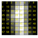
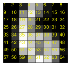
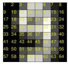
(a) mean images of “1”, “6” and “9”

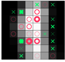
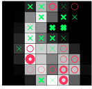
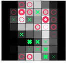
(b) AdaBoost.ECC

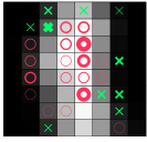
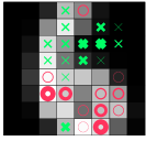
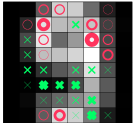
(c) MultiBoost-hinge

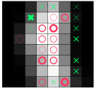
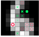
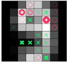
(d) MultiBoost-exp

Figure 1: Plot (a) shows the mean images of the samples belonging to digits “1”, “6” and “9”. Each block is a feature and is numerically indexed. The remaining plots illustrate the classification models trained on this data set by (b) AdaBoost.ECC, (c) MultiBoost-hinge and (d) MultiBoost-exp. Red circles indicate that weak classifiers on these features should take large values; Green crosses indicate small values should be taken on these features in order to make correct classification. The width of a mark is proportional to the weight of the stump. We can see that MultiBoost-hinge is slightly better than AdaBoost.ECC, e.g., on the $43$-th and $21$-th features.

We first performed a few sets of experiments to compare MultiBoost${}^{\,\ell_{1}}$ with previous multi-class boosting algorithms. For fair comparison, we focus on the multi-class algorithms using binary weak learners, including AdaBoost.MO and AdaBoost.ECC, which are still considered as the state-of-the-art. For AdaBoost.MO, the error-correcting output codes are introduced to reduce the primal problem into multiple binary ones; for AdaBoost.ECC, the binary partitioning is made at each iteration by using the “random-half” method, which has been experimentally proven better than the optimal “max-cut” solution Li (2006). Decision stumps are chosen as the weak classifiers for all boosting algorithms, due to its simplicity and the controlled complexity of the weak learner.

Convex optimization problems are involved in MultiBoost-hinge and MultiBoost-exp. To solve them, we use the off-the-shelf Mosek convex optimization package, which provides solutions for both primal and dual problems simultaneously with its interior-point Newton method. We also need to set the regularization parameter $\nu$ for these two algorithms using cross validation. For each run, a five-fold cross validation is carried out first to determine the best $\nu$. Notice that the loss functions in MultiBoost-hinge and MultiBoost-exp may have different scales, we choose the parameter from $\{10^{-4}$, $10^{-3}$, $5\cdot 10^{-3}$, $0.01$, $0.02$, $0.04$, $0.05\}$ for the former, and the candidate pool $\{10^{-8}$, $10^{-7}$, $5\cdot 10^{-7}$, $8\cdot 10^{-7}$, $10^{-6}$, $2\cdot 10^{-6}$, $4\cdot 10^{-6}$, $8\cdot 10^{-6}$, $10^{-5}\}$ for the latter.

Toy data

In the first experiment, we make the comparison on a toy data set, which consists of 4 clusters of planar points. Each cluster has 50 samples, which are drawn from their respective normal distribution. As shown in Figure 2(a), the centers of the circles indicate where their means are, and the radii depict the different deviations. We run the boosting algorithms on this toy data set and plot the decision boundaries on the $x$-$y$ plane. Figures 2(b)-(e) illustrate the results when the number of training iterations is set to be $100$. In this case, it is hard to state which model is better. However, if we increase the iteration to $5000$ times, the planes in (f) and (g) are apparently over segmented by AdaBoost.MO and AdaBoost.ECC. On the contrary, the decision boundaries of (h) MultiBoost-hinge and (i) MultiBoost-exp seem closer to the true decision boundary. Unlike the others, models trained by AdaBoost.MO are more complex, since this learning method assembles $\ell$ weak classifiers rather than one at each iteration if $\ell$-length codewords are used. Empirically we see that AdaBoost.ECC also seems susceptible to over-fitting.

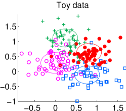
(a) data

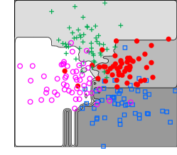
(b) AdaBoost.MO, 100 iterations

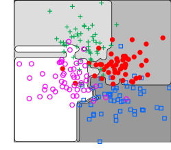
(c) AdaBoost.ECC, 100 iterations

(d) MultiBoost-hinge, 100 iterations

(e) MultiBoost-exp, 100 iterations

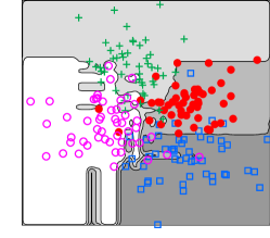
(f) AdaBoost.MO, 5000 iterations

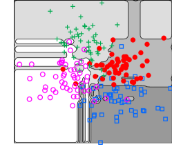
(g) AdaBoost.ECC, 5000 iterations

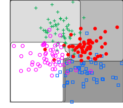
(h) MultiBoost-hinge, 5000 iterations

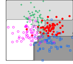
(i) MultiBoost-exp, 5000 iterations

Figure 2: Figure (a) shows a toy data set, which contains 4 classes and a total of 200 sample points. Boosting algorithms are trained on this set using decision stumps. Plots (b)-(e) illustrate the decision boundaries made by (b) AdaBoost.MO, (c) AdaBoost.ECC, (d) MultiBoost-hinge and (e) MultiBoost-exp with the number of training iterations being $100$. For comparison, plots (f)-(i) illustrate the decision boundaries of these algorithms, respectively, when the number of iterations is $5000$. (f) and (g) apparently suffer from over-fitting.

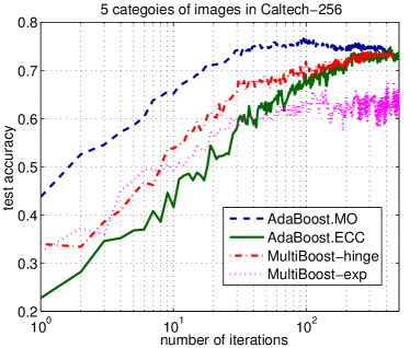
Figure 3: Test accuracy curves of four boosting algorithms on 5 categories of Caltech-256 images. The weak classifiers are decision stumps and the number of training iterations is $500$. The average results of $10$ runs are reported. Each run randomly selects $75\%$ data for training and the other $25\%$ for test.

UCI data sets

Next we test our algorithms on $7$ data sets collected from UCI repository. Samples are randomly divided into $75\%$ for training and $25\%$ for test, no matter whether there is a pre-specified split or not. Each data set is run $10$ times and the average results of test error are reported in Table 1. The maximum number of iterations is set to $500$. Almost all the algorithms converge before the maximum iteration. Again the regularization parameter is determined by 5-fold cross validation.

Table 1 reports the results. The conclusion that we can draw on this experiment is: 1) Overall, all the algorithms achieve comparable accuracy. 2) our algorithms are slightly better in terms of generalization ability than the other two on $5$ out of $7$ data sets. MultiBoost-exp outperforms others in $4$ data sets. 3) Also note that the performance MultiBoost-hinge is more stable than MultiBoost-exp, which may be due to the fact that the hinge loss is less sensitive to noise than the exponential loss.

dataset	AdaBoost.MO	AdaBoost.ECC	MultiBoost-hinge	MultiBoost-exp
thyroid	0.005$\pm$0.001	0.005$\pm$0.001	0.005$\pm$0.001	0.004$\pm$0.001
dna	0.059$\pm$0.005	0.064$\pm$0.005	0.057$\pm$0.007	0.061$\pm$0.004
wine	0.036$\pm$0.025	0.034$\pm$0.029	0.032$\pm$0.018	0.030$\pm$0.029
iris	0.062$\pm$0.017	0.073$\pm$0.021	0.068$\pm$0.022	0.057$\pm$0.022
glass	0.232$\pm$0.047	0.242$\pm$0.053	0.234$\pm$0.046	0.315$\pm$0.086
svmguide2	0.213$\pm$0.039	0.214$\pm$0.030	0.222$\pm$0.052	0.206$\pm$0.040
svmguide4	0.192$\pm$0.018	0.191$\pm$0.018	0.207$\pm$0.018	0.214$\pm$0.027

Table 1: Test errors of four boosting algorithms on UCI data sets. The average results of 10 repeated tests are reported. Weak classifiers are decision stumps. MultiBoost-exp is the best on 4 out of 7 data sets.

Handwriting digits recognition

To further examine the effectiveness of our algorithms, We have conducted another experiment on a handwritten digits data set, which is also from UCI repository. The original data set contains $5620$ digits written by a total of $43$ people on $32\times 32$ bitmaps. Then the bitmaps are divided into $4\times 4$ non-overlapping blocks, and an $8\times 8$ descriptor is generated by calculating the sum of $0$-$1$ pixels in each block. For ease of exposition, only $3$ distinct digits of “1”, “6” and “9” are chosen for classification. Figure 1(a) illustrates the mean images of their training data examples of the three digits. The index of each block (feature) is also printed on Figure 1(a) for the convenience of exposition.

We train multi-class boosting on this data set. The number of maximum training iterations is set to $500$. $75\%$ data are used for training, and the rest for test. Again $5$-fold cross validation is used. We still use decision stumps as the weak classifiers. Boosting learning with decision stumps implies that we select features at the same time. In other words, decision stumps select most discriminative blocks for classifying these digits. The four compared algorithms have similar performances on this test with nearly $98\%$ test accuracy. We plot the models of AdaBoost.ECC, MultiBoost-hinge and MultiBoost-exp in Figures 1(b)-(d). AdaBoost.MO can be hardly illustrated as it involves a multi-dimensional coding scheme. Notice that a decision stump divides the value range of the feature into two parts, on which there are necessarily two different attributions, we use red circles and green crosses to represent the positive and negative parts. For example, if a decision stump on the $10$-th feature is $x_{10}>\tau$ and assigns a set of weights $\{0.5,0.2,0.8\}$ to three labels, we mark $10$-th block in the third digit image with a red circle, and $10$-th block in the second digit with a green cross; if the stump is $x_{10}<\tau$ with the same weights, we do the opposite marks. In other words, red circles indicate the decision stumps should take bigger values on these blocks, while green crosses indicate these classifiers should take some values as small as possible. The width of a mark stands for the minimal margin defined in Equation (10), that is, in the $i$-th digit, the width is proportional to $h({\boldsymbol{x}}){\boldsymbol{w}}_{y_{i}}-\max\{h({\boldsymbol{x}}){\boldsymbol{w}}_{r}\}$, $\forall r\neq y_{i}$. Some features may be selected multiple times, which divide the value range into several segments. In this case, we neglect all the middle parts.

Figure 4: Some examples of correctly classified (top two rows) and misclassified (bottom row) images by MultiBoost-hinge. The categories are “cartman”, “headphones”, “iris”, “paperclip” and “skunk”. The accuracy of this test is $71.2\%$. No image is falsely classified into the category of “paperclip”.

Clearly, all the results of three algorithms on feature selection make sense. Most discriminative features are tagged with circles or crosses. Some blocks that contain significant information on luminance are tagged with thick marks, such as the $22$-th and $43$-th features in digit “6”, and the $22$-th and $11$-th in “9”. If taking a close look at the figure, we can find MultiBoost-hinge is slightly better than AdaBoost.ECC. For example, on the $43$-th feature the green cross should be marked on digit “9” instead of “1”. Also in “1”, the $21$-th feature should be tagged with a relatively thicker circle. However, MultiBoost-exp’s results are not as meaningful as MultiBoost-hinge.

Object recognition on a subset of Caltech-$256$

Finally, we test our algorithms on the data set of Caltech-$256$, which is one of the most popular multi-class benchmarks. We randomly select $5$ categories of images. $75\%$ of them are randomly selected for training and the other $25\%$ for test. A descriptor of $1000$ dimensions is used, which combines quantized color and texture local invariant features (also called visterms (Quelhas and Odobez, 2006)). The maximum number of iterations is still set to $500$. The averaged test accuracies of $10$ runs are reported in Figure 3. Again, we use the simplest decision stumps as weak classifiers. We can see that all the four boosting algorithms perform similarly, except that MultiBoost-exp performs worse than the other three. It may be due to the fact that we have not fine tuned the cross validation parameter. We show some images that are correctly classified and falsely classified by MultiBoost-hinge in Figure 4.

3.2 MultiBoost${}^{\,\rm group}$

Next we evaluate our mixed-norm regularized boosting algorithms. We mainly use the $\ell_{1,2}$ regularization since $\ell_{1,\infty}$ delivers similar performance. In order to ensure a fair comparison we evaluate the performance of the proposed algorithms against other multi-class boosting algorithms evaluated previously, along with AdaBoost-SIP (Zhang et al., 2009), JointBoost (Torralba et al., 2007), GradBoost ($\ell_{1}/\ell_{2}$-regularized) (Duchi and Singer, 2009). Note that the last three also try to share features across classes.

Artificial data

We consider the problem of discriminating $6$ object classes on a $2$D plane. Each sample consists of $2$ measurements: orientation and radius. For all classes, the orientation is drawn uniformly between $0$ and $2\pi$. The radius of the first group is drawn uniformly between $0$ and $1$, the radius of the second group between $1$ and $2$, and so on. We generate $50$ samples in the first group, $100$ samples in the second group, $150$ samples in the third group, and so on. The number of training sets is the same as the number of test sets. In this example feature vectors are the vertical and horizontal coordinates of the samples. We train $5$ different classifiers based on the proposed MultiBoost${}^{\,\rm group}$ (hinge loss), AdaBoost.MH (Schapire and Singer, 1999), AdaBoost.ECC (Guruswami and Sahai, 1999) and JointBoost (Torralba et al., 2007). The multi-class classifier is composed of a set of binary decision stumps. For our algorithm, we choose the regularization parameter $\nu$ from $\{10^{-5},10^{-4},10^{-3},10^{-2},10^{-1}\}$. For JointBoost, we set the outermost class (maximal radius) as background. We evaluate $5$ boosting algorithms on this toy data and plot the decision boundary in Figure 5. Table 2 reports some training and test error rates. Our algorithm performs best amongst five evaluated classifiers. We conjecture that the poor performance of JointBoost is due to the small number of background samples in the training data. JointBoost was designed for the task of multi-class object detection where the objective is to detect several classes of objects from background samples. The algorithm might not work well on general multi-class problems. We then repeat our experiment by increasing the number of iterations to $500$, and JointBoost, Adaboost.MH and AdaBoost.ECC still perform poorly on this toy data set compared to our approach.

$\#$ feat.	Ada.ECC	Ada.MH	JointBoost	MultiBoost${}^{\,\ell_{1}}$	MultiBoost${}^{\,\rm group}$
$20$	$0.62/0.68$	$0.48/0.53$	$0.71/0.71$	$0.10/$0.14	$0.10/$0.14
$100$	$0.23/0.33$	$0.17/0.24$	$0.44/0.50$	$0.05/0.13$	$0.03/$0.10
$500$	$0.08/0.20$	$0.09/0.18$	$0.24/0.38$	$0.03/0.10$	$0.02/$0.09

Table 2: Training$/$test errors of a few multi-class boosting methods on the $2$D toy data set. The proposed MultiBoost${}^{\,\rm group}$ with hinge loss performs slightly better than others. See Figure 5 for an illustration.

AdaBoost.ECC

AdaBoost.MH

JointBoost

MultiBoost${}^{\,\ell_{1}}$

MultiBoost${}^{\,\rm group}$

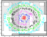
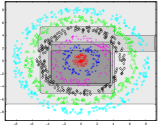
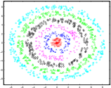
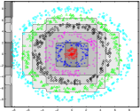
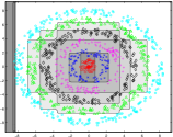
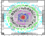
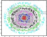
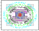
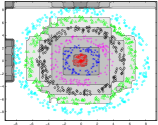
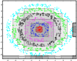
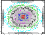
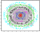
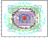
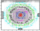
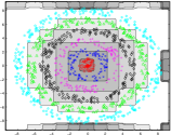
Figure 5: Decision boundaries on a toy data sets, with Top row: $20$ weak classifiers Middle row: $100$ weak classifiers and Bottom row: $500$ weak classifiers. Note that some multi-class algorithms end up with very complicated and multi-modal decision boundaries.

UCI data sets

The second experiment is carried out on some UCI machine learning data sets. Since we are more interested in the performance of multi-class algorithms when the number of classes is large, we evaluate our algorithm on ‘segment’ ($7$ classes), ‘USPS’ ($10$ classes), ‘pendigits’ ($10$ classes), ‘vowel’ ($11$ classes) and ‘isolet’ ($26$ classes). All data instances from ‘segment’ and ‘vowel’ are used in our experiment. For USPS, pendigits and isolet we randomly select $100$ samples from each class. We use the original attributes for USPS ($256$ attributes) and isolet ($617$ attributes). For the rest, we increase the number of attributes by multiplying pairs of attributes. Each data set is then randomly split into two groups: $75\%$ samples for training and $25\%$ for evaluation. In this experiment, we compare MultiBoost${}^{\,\rm group}$ (logistic loss) to AdaBoost.MH (Schapire and Singer, 1999), AdaBoost.ECC (Guruswami and Sahai, 1999) and GradBoost ($\ell_{1}/\ell_{2}$-regularized) (Duchi and Singer, 2009). The regularization parameter is first determined by $5$-fold cross validation.

For GradBoost, we choose the regularization parameter from $\{10^{-4},5\cdot 10^{-4},10^{-3},5\cdot 10^{-3},10^{-2},5\cdot 10^{-2},10^{-1},5\cdot 10^{-1}\}$. For our algorithm, we choose the regularization parameter from $\{10^{-7},5\cdot 10^{-7},10^{-6},5\cdot 10^{-6},10^{-5},5\cdot 10^{-5},10^{-4},5\cdot 10^{-4},10^{-3}\}$. All experiments are repeated $10$ times using the same regularization parameter. The maximum number of boosting iterations is set to $500$. We observe that almost all the algorithms converge earlier than $500$ in this experiment. We plot the mean of test errors versus proportion of features used in Figure 6. These results show that our proposed approach consistently outperforms its competitors. On the ‘segment’ and ‘vowel’ data sets we observe that both MultiBoost${}^{\,\ell_{1}}$ and MultiBoost${}^{\,\rm group}$ perform similarly. We suspect that this is because the number of attributes in both data sets is quite small, and thus that there is little advantage to be gained through feature sharing on these data sets. Our approach often has the fastest convergence rate (note, however, that GradBoost converges faster on the USPS data sets but ends up with a larger test error).

Comparison between GradBoost and our algorithm

GradBoost with mixed-norm regularization (Duchi and Singer, 2009) is similar to the method presented here. The distinction, however, is that our method minimizes the original convex loss function rather than quadratic bounds on this function. The result is that our method is not only more effective, but also more general, as it can be applied not only to the logistic loss function but also to any convex loss function. In addition, our approach shares a similar formulation to standard boosting algorithms, i.e., the way we generate weak learners or update sample weights (dual variables in our algorithm). The algorithm of Duchi and Singer (2009) is rather heuristic and it is not known when the algorithm will converge. Furthermore, GradBoost is more similar to FloatBoost (Li and Zhang, 2004) where the authors introduce a backward pruning step to remove less discriminative weak classifiers. The drawback of pruning is 1) being heuristic and 2) a prolonged training process.

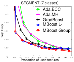
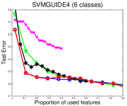
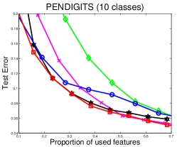
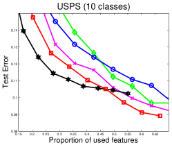
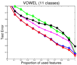
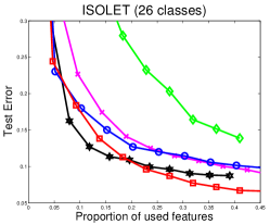
Figure 6: The performance of our algorithm (MultiBoost${}^{\,\rm group}$) compared with various boosting algorithms on several machine learning data sets. The horizontal axis is the fraction of used features and the vertical axis is the test error rate. We observe that group sparsity-based approaches (ours and GradBoost) generally converge faster than other algorithms.

ABCDETC and MNIST handwritten data

The NEC Lab ABCDETC sets consist of $72$ classes (digits, letters and symbols). For this experiment, we only use digits and letters ($10$ digits, $26$ lower cases and $26$ upper cases). We first resize the original images to a resolution of $28\times 28$ pixels and apply a de-skew pre-processing. We then apply a spatial pyramid and extract $3$ levels of HOG features with $50\%$ block overlap. The block size in each level is $4\times 4$, $7\times 7$ and $14\times 14$ pixels, respectively. Extracted HOG features from all levels are concatenated. In total, there are $2,172$ HOG features. For ABCDETC, we randomly select $5$ samples from each class as training sets and $120$ samples from each class as test sets. For MNIST, we randomly select $100$ samples from each class as training sets and used the original test sets of $10,000$ samples. In this experiment, we also compare the performance of MultiBoost${}^{\,\rm group}$ with a fast training variant, MultiBoost${}^{\rm group}_{\text{\sc fast}}$. All experiments are run $10$ times with $500$ boosting iterations and the results are briefly summarized in Table 3. From the table, both MultiBoost${}^{\,\rm group}$ and MultiBoost${}^{\rm group}_{\text{\sc fast}}$ perform best compared to other evaluated algorithms, especially on ABCDETC test sets where the number of classes is large. We observe the fast approach to perform slightly better than MultiBoost${}^{\,\rm group}$. In our work, the advantage of the fast approach compared to MultiBoost${}^{\,\rm group}$ is that the training time can be further reduced by exploiting parallelism in ADMM, as previously mentioned. Table 4 illustrates the feature sharing property of our algorithms. Clearly we can see that the group sparsity regularization indeed encourages sharing features.

	MNIST	ABCDETC
Ada.MH (Schapire and Singer, 1999)	3.0 ($0.2$)	$63.4$ ($1.8$)
Ada.ECC (Guruswami and Sahai, 1999)	$3.1$ ($0.2$)	$70.5$ ($1.1$)
Ada.SIP (Zhang et al., 2009)	$4.4$ ($1.3$)	$62.7$ ($1.2$)
GradBoost (Duchi and Singer, 2009)	$5.3$ ($0.3$)	$73.9$ ($1.3$)
MultiBoost${}^{\,\ell_{1}}$	$3.7$ ($0.2$)	$73.2$ ($0.7$)
MultiBoost${}^{\,\rm group}$	$3.1$ ($0.2$)	$59.1$ ($1.1$)
MultiBoost${}^{\rm group}_{\text{\sc fast}}$	3.0 ($0.3$)	58.2 ($0.9$)

Table 3: Test errors (%) of a few multi-class boosting methods on the MNIST and ABCDETC handwritten data sets. All experiments are run $10$ times with $500$ boosting iterations. The average error mean and standard deviation (in percentage) are reported.

MNIST	‘$0-3$’	‘$4-5$’	‘$6-7$’	‘$8-10$’
MultiBoost${}^{\,\ell_{1}}$	$99.8\%$	$0.2\%$	$0\%$	$0\%$
MultiBoost${}^{\,\rm group}$	$4.5\%$	$48.8\%$	$40.9\%$	$5.8\%$
MultiBoost${}^{\rm group}_{\text{\sc fast}}$	$10.1\%$	$69.9\%$	$19.7\%$	$0.3\%$
ABCDETC	‘$0-15$’	‘$16-30$’	‘$31-45$’	‘$46-62$’
MultiBoost${}^{\,\ell_{1}}$	$99.8\%$	$0.2\%$	$0\%$	$0\%$
MultiBoost${}^{\,\rm group}$	$0\%$	$81.3\%$	$18.7\%$	$0\%$
MultiBoost${}^{\rm group}_{\text{\sc fast}}$	$0\%$	$65.7\%$	$33.5\%$	$0.7\%$

Table 4: The distribution of shared weak classifiers. For example, ‘$8-10$’ indicates that the weak classifier is being shared among $8$ to $10$ classes. The table illustrates the feature sharing property of our algorithms, i.e., one weak classifier is being shared among multiple classes.

Scene recognition

In the next experiment, we compare our approach on the $15$-scene data set used in Lazebnik et al. (2006). The set consists of $9$ outdoor scenes and 6 indoor scenes. There are $4,485$ images in total. For each run, the available data are randomly split into a training set and a test set based on published protocols. This is repeated $5$ times and the average accuracy is reported. In each train/test split, a visual codebook is generated using only training images. Both training and test images are then transformed into histograms of code words. We use CENTRIST of Wu and Rehg (2011) as our feature descriptors. $200$ visual code words are built using the histogram intersection kernel (HIK), which has been shown to outperform $k$-means and $k$-median (Wu and Rehg, 2011). We represent each image in a spatial hierarchy manner (Bosch et al., 2008). Each image consists of $31$ sub-windows. An image is represented by the concatenation of histograms of code words from all $31$ sub-windows. Hence, in total there are $6,200$ dimensional histogram.

Figure 7 shows the average classification errors. We observe that both MultiBoost${}^{\,\rm group}$ and MultiBoost${}^{\,\ell_{1}}$ converge quickly in the beginning. However, MultiBoost${}^{\,\rm group}$ has a better overall convergence rate. We also observe that both (MultiBoost${}^{\,\rm group}$ and MultiBoost${}^{\rm group}_{\text{\sc fast}}$), have the lowest test error compared to other algorithms evaluated. We also apply a multi-class SVM to the above data set using the LIBSVM package (Chang and Lin, 2011) and report the recognition results in Table 5. SVM with $6,200$ features achieves an average accuracy of $76.30\%$ (linear) and $81.47\%$ (non-linear). Our results indicate that both proposed approaches achieve a comparable accuracy to non-linear SVM while requiring less number of features ($77.8\%$ accuracy for MultiBoost${}^{\,\rm group}$ with $1000$ features and $79.2\%$ accuracy for MultiBoost${}^{\rm group}_{\text{\sc fast}}$).

methods	$\#$ features used	accuracy ($\%$)
SAMME† (Zhu et al., 2009)	$1000$	$70.9$ ($0.40$)
JointBoost† (Torralba et al., 2007)	$1000$	$72.2$ ($0.70$)
MultiBoost${}^{\,\ell_{1}}$	$1000$	$76.0$ ($0.48$)
AdaBoost.SIP (Zhang et al., 2009)	$1000$	$75.7$ ($0.10$)
AdaBoost.ECC (Guruswami and Sahai, 1999)	$1000$	$76.5$ ($0.67$)
AdaBoost.MH (Schapire and Singer, 1999)	$1000$	$77.6$ ($0.59$)
MultiBoost${}^{\,\rm group}$	$1000$	$77.8$ ($0.77$)
MultiBoost${}^{\rm group}_{\text{\sc fast}}$	1000	79.2 ($0.82$)
Linear SVM	$6200$	$76.3$ ($0.88$)
Nonlinear SVM (HIK)	6200	81.4 ($0.60$)

Table 5: Recognition rate of various algorithms on Scene$15$ data sets. All experiments are run $5$ times. The average accuracy mean and standard deviation (in percentage) are reported. Results marked by ${\dagger}$ were reported in Zhang et al. (2009).

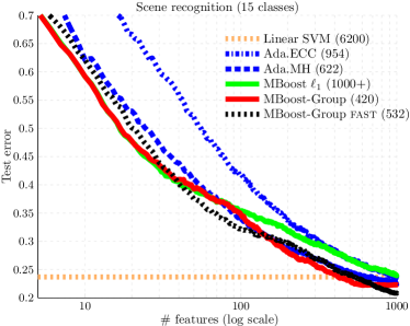
Figure 7: Performance of different classifiers on the scene recognition data set. We also report the number of features required to achieve similar results to linear multi-class SVM. Both of our methods (MultiBoost${}^{\,\rm group}$ and MultiBoost${}^{\rm group}_{\text{\sc fast}}$) outperform other evaluated boosting algorithms.

Traffic sign recognition

We evaluate our approach on the recent German traffic sign recognition benchmark. Data sets consist of $43$ classes with more than $50,000$ images in total. We randomly select $100$ samples from each class to train our classifier. We use the provided test set to evaluate the performance of our classifiers ($12,569$ images). All training images are scaled to $40\times 40$ pixels using bilinear interpolation. Three different types of pre-computed HOG features are provided ($6,052$ features). We combine all three types together. We also make use of histogram of hue values ($256$ bins). Hence, there is a total of $6,308$ features. The results of different classifiers are shown in Figure 8. Our proposed classifier outperforms other evaluated classifiers. As a baseline, we train a multi-class SVM using LIBSVM (Chang and Lin, 2011). SVM achieves $93.05\%$ (using $6,308$ features) while our classifier achieves $95.62\%$ for MultiBoost${}^{\,\rm group}$ and $95.42\%$ for MultiBoost${}^{\rm group}_{\text{\sc fast}}$ with a much smaller set of features ($500$ features). Note that an overfitting behavior is observed for MultiBoost${}^{\,\ell_{1}}$.

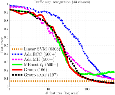
Figure 8: Performance of different classifiers on traffic sign recognition data sets. We also report the number of features needed to achieve a similar accuracy to the linear SVM. Both of our methods outperform other multi-class methods in terms of the test error.

4 Conclusion

In this work, we have presented a direct formulation for multi-class boosting. We derive the Lagrange dual of the formulated primal optimization problem. Based on the dual problem, we are able to design fully-corrective boosting using the column generation technique. At each iteration, all weak classifiers’ weights are updated. We then generalize our approach and propose a new feature-sharing multi-class boosting method. The proposed boosting is based on the primal-dual view of the group sparsity regularized optimization. Various experiments on a few different data sets demonstrate that our direct multi-class boosting achieves competitive test accuracy compared with other existing multi-class boosting.

Future research topics include how to efficiently solve the convex optimization problems of the proposed multi-class boosting. Conventional multi-class boosting do not need to solve convex optimization at each step and thus much faster. We also want to explore the possibility of structural learning with boosting by extending the proposed multi-class boosting framework.

References

- Bosch et al. (2008) A. Bosch, A. Zisserman, and X. Munoz. Scene classification using a hybrid generative/discriminative approach. IEEE Trans. Pattern Anal. & Mach. Intelligence, 30(4):712 – 727, 2008.
- Boyd and Vandenberghe (2004) S. Boyd and L. Vandenberghe. Convex Optimization. Cambridge University Press, 2004.
- Boyd et al. (2011) S. Boyd, N. Parikh, E. Chu, B. Peleato, and J. Eckstein. Distributed optimization and statistical learning via the alternating direction method of multipliers. Foundations & Trends in Mach. Learn., 3(1), 2011.
- Chang and Lin (2011) C-C. Chang and C.-J. Lin. LIBSVM: A library for support vector machines. ACM Trans. Intell. Sys. & Tech., 2(3), 2011.
- Chapelle and Keerthi (2008) O. Chapelle and S. S. Keerthi. Multi-class feature selection with support vector machines. In Proc. American Stat. Assoc., 2008.
- Crammer and Singer (2001) K. Crammer and Y. Singer. On the algorithmic implementation of multiclass kernel-based vector mchines. J. Mach. Learn. Research, 2:265–292, 2001.
- Crammer and Singer (2002) K. Crammer and Y. Singer. On the learnability and design of output codes for multiclass problems. Mach. Learn., 47(2):201–233, 2002.
- Daniely et al. (2012) A. Daniely, S. Sabato, and S. S. Shwartz. Multiclass learning approaches: A theoretical comparison with implications. In Proc. Adv. Neural Info. Process. Syst., 2012.
- Demiriz et al. (2002) A. Demiriz, K. P. Bennett, and J. Shawe-Taylor. Linear programming boosting via column generation. Mach. Learn., 46(1-3):225–254, 2002. ISSN 0885-6125.
- Dietterich and Bakiri (1995) T.G. Dietterich and G. Bakiri. Solving multiclass learning problems via error-correcting output codes. J. Artificial Intelligence Research, 2:263–286, 1995.
- Duchi and Singer (2009) J. Duchi and Y. Singer. Boosting with structural sparsity. In Proc. Int. Conf. Mach. Learn., 2009.
- Elisseeff and Weston (2001) A. Elisseeff and J. Weston. A kernel method for multi-labelled classification. In Proc. Adv. Neural Info. Process. Syst., pages 681–687. MIT Press, 2001.
- Freund and Schapire (1997) Y. Freund and R. E. Schapire. A decision-theoretic generalization of on-line learning and an application to boosting. J. Computer & System Sciences, 55(1):119–139, 1997.
- Guruswami and Sahai (1999) V. Guruswami and A. Sahai. Multiclass learning, boosting, and error correcting codes. In Proc. Annual Conf. Learn. Theory, pages 145–155, 1999.
- Lazebnik et al. (2006) S. Lazebnik, C. Schmid, and J. Ponce. Beyond bags of features: Spatial pyramid matching for recognizing natural scene categories. In Proc. IEEE Conf. Comp. Vis. Patt. Recogn., 2006.
- Li (2006) L. Li. Multiclass boosting with repartitioning. In Proc. Int. Conf. Mach. Learn., pages 569–576, 2006.
- Li and Zhang (2004) S. Z. Li and Z. Zhang. FloatBoost learning and statistical face detection. IEEE Trans. Pattern Anal. & Mach. Intelligence, 26(9):1112–1123, 2004.
- Mason et al. (2000) L. Mason, J. Baxter, P. Bartlett, and M. Frean. Boosting algorithms as gradient descent. In Proc. Adv. Neural Info. Process. Syst., pages 512–518. MIT Press, 2000.
- MOSEK (2012) MOSEK. The MOSEK optimization tools manual (version 6.0), 2012. URL http://www.mosek.com/.
- Quelhas and Odobez (2006) P. Quelhas and J. M. Odobez. Natural scene image modeling using color and texture visterms. Image & Video Retrieval, pages 411–421, 2006.
- Schapire and Singer (1999) R. Schapire and Y. Singer. Improved boosting algorithms using confidence-rated prediction. Mach. Learn., 37(3):297–336, 1999.
- Schapire et al. (1998) R. Schapire, Y. Freund, P. Bartlett, and W. Lee. Boosting the margin: A new explanation for the effectiveness of voting methods. Ann. Statist., 26(5):1651–1686, 1998.
- Schapire (1997) R. E. Schapire. Using output codes to boost multiclass learning problems. In Proc. Int. Conf. Mach. Learn., pages 313–321, 1997.
- Shen and Li (2010) C. Shen and H. Li. On the dual formulation of boosting algorithms. IEEE Trans. Pattern Anal. & Mach. Intelligence, 32(12):2216–2231, 2010.
- Torralba et al. (2007) A. Torralba, K. P. Murphy, and W. T. Freeman. Sharing visual features for multiclass and multiview object detection. IEEE Trans. Pattern Anal. & Mach. Intelligence, 29(5):854–869, 2007.
- Tsochantaridis et al. (2005) I. Tsochantaridis, T. Joachims, T. Hofmann, and Y. Altun. Large margin methods for structured and interdependent output variables. J. Mach. Learn. Research, 6:1453–1484, 2005.
- Viola and Jones (2004) P. Viola and M. J. Jones. Robust real-time face detection. Int. J. Comp. Vis., 57(2):137–154, 2004.
- Weston and Watkins (1999) J. Weston and C. Watkins. Support vector machines for multi-class pattern recognition. In Proc. Euro. Symp. Artificial Neural Networks, volume 4, pages 219–224, 1999.
- Wu and Rehg (2011) J. Wu and J. M. Rehg. CENTRIST: A visual descriptor for scene categorization. IEEE Trans. Pattern Anal. & Mach. Intelligence, 33(8):1489–1501, 2011.
- Wu et al. (2004) T.-F. Wu, C.-J. Lin, and R C. Weng. Probability estimates for multi-class classification by pairwise coupling. J. Mach. Learn. Research, 5:975 – 1005, 2004.
- Zhang et al. (2009) B. Zhang, G. Ye, Y. Wang, J. Xu, and G. Herman. Finding shareable informative patterns and optimal coding matrix for multiclass boosting. In Proc. IEEE Int. Conf. Comp. Vis., 2009.
- Zhu et al. (2009) J. Zhu, S. Rosset, H. Zou, and T. Hastie. Multi-class AdaBoost. Stat. & its interface, 2:349–360, 2009.