Two channel orbital Kondo effect in quantum dot with SO(n) symmetry

Abstract

A scenario for the formation of non-Fermi-liquid (NFL) Kondo effect (KE) with spin variable enumerating Kondo channels is suggested and worked out. In doubly occupied symmetric triple quantum dot within parallel geometry, the NFL low-energy regime arises provided the device possesses both source-drain and left-right parity. Kondo screening follows a multistage renormalization group mechanism: reduction of the energy scale is accompanied by the change of the relevant symmetry group from $SO(8)$ to $SO(5)$. At low energy, three phases compete: 1) under-screening spin triplet (conventional) KE; 2) spin singlet potential scattering; 3) NFL phase where the roles of spin and orbital degrees of freedom are swapped.

I Introduction

The physics of two-channel Kondo effect (2CKE) that is marked by non-fermi liquid (NFL) behavior at low temperatures has been with us for more than three decades.NoBla80 . Complex quantum dots (CQD) coupled to metallic leads via several channels may be considered as candidates for possible realization of multichannel KE. The simplest object of this kind is a double quantum dot coupled to two source and two lead electrodes.Hoza02 ; Eto05 ; Lim06 ; Trocha10 The generic $SU(4)$ symmetry of this device is realized by two spin 1/2 projections and two orbital states of an electron in a double quantum dot. This configuration paves the way to observation of the $SU(4)$ Kondo effect for four-fold degenerate ground state or at least for the orbital $SU(2)$ KE realized only by orbital degrees. It should be noted that unavoidable interference between different channels emerging in cotunneling process through CQD turns the $SU(4)$ fixed point to be unstable.Lim06 As a result of this inteference one of the two channels becomes dominant at low temperatures, resulting in an $SU(4)\rightarrow SU(2)$ crossover (see Ref. Tetta12, and references therein for experimental realization of these effects in carbon nanotubes and multivalley silicon quantum dots).

In order to realize 2CKE for odd occupation in double quantum dot structures, one more tunneling channel should be involved in electron tunneling processes. However the NFL regime is still elusive due to the same channel anisotropy emerging from inter-channel cotunneling processes. To remedy this instability, a suppression of interchannel cotunneling is attempted, using special design of the CQD. Apparently, the most successful attempt is realized in double quantum dot (DQD),Potok07 where the interference is suppressed by Coulomb blockade. Another design which allows one to (at least) approach the elusive two-channel fixed point was suggested in Ref. KKA03, , based on a structure composed of triple quantum dot (TQD) in a serial geometry (Fig. 1, left panel). Here, the strong Coulomb blockade in the central dot minimizes (but does not completely eliminate) interchannel interference.

Yet another approach for achieving NFL two-channel Kondo regime is to swap the roles of charge and spin variables, i.e., to treat orbital or charge fluctuations as pseudospin variables causing Kondo screening, whereas spin projection quantum numbers serve as different channels.Kondo76 ; WlaZa83 ; MuFi96 ; MuFi97 ; CoZa98 The proposal was based on the idea that the orbital degrees of freedom of heavy spinless particles in a two-well or three-well potential trap may be converted into pseudospin variables, and the latter may play part of the source of Kondo screening, while the spin projections of conduction electrons enumerate the screening channels. This idea was subject to criticism.KaPro86 ; Aleiner01 ; AlContr02 In these systems, pseudospin-flip is a generic tunneling process with a characteristic (long) time $t_{\rm tun}$, unlike real spin flip processes which are practically instantaneous. As a result the ultraviolet cutoff for Kondo effect is the energy $\sim\hbar/t_{\rm tun}$. This energy is of the order of the distance to the next excited level in two-well potential. The latter interval is much smaller than the energy scale $\varepsilon_{F}$ for ”light” electrons. As a result the energy interval available for the formation of the logarithmic singularity is too narrow and the resulting Kondo temperature is very small $T_{K}\ll\Delta$ where $\Delta$ is the depth of the occupied level in the well relative $\varepsilon_{F}.$ Thus the strong coupling regime remains in fact unattainable as far as two-level systems in heavy particles serve as pseudospin. Some theoretical counter-arguments have been offered later,Zar05 whereas features of NFL behavior were found in the electrical resistivity of glassy ThAsSe single crystal.Cich Thus, the question of whether 2CKE can be unambiguously realized in two-level systems is still under discussion (see also Ref. Delft, ).

Natural and artificial nano-objects provide their own mechanisms of two-channel Kondo tunneling assisted by pseudospin excitations. One such mechanism was proposed for a ”quantum box” connected to a lead by a single-mode point contact. Matv95 ; LebShil01 In this case the relevant operator which logarithmically scales the crossover from the high temperature to the low-temperature region is the capacitance $C(T)\sim\ln(T/T_{K})$. In another model with $SU(3)$ dynamical symmetry the excited state with parity-degenerate rotational levels $(m=\pm 1)$ may cross the $m=0$ level due to interaction with a bath and thus become the source of orbital KE with spin playing the part of a tunneling channel. Arnold07 One more possibility of realizing 2CKE was discussed recentlyLaw10 for a quantum dot coupled to two helical edge states of a 2D topological insulator.

II Model

In this work we offer a relatively simple realization of over-screened orbital Kondo effect where the two-channel regime is realized by two spin projections. The proposed device is composed of a doubly occupied TQD in contact with two terminals within parallel geometry KKA03 . It will be shown that the present model is free of the shortcomings pointed out in Refs. KaPro86, ; Aleiner01, ; AlContr02, because the role of higher excited levels is completely different. Experimentally, this configuration may be realized in triangular arrangement of vertical dots Amaha09 (see Fig 1, right panel).

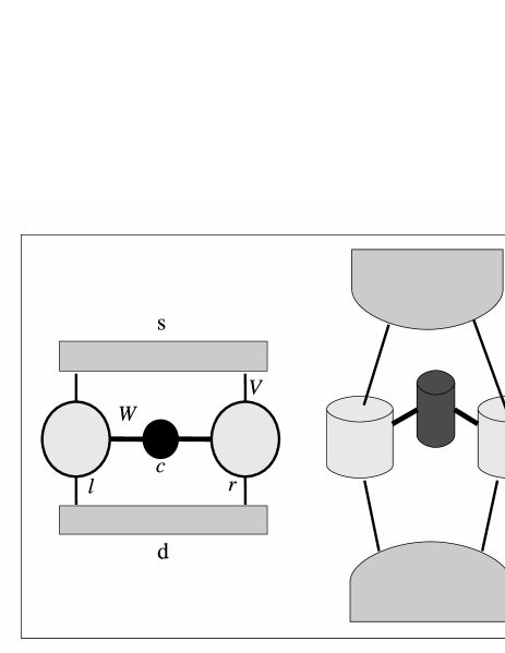
Figure 1: Axially symmetric triple quantum dot in planar (left panel) and vertical (right panel) geometries.

The starting point is the usual Anderson-like tunneling Hamiltonian,

$$H=H_{d}+H_{b}+H_{db}$$ (1)

where

$$H_{d}=\sum_{\lambda=\sigma,\Lambda}E_{\lambda}|\lambda\rangle\langle\lambda|$$

$$H_{b}=\sum_{i=l,r}\sum_{k\sigma}\sum_{a=e,o}\varepsilon_{k}c^{\dagger}_{iak\sigma}c_{iak\sigma}$$ (2)

$$H_{\rm tun}=\sqrt{2}\sum_{ik\sigma\Lambda}\left(\bar{\sigma}V_{\Lambda}c^{{\dagger}}_{iek\sigma}|\bar{\sigma}\rangle\langle\Lambda|+{\rm H.c.}\right).$$

We consider the configuration possessing both left-right ($l$-$r$) and source-drain ($s$-$d$) symmetry. The operators $c^{{\dagger}}_{iak\sigma}$=$(c^{{\dagger}}_{isk\sigma}\pm c^{{\dagger}}_{idk\sigma})/\sqrt{2}$ are even and odd combinations of source and drain electron operators. The latter combinations do not enter $H_{\rm tun}$.Eto05 ; Dynsym The TQD is doubly occupied in the ground state, and only singly occupied states are involved in cotunneling processes. The corresponding eigenstates of the isolated TQD $|\lambda\rangle$ are denoted as $|\sigma\rangle$ and $|\Lambda\rangle$ for the TQD occupied by $N$=1 (spin doublets), and $N$=2 (spin triplets and singlets) electrons respectively.

The low-energy spectrum $E_{\Lambda}$ of the isolated doubly occupied TQD consists of two singlets $E_{Si}$ and two spin triplets $E_{Ti}$ ($i=g,u$ for even and odd combinations of $l$ (left) and $r$(right) states)

$$E_{S_{g}}=\tilde{\varepsilon}-\frac{2W^{2}}{\Delta}-\frac{2W^{2}}{\Delta+Q}-\frac{4W^{2}}{\varepsilon_{c}+Q_{c}-Q_{ic}-\varepsilon},$$

$$E_{T_{u}}=\tilde{\varepsilon}-\frac{2W^{2}}{\Delta},$$

$$E_{S_{u}}=\tilde{\varepsilon}-\frac{2W^{2}}{\Delta+Q},$$

$$E_{T_{g}}=\tilde{\varepsilon},$$ (3)

with $\Delta=\varepsilon-\varepsilon_{c}-Q_{ic}$ (see Appendix A for detailed calculation of these eigenstates and the corresponding eigenfunctions $|\Lambda\rangle$ of the Hamiltonian $H_{d}$).

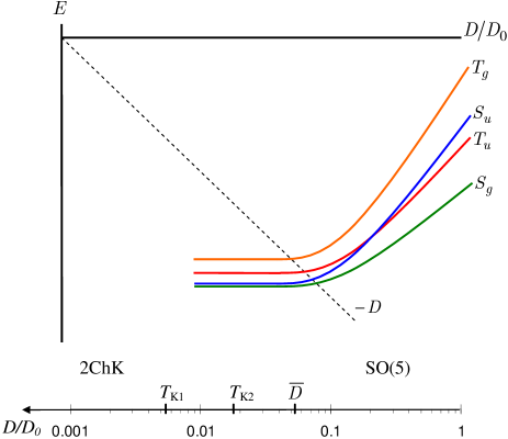
Figure 2: (Color online) Upper panel: Energy levels in doubly occupied TQD renormalized within a scaling procedure. Lower panel: Logarithmic energy scale for a crossover from SO(5) to two-channel KE as a function of scaling parameter $\eta=\ln D_{0}/D$.

Within the energy scale of the bandwidth $D$ (exceeding the width of this multiplet) the spectrum of the isolated TQD is characterized by $SO(8)$ dynamical symmetry. Dynamical symmetry group characterizes the symmetry of the interlevel transitions rather than the symmetry of the Hamiltonian. These transitions involve not only the states belonging to the same irreducible representation characterizing the symmetry of the Hamiltonian but also the processes connecting non-degenerate states belonging to different group representations (see Dynsym for a regular description of dynamical symmetries). Mathematically, dynamical symmetry group of any quantum mechanical system is a group such that all the states of interest are contained in a single irreducible representation of the group. In our case these states are two singlets and two triplets involved in the scaling renormalization (Fig. 2). The dynamical symmetry group is formed by linear combinations of the operators $X^{\lambda\lambda^{\prime}}=|\lambda\rangle\langle\lambda^{\prime}|$ generating the spectrum of the Hamiltonian $H_{d}$. Haldane renormalization Dynsym ; KA01 ; KKA04 ; Hald78 implies that all the levels flow downwards with scaling invariants,

$$E^{*}_{\Lambda}=E_{\Lambda}(D)-\pi^{-1}\Gamma_{\Lambda}\ln(D/\Gamma_{\Lambda}).$$ (4)

Here $\Gamma_{\Lambda}=\pi\rho_{0}|V_{\Lambda}|^{2}$ is the tunneling rate for the state $|\Lambda\rangle$, $\ln(D/D_{0})\equiv\eta$ is the scaling variable and $D_{0}$ is the conduction bandwidth $-D_{0}/2\leq\varepsilon_{k}\leq D_{0}/2$. The renormalization rates $\Gamma_{\Lambda}/\pi$ depend crucially on $\Lambda$, and the scaling trajectories $E_{\Lambda}(D)$ intersect as in Fig. 2 due to the inequality $\Gamma_{T_{g}}>\Gamma_{S_{u}}>\Gamma_{T_{u}}>\Gamma_{S_{g}}$ (see Appendix A for details). Various scenarios of multistage Kondo effect are possible, including that illustrated by the flow diagram of Fig. 2, where the level $E_{S_{u}}$ crosses level $E_{T_{u}}$ before the level $E_{T_{g}}$ ”overtakes” both of them.foot1 There is a window of input parameters, where the orbital KE emerges due to nearly degenerate orbital doublet/spin singlet forming as a result of Haldane flow at $D\approx\bar{D}$, where charge fluctuations are frozen. At this stage, an application of the Schrieffer-Wolff (SW) transformation generates the effective spin Hamiltonian for $N=2$ channels, and further RG transformation follows Anderson’s poor-man scaling procedure for renormalization of the exchange constants.And70

III From SO(5) spin Kondo effect to two-channel orbital Kondo effect

The full $SO(8)$ spin Hamiltonian $H_{\rm SW}$ is derived in Ref. KKA04, . From Fig. 2 we conclude that the poor-man scaling procedure should take into account the evolution of dynamical symmetry along the chain $SO(8)\to SO(5)\to{\rm orbital}~{}SU(2)$. To illustrate the key points of transformation from spin KE to orbital KE, we consider the simplified picture, where only one of the two triplets is taken into account, i.e., write down the spin Hamiltonian pertaining to the part relevant to the KE for the $SO(5)$ multiplet composed of one triplet $T_{u}$ and two singlets $S_{u}$ and $S_{g}$. When the two singlets $|S_{u}\rangle,|S_{g}\rangle$ and the triplet $|T_{u},\mu\rangle$ (where $\mu=1,0,\bar{1}$ are the projections of the spin $S=1$ along a given axis), are almost degenerate, the effective low-energy Hamiltonian can be written as a sum of spin and orbital parts:

$$H_{\rm eff} = H_{\rm spin}+H_{\rm orb}.$$ (5)

The first term $H_{\rm spin}$ is generated at the first stage of full Haldane-Anderson scaling procedure. The second term $H_{\rm orb}$ arises only provided the two lowest states in the renormalized Hamiltonian $H_{d}$ are spin singlets (see below). $H_{\rm spin}$ contains twelve coupling constants (39) (see Appendix B for this derivation), however only three of them are relevant, and the Kondo temperature can be identified from the reduced effective Hamiltonian

$$H_{\rm spin}=\sum_{\mu}{\bar{E}}_{T_{u}}X^{T_{u}\mu,T_{u}\mu}+\sum_{\eta=u,g}{\bar{E}}_{S_{\eta}}X^{S_{\eta}S_{\eta}}+$$ (6)

$$J_{1}{\bf S}_{u}\cdot{\bf s}_{uu}+J_{2}{\bf R}_{u}\cdot{\bf s}_{uu}+J_{3}({\bf R}_{ug}^{(1)}\cdot{\bf s}_{gu}+{\bf R}_{gu}^{(2)}\cdot{\bf s}_{ug}).$$

The coupling constants $J_{i}$ $(i=1-3)$ are defined as:

$$J_{1}=\frac{\alpha_{T}^{2}V^{2}}{\varepsilon_{F}-\varepsilon},\ \ \ \ \ \ \ \ J_{2}=-\frac{\alpha_{u}\alpha_{T}V^{2}}{\varepsilon_{F}-\varepsilon},$$

$$J_{3}=-\frac{\alpha_{g}\alpha_{T}V^{2}}{\varepsilon_{F}-\varepsilon},$$

(see Eqs. (A) for definition of the parameters $\alpha$ and $\beta$). The levels $\bar{E}_{\Lambda}$ are renormalized in accordance with Eq. (4). The group generators forming the $o_{5}$ algebra are three vectors ${\bf S}_{u},{\bf R}_{u},{\bf\tilde{R}}={\bf{R}}^{(1)}_{ug}+{\bf{R}}^{(2)}_{gu}$ and the scalar $A$:

$$S^{+}_{u} = \sqrt{2}(X^{1_{u}0_{u}}+X^{0_{u}\bar{1}_{u}}),\ S^{z}_{u}=X^{1_{u}1_{u}}-X^{\bar{1}_{u}\bar{1}_{u}},$$

$$R^{+}_{u} = \sqrt{2}(X^{1_{u}S_{u}}-X^{S_{u}\bar{1}_{u}}),\ R^{z}_{u}=-(X^{0_{u}S_{u}}+X^{S_{u}0_{u}}),$$

$${\tilde{R}}^{+} = \sqrt{2}(X^{1_{u}S_{g}}-X^{S_{g}\bar{1}_{u}}),\ {\tilde{R}}^{z}=-(X^{0_{u}S_{g}}+X^{S_{g}0_{u}}),$$

$$A = i(X^{S_{u}S_{g}}-X^{S_{g}S_{u}}).$$ (7)

${\bf s}_{\eta\eta^{\prime}}$ are the components of local spin operators for even and odd partial waves of the band electrons,

$${\bf s}_{\eta\eta^{\prime}}=\frac{1}{2}\sum_{kk^{\prime}}\sum_{\sigma\sigma^{\prime}}c^{\dagger}_{\eta k\sigma}\hat{\tau}_{\sigma\sigma^{\prime}}c_{\eta^{\prime}k^{\prime}\sigma^{\prime}},$$ (8)

$\hat{\tau}_{\sigma\sigma^{\prime}}$ are the components of the three Pauli matrices.

The total $SO(5)$ multiplet of width $\Delta_{\rm SO(5)}$ determines the corresponding single-channel Kondo temperature KKA04

$$T_{K1}=\bar{D}\exp\left(-\frac{2}{j_{1}+j_{2}+\sqrt{(j_{1}+j_{2})^{2}+2j_{3}^{2}}}\right),$$ (9)

provided $\bar{D}\gg T_{K1}\gg\Delta_{\rm SO(5)}.$ Here $j_{i}=\rho_{0}J_{i}$, $\rho_{0}$ is the electron density of states on the Fermi level $\varepsilon_{F}$. This temperature is, however not universal: at the energy scale $D\lesssim\Delta_{\rm SO(5)}$ the fine structure of the multiplet determines the Kondo scattering.

A two-channel orbital Kondo effect (2COKE) is possible in the situation shown in Fig. 2, where at $D<\bar{D}$ the two singlet levels $\bar{E}_{u,g}$, renormalized in accordance with Eq. (4), form an ”orbital” doublet separated by a gap $\Delta_{TS}$ from the triplet $\bar{E}_{Tu}$. The conditions for such level crossing are given by Eq. (C) in Appendix C. In this configuration, the SW-like Hamiltonian can be written in terms of pseudospin Pauli matrices $\vec{\cal{T}}$ and $\vec{\tau}$ as,

$$H_{\mathrm{orb}}=-K_{h}{\cal{T}}_{z}+K_{\|}{\cal{T}}_{z}\sum_{\sigma}\tau_{z,\sigma}$$

$$+\frac{K_{\bot}}{2}\left({\cal{T}}^{+}\sum_{\sigma}\tau^{-}_{\sigma}+{\cal{T}}^{-}\sum_{\sigma}\tau^{+}_{\sigma}\right)$$ (10)

$$-K_{1}{\cal{T}}_{z}\sum_{kk^{\prime}\sigma}(c^{\dagger}_{e,k\sigma}c_{e,k^{\prime}\sigma}+c^{\dagger}_{o,k\sigma}c_{o,k^{\prime}\sigma})-K_{2}\hat{I}\sum_{\sigma}\tau_{z,\sigma}.$$

Here

$${\cal{T}}^{+}=X^{S_{g}S_{u}},\ \ \ \ {\cal{T}}^{-}=X^{S_{u}S_{g}},$$

$${\cal{T}}_{z}=\frac{X^{S_{g}S_{g}}-X^{S_{u}S_{u}}}{2},$$

$$\hat{I}=X^{S_{g}S_{g}}+X^{S_{u}S_{u}},$$

$$\tau^{+}_{\sigma}=\sum_{kk^{\prime}}c^{\dagger}_{e,k\sigma}c_{o,k^{\prime}\sigma},\ \ \ \tau^{-}_{\sigma}=\sum_{kk^{\prime}}c^{\dagger}_{o,k\sigma}c_{e,k^{\prime}\sigma},$$

$$\tau_{z,\sigma}=\frac{1}{2}\left(\sum_{kk^{\prime}}c^{\dagger}_{e,k\sigma}c_{e,k^{\prime}\sigma}-\sum_{kk^{\prime}}c^{\dagger}_{o,k\sigma}c_{o,k^{\prime}\sigma}\right),$$ (11)

(see Appendix C for the definition of coupling parameters). The first term in the Hamiltonian (10) is an analog of the Zeeman term in the conventional KE. Its origin is the avoided level crossing $\bar{E}_{Su}-\bar{E}_{sg}=K_{h}$ arising in the course of Haldane renormalization due to weak interchannel hybridization in the leads.KKA04 The spin-flip processes are absent in the singlet states. As a result the spin degeneracy is symmetry protected and thereby we arrive at a desirable situation, where spin projection quantum number plays the role of channel index and the two (orbital) channels are identical. This is the orbital 2CKE in an effective magnetic field $K_{h}/2$ Aff05 . The channel isotropy is protected by spin-rotation symmetry of the singlet state.

The second stage of the RG procedure, that starts at the energy $\sim\bar{D}\gg\Delta_{TS}$ includes inter-channel Kondo cotunneling $\sim K_{\|},K_{\perp}$, and indirect virtual processes via excited triplet state $|T_{u}\rangle$ ”inherited” from the first stage of the RG procedure derived from the Hamiltonian (6). The full system of scaling equations is reduced to the following system encoding the orbital KE and including the parameters relevant for the scale $T^{*}$ characterizing the two-channel regime:

$$\frac{d\kappa_{\|\sigma}}{d\ln{D}} = -\kappa_{\bot\sigma}^{2}-2\kappa_{h}\kappa_{2\sigma}-\frac{{\bar{j}}_{2}^{2}}{2}$$

$$+ \frac{\kappa_{\|\sigma}}{4}\left[3(\kappa_{\|\uparrow}^{2}+\kappa_{\|\downarrow}^{2}+2\kappa_{h}^{2}\right.$$

$$+ \left.4\kappa_{2\uparrow}^{2}+4\kappa_{2\downarrow}^{2})+\kappa_{\bot\uparrow}^{2}+\kappa_{\bot\downarrow}^{2}\right],$$

$$\frac{d\kappa_{\bot\sigma}}{d\ln{D}} = -\kappa_{\|\sigma}\kappa_{\bot\sigma}-\frac{3{\bar{j}}_{2}^{2}}{4}$$

$$+ \frac{\kappa_{\bot\sigma}}{4}\left[3(\kappa_{\|\uparrow}^{2}+\kappa_{\|\downarrow}^{2}+2\kappa_{h}^{2}\right.$$

$$+ \left.4\kappa_{2\uparrow}^{2}+4\kappa_{2\downarrow}^{2})+\kappa_{\bot\uparrow}^{2}+\kappa_{\bot\downarrow}^{2}\right],$$

$$\frac{d\kappa_{2\sigma}}{d\ln{D}} = -\frac{\kappa_{h}\kappa_{\|\sigma}}{2}$$ (12)

$$+ \frac{\kappa_{2\sigma}}{4}\left[3(\kappa_{\|\uparrow}^{2}+\kappa_{\|\downarrow}^{2}+2\kappa_{h}^{2}\right.$$

$$+ \left.4\kappa_{2\uparrow}^{2}+4\kappa_{2\downarrow}^{2})+\kappa_{\bot\uparrow}^{2}+\kappa_{\bot\downarrow}^{2}\right],$$

with $\kappa_{i}=\rho_{0}K_{i}$ $(i=\|,\bot,h,1,2)$, and $\sigma=\uparrow,\downarrow$ are the channel indices. Here the 3rd order terms on the RHS are retained in accordance with the general theory of two-channel KE NoBla80 . The energy scale $T^{*}$ is enhanced due to contribution from the enhanced parameter $\bar{j}_{2}$. The coordinates of the corresponding fixed point are

$$\kappa_{\|\uparrow}=\kappa_{\|\downarrow}=\frac{1+\sqrt{1+2[{\bar{j}}_{2}^{2}-10\kappa_{h}^{2}]}}{4}\approx$$

$$\approx\frac{1}{2}+\frac{{\bar{j}}_{2}^{2}}{4}-\frac{5}{2}\kappa_{h}^{2},$$

$$\kappa_{\bot\uparrow}=\kappa_{\bot\downarrow}=\sqrt{\kappa_{\|\uparrow}^{2}-\kappa_{h}^{2}-0.5{\bar{j}}_{2}^{2}},$$

$$\kappa_{2\uparrow}=\kappa_{2\downarrow}=\frac{\kappa_{h}}{2}.$$ (13)

For the case $K_{h}=0$ (i.e., no $S_{g}-S_{u}$ intermixing) the fixed point (13) transforms to:

$$\kappa_{\|\uparrow}=\kappa_{\|\downarrow} = \kappa_{\bot\uparrow}=\kappa_{\bot\downarrow}=\frac{1}{2}$$

$$\kappa_{1\uparrow}=\kappa_{1\downarrow} = \kappa_{2\uparrow}=\kappa_{2\downarrow}=0.$$ (14)

In order to get the Kondo temperature one should solve Eqs. (12) neglecting the third order terms:

$$\frac{d\kappa_{\|\sigma}}{d\ln{D}} = -\kappa_{\bot\sigma}^{2}-2\kappa_{h}\kappa_{2\sigma},$$

$$\frac{d\kappa_{\bot\sigma}}{d\ln{D}} = -\kappa_{\|\sigma}\kappa_{\bot\sigma},$$

$$\frac{d\kappa_{1\sigma}}{d\ln{D}} = 0,$$

$$\frac{d\kappa_{2\sigma}}{d\ln{D}} = -\frac{\kappa_{h}\kappa_{\|\sigma}}{2}.$$ (15)

The second and fourth Eqs. (15) give:

$$\kappa_{2\sigma} = \kappa_{2\sigma}^{(0)}+\frac{\kappa_{h}}{2}\ln{\left(\frac{\kappa_{\bot\sigma}}{\kappa_{\bot\sigma}^{(0)}}\right)},$$ (16)

Using Eq.(16) in the first Eq.(15) we get:

$$\frac{d\kappa_{\|\sigma}}{d\ln{D}} = -\kappa_{\bot\sigma}^{2}-2\kappa_{h}\kappa_{2\sigma}^{(0)}-\kappa^{2}_{h}\ln{\left(\frac{\kappa_{\bot\sigma}}{\kappa_{\bot\sigma}^{(0)}}\right)},$$ (17)

Eqs.(17) and the second Eq.(15) give:

$$\kappa_{\|\sigma}^{2} = \kappa_{\bot\sigma}^{2}+C^{2}+4\kappa_{h}\kappa_{2\sigma}^{(0)}\ln{\left(\frac{\kappa_{\bot\sigma}}{\kappa_{\bot\sigma}^{(0)}}\right)}$$ (18)

$$+ \kappa^{2}_{h}\ln^{2}{\left(\frac{\kappa_{\bot\sigma}}{\kappa_{\bot\sigma}^{(0)}}\right)},$$

with $C=\sqrt{(\kappa_{\|\sigma}^{(0)})^{2}-(\kappa_{\bot\sigma}^{(0)})^{2}}$. Using Eq.(18) in Eq.(17) and neglecting the terms proportional to $\kappa^{2}_{h}$ we get the Kondo temperature,

$$T_{K\sigma} = \bar{D}\exp\left\{-\frac{1}{2A}\ln{\left(\frac{\kappa_{\|\sigma}+A}{\kappa_{\|\sigma}-A}\right)}\right\},$$ (19)

where $A=\sqrt{C^{2}-2\kappa_{h}\kappa_{2\sigma}^{(0)}}$. Taking into account that $\displaystyle{\frac{A}{\kappa_{\|\sigma}}}\ll 1$, Eq.(19) can be written as:

$$T_{K\sigma} \approx \bar{D}\exp\left\{-\frac{1}{2\kappa_{\|\sigma}}\right\}.$$ (20)

In this way we arrived at the two-channel Hamiltonian with pseudospin operator as a source of Kondo screening and spin indices enumerating screening channels. The Zeeman operator is relevant for the 2CKE, and its influence on the scaling behavior in the nearest vicinity of the quantum critical point may be described within conformal field framework Aff05 . A peculiar feature of the orbital 2CKE described here is the multistage renormalization of the parameters of the bare Anderson Hamiltonian followed by an appropriate modification of the dynamical symmetry shared by the spectrum of the doubly occupied TQD as displayed in Fig. 2.

The present scenario of orbital 2CKE implies peculiar behavior of various observables, such as the temperature dependence of the tunneling conductance $G(T)$. It is essentially distinct from the analogous behavior of $G(T)$ in the “conventional” spin 2CKE. First, in the weak coupling regime $T\gg\Delta_{\rm SO(5)}$ KKA04 , Kondo co-tunneling in the orbital 2CKE occurs according to the single channel scenario. Two channel over-screening occurs only at the strong coupling regime $T\ll\Delta_{\rm SO(5)}$, where the crossover to NFL phase takes place. Second, in the orbital 2CKE, the Kondo temperatures in the weak and strong coupling regimes are essentially different parameters, whereas in the spin 2CKE the two scales are nearly the same, $T^{*}=\alpha T_{K2}$, where $\alpha\lesssim 1$ (see, e.g., Potok07 ; Aff05 ; Buesser11 ). Therefore the two asymptotic regimes for $G(T)$ are

$$G(T)/G_{0}\sim\left\{\begin{array}[]{ll}\ln^{-2}(T/T_{K1}),&T\gg T_{K1}\\ \frac{1}{2}{}+\sqrt{T/T^{*}},&T\ll T^{*}\\ \end{array}\right.$$ (21)

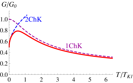
Figure 3: (Color online) Temperature dependence of tunneling conductance (solid curve). Low-$T$ orbital 2CKE and high-T 1CKE spin SO(5) asymptotics are shown by the dashed curves. The input parameters are specified in the text

This equation predicts the crossover from conventional 1CK behavior of tunneling conductance at high temperatures, to NFL criticality characterized by $\sqrt{T}$ behaviorAff05 at low temperatures.

Numerical estimates of the RG parameters using input values of the energy intervals $\Delta_{T_{g},S_{u}}$=0.03, $~{}\Delta_{S_{u},T_{u}}$=0.015, $\Delta_{T_{u},S_{g}}$=0.056 (all in units of $D_{0}$) show that the Haldane RG transformation stops at ${\bar{D}}/D_{0}=0.053$ (the dependence $\bar{D}(\Lambda)$ is neglected in this estimate). As is known KA01 ; KKA04 , the Kondo temperature for CQD displaying $SO(n)$ symmetry is non-universal and depends on the width of the corresponding multiplet. In our estimate $T_{K1}(\Delta_{\rm SO(5)})$= 0.0054$D_{0}$. On the other hand, the two-channel Kondo temperature $T_{K1}$ found from Eqs. (12) without 3-rd order terms on the RHS is $T_{K2}$=0.018$D_{0}\gg T_{K1}$. The reasons for such strong enhancement are (i) the inequality $T_{K1}(\Delta_{\rm SO(5)})\ll T_{K1}(0)$ KKA04 , (ii) the contribution of the enhanced parameter $\bar{j}_{2}$ to the first two equations in the system (12): in accordance with our numerical calculations $\bar{j}_{2}/j_{2}\approx 1.5$, hence $T^{*}/T_{K1}\gg 1$.

This result may be compared with the situation arising in doubly occupied DQD in the serial geometry without source - drain symmetry, where the difference between the high-energy and low-energy scales is related to the crossover from single channel KE to 2CKE due to asymmetry between the source/dot and drain/dot coupling.Logan The crossover mechanism 1CKE$\to$ 2CKE is different in that case (two-stage Kondo screening of two spins ${\bf S}_{(s,d)}$ attached to two electrodes with essentially differing Kondo scales ${T}_{Ks}\gg{T}_{Kd}$ Zar06 ). The 1CKE is characterized by the scale ${T}_{Ks}$, and the 2CKE regime arises at essentially lower temperature $T_{2K}\ll{T}_{Ks}$ due to overscreening of the remaining spin 1/2 by the remaining electrons in the source and drain leads. Comparing the two mechanisms, we see that unlike Ref. Logan, , our mechanism leads to enhancement of the Kondo scale in the crossover 1CKE $\to$ 2CKE.

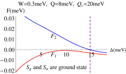
Figure 4: (Color online) Functions $F_{1}(\Delta)$ and $F_{1}(\Delta)$ defining the width of a window for orbital 2CKE [see text below and Eq. (C) for more details.]

Experimentally, the mutual disposition of singlet and triplet levels $E_{\Lambda}$ (3) should be tunable by varying the gate voltages which control the dot parameters such as $\Delta$, $Q_{c}$ and $Q$ in order to drive a TQD into the window defined by inequalities (C). Since these parameters enter the corresponding equations in many ways, it is difficult to point out their optimum combination. Figure 4 shows that the ground state of TQD is formed by two singlets in a wide enough range of the values of parameter $\Delta$ (marked by a vertical dashed line) at realistic values of other model parameters.

IV Concluding remarks

We demonstrate in this paper that the transformation of the conventional high-temperature 1-channel spin-Kondo effect into unconventional low-temperature 2-channel orbital Kondo effect, where spin enumerates the screening channels, is possible in doubly occupied parallel TQD. The mechanism of this transformation is related to the singlet-triplet level crossing (Fig. 2). The necessary precondition for such crossover is the presence of at least two spin singlets in the low-energy spectrum of CQD. In case of TQD with $N=2$ the low-energy spectrum is formed by $SO(8)$ two-triplets/two singlets multiplet. The minimal dynamical symmetry group possessing the demanded properties is $SO(5)$. The theory is developed for the latter case, but the generalization for higher $n$ is straightforward.

Specific feature of dynamical symmetry which is crucial for 1CK $\to$ 2CK crossover is dependence of this type of symmetry on the actual energy scale. It seen from the phase diagram of Fig. 2 that in the ultraviolet high-energy limit $SO(5)$ dynamical symmetry is realized when the highest triplet $T_{g}]$ is integrated out. The ground state in this limit is singlet, so only the usual Kondo scattering in the weak-coupling regime due to singlet/triplet excitations is possible. Dramatic change of Kondo mechanism occurs because in the low-energy limit the ground state becomes quasi doubly degenerate due to $S_{u}/T_{u}$ level crossing. Then the roles of spin and charge degrees of freedom in Kondo scattering swaps, and 2CK effect is realized in a strong-coupling limit. Thus the dynamical symmetry crossover $SO(5)\to SU(2)$ is not simple reduction of the number of relevant degrees of freedom but reconstruction of the ground state in the course of scaling renormalization.

Remarkable feature of this mechanism is the effect of enhancement of the 2CK Kondo temperature in comparison with that for 1CK regime. This effect is robust because the former ”inherits” the Kondo cloud from the latter. Enhancement of Kondo temperature accompanying symmetry reduction $SO(5)\to SU(2)$ contrasts with the general trend of reduction of $T_{K}$ with decreasing number of relevant degrees of freedom, known, e.g. for the $SU(4)\to SU(2)$ crossover.Eto05 ; Lim06 ; Roura11

Several remarks about experimental aspects of the predicted phenomenon are in order. We have already mentioned that the most promising device for realization of the proposed 2CKE regime within the present scenario is an axially symmetric vertical TQD.Amaha09 This technology allows one to fabricate symmetric or at least nearly symmetric isosceles TQD. A Small deviation from the perfect isosceles geometry is not detrimental for observation of the orbital 2CKE. The main effect of violating the left-right symmetry is expressed by the inequality $\varepsilon_{l}\neq\varepsilon_{r}$. Inserting the corresponding corrections into Eqs. (3), we find that this deviation causes additional shifts of the levels $E_{S_{u}}$ and $E_{S_{g}}$, that eventually implies the increment of the effective ”magnetic field” $K_{h}$ in the Hamiltonian $H_{\rm orb}$ (10). Since magnetic field is a relevant parameter for NFL criticality,Aff05 this increase does not prevent observation of 2CKE as soon as the inequalities (C) are valid. In particular, the field dependence of conductance $[G(T,K_{h})-G(T,0)]/G_{0}$ is given by a complicated scaling function derived in Ref. PuBord04, . The quantum critical point 2CKE-1CKE may also be achieved using the mutual disposition of the pairs $E_{T_{u,g}}$ and $E_{S_{u,g}}$ (Fig. 2) governed by the Coulomb blockade energies as control parameters. With reasonable effort, the experimental techniques reported in Ref. Amaha09, can be modified and employed to test the present prediction.  
Acknowledgement This research is partially supported by ISF grants 173/2008 and 400/12.

Appendix A Eigenstates of doubly occupied symmetric TQD

The Hamiltonian of the isolated isosceles TQD is:

$$H_{d}=\sum_{a=l,r,c}\sum_{\sigma}\varepsilon_{a}d^{\dagger}_{a\sigma}d_{a\sigma}$$

$$+\sum_{a}Q_{a}n_{a\uparrow}n_{a\downarrow}+\sum_{i=l,r}Q_{ic}n_{i\uparrow}n_{c\downarrow}$$

$$+W\sum_{i\sigma}(d^{\dagger}_{c\sigma}d_{i\sigma}+H.c.).$$ (22)

Here $\varepsilon_{a}$ are the energy level positions in the central $(c)$ and side $(l,r)$ wells of TQD, $Q_{a}$ and $Q_{ic}$ are intradot and interdot Coulomb blockade parameters, respectively, $W$ is the tunneling integral between the central and side wells. We will be interested in the completely symmetric case, $\varepsilon_{l}=\varepsilon_{r}\equiv\varepsilon,$ $Q_{l}=Q_{r}\equiv Q\ll Q_{c}$ and $Q_{lc}=Q_{rc}\equiv Q_{ic}$.

The Hamiltonian (22) can be diagonalized by using the basis of two–electron wave functions

$$|s_{i}\rangle=\frac{1}{\sqrt{2}}\left(d^{+}_{i\uparrow}d^{+}_{c\downarrow}-d^{+}_{i\downarrow}d^{+}_{c\uparrow}\right)|0\rangle,$$

$$|t_{i},1\rangle=d^{+}_{i\uparrow}d^{+}_{c\uparrow}|0\rangle,$$

$$|t_{i},0\rangle=\frac{1}{\sqrt{2}}\left(d^{+}_{i\uparrow}d^{+}_{c\downarrow}+d^{+}_{i\downarrow}d^{+}_{c\uparrow}\right)|0\rangle,$$

$$|t_{i},\bar{1}\rangle=d^{+}_{i\downarrow}d^{+}_{c\downarrow}|0\rangle,$$

$$|{ex}_{i}\rangle=d^{+}_{i\uparrow}d^{+}_{i\downarrow}|0\rangle,\ \ \ |{ex}_{c}\rangle=d^{+}_{c\uparrow}d^{+}_{c\downarrow}|0\rangle,$$

$$|{ex}_{lr}\rangle=\frac{1}{\sqrt{2}}\left(d^{+}_{l\uparrow}d^{+}_{r\downarrow}-d^{+}_{l\downarrow}d^{+}_{r\uparrow}\right)|0\rangle,$$

$$|{ex}_{lr}^{t},1\rangle=d^{+}_{l\uparrow}d^{+}_{r\uparrow}|0\rangle,$$

$$|{ex}_{lr}^{t},0\rangle=\frac{1}{\sqrt{2}}\left(d^{+}_{l\uparrow}d^{+}_{r\downarrow}+d^{+}_{l\downarrow}d^{+}_{r\uparrow}\right)|0\rangle,$$

$$|{ex}_{lr}^{t},\bar{1}\rangle=d^{+}_{l\downarrow}d^{+}_{r\downarrow}|0\rangle.$$ (23)

In this basis, the Hamiltonian (22) is decomposed into triplet and singlet matrices,

$$H_{t} = \left(\begin{array}[]{ccc}\tilde{\varepsilon}&0&W\\ 0&\tilde{\varepsilon}&-W\\ W&-W&2\varepsilon\\ \end{array}\right),$$ (27)

$$H_{s} = \left(\begin{array}[]{cccccc}\tilde{\varepsilon}&0&W&\sqrt{2}W&0&\sqrt{2}W\\ 0&\tilde{\varepsilon}&W&0&\sqrt{2}W&\sqrt{2}W\\ W&W&2\varepsilon&0&0&0\\ \sqrt{2}W&0&0&2\varepsilon+Q&0&0\\ 0&\sqrt{2}W&0&0&2\varepsilon+Q&0\\ \sqrt{2}W&\sqrt{2}W&0&0&0&2\varepsilon_{c}+Q_{c}\\ \end{array}\right),$$ (34)

where $\tilde{\varepsilon}={\varepsilon}_{c}+\varepsilon+Q_{ic}$.

The low-energy multiplet of two-electron states found by means of diagonalization of the matrices (27) is given by Eqs. (3). The eigenfunctions corresponding to the energies (3) are

$$|S_{g}\rangle = \alpha_{g}\frac{\left|s_{l}\right\rangle+\left|s_{r}\right\rangle}{\sqrt{2}}-\beta_{1}|{ex}_{lr}\rangle$$

$$- \beta_{2}\frac{\left|{ex}_{l}\right\rangle+\left|{ex}_{r}\right\rangle}{\sqrt{2}}-\beta_{3}|{ex}_{c}\rangle,$$

$$|T_{u}\rangle = \alpha^{T}~{}\frac{\left|t_{l}\right\rangle\ -\left|t_{r}\right\rangle}{\sqrt{2}}-\beta_{1}|{ex}^{T}_{lr}\rangle,$$

$$|S_{u}\rangle = \alpha_{u}\frac{\left|s_{l}\right\rangle-\left|s_{r}\right\rangle}{\sqrt{2}}-\beta_{2}\frac{\left|{ex}_{l}\right\rangle-\left|{ex}_{r}\right\rangle}{\sqrt{2}},$$ (35)

$$|T_{g}\rangle = \frac{\left|t_{l}\right\rangle+\left|t_{r}\right\rangle}{\sqrt{2}},$$

where

$$\beta_{1} = \sqrt{2}W/\Delta,~{}\beta_{2}=\sqrt{2}W/(\Delta+Q),$$

$$\beta_{3} = \sqrt{2}W/(\varepsilon_{c}+Q_{c}-Q_{ic}-\varepsilon),$$

$$\alpha_{g} = \sqrt{1-\beta_{1}^{2}-\beta_{2}^{2}-\beta_{3}^{2}},$$

$$\alpha^{T} = \sqrt{1-\beta_{1}^{2}},~{}\alpha_{u}=\sqrt{1-\beta_{2}^{2}}.$$ (36)

Thus the lowest state of the isolated TQD is $E_{S_{g}}$. It is seen from (3) that the singlet and triplet states alternate: $E_{S_{g}}<E_{T_{u}}<E_{S_{u}}<E_{T_{g}}$. The effective RG procedure renormalizing the eigenvalues of quantum dot once it is attached the leads Hald78 , has been generalized for multilevel TQD in Ref. KKA04, In accordance with this procedure, the levels $E_{\Lambda}$ move downward as a function of the scaling parameter $\eta$=$\ln(D/D_{0})$ with different slopes $\varpropto\Gamma_{\Lambda}$. The tunneling rates $\Gamma_{\Lambda}$ for even and odd states (35) obey the following hierarchy: $\Gamma_{T_{g}}>\Gamma_{S_{u}}>\Gamma_{T_{u}}>\Gamma_{S_{g}}$. This means that multiple level crossing is possible in the course of RG evolution. Besides, the pairs $E_{T_{u,g}}$ and $E_{S_{u,g}}$ are subject to level repulsion provided the left and right tunneling channels are not completely independent.

The flow evolution of each level stops at $E_{\Lambda}\approx\bar{D}$. The value $\bar{D}$ is specific for each of the four levels. At this point the SW transformation leads to the Kondo Hamiltonian, and the Kondo-stage of RG procedure starts in accordance with the poor man scaling procedure.And70 The phase diagram is quite complicated, because the two singlet and two triplet levels can intersect in several ways depending on the values of the model parameters $W,\tilde{\varepsilon},\Delta,Q,Q_{c},Q_{ic}$. Among these scenarios are: (I) S=1 Kondo regime corresponding to the scenario where $T_{g}$ is the ground state, and the flow pattern of dynamical symmetries with the RG procedure is $SO(8)\to SO(5)\to SO(4)\to SO(3)$ (cf. the case of TQD with $N=4$ studied in Ref. KKA04, ); (II) Absence of KE corresponding to the scenario where $S_{g}$ is the ground state; (III) Orbital KE with almost degenerate $S_{g},S_{u}$ ground state. Here we focus on two competing phases, namely $SO(5)$ configuration, which involves two singlet states and one triplet state, and orbital $SU(2)$ configuration, where two singlets form (quasi) degenerate pair and the triplet state is involved as a relatively soft excitation above this doublet.

Appendix B $SO(5)$-symmetry

The effective Hamiltonians acting in the Fock space $T_{u},S_{g},S_{u}$ possess the $SO(5)$ symmetry. Ten group generators of the $o_{5}$ algebra can be combined, in particular in three vectors and one scalar.Dynsym In our case these are the vectors ${\bf S}_{u},{\bf R}_{u}$ and the the vector intermixing $g$- and $u$-states, namely, ${\bf\tilde{R}}={\bf{R}}^{(1)}_{ug}+{\bf{R}}^{(2)}_{gu}$ (III). All these operators are defined via Hubbard operators connecting different states of the octet,

$$S^{+}_{u} = \sqrt{2}(X^{1_{u}0_{u}}+X^{0_{u}\bar{1}_{u}}),\ S^{-}_{u}=(S^{+}_{u})^{\dagger},$$

$$S^{z}_{u} = X^{1_{u}1_{u}}-X^{\bar{1}_{u}\bar{1}_{u}},$$

$$R^{+}_{u} = \sqrt{2}(X^{1_{u}S_{u}}-X^{S_{u}\bar{1}_{u}}),\ R^{-}_{u}=(R^{+}_{u})^{\dagger},$$

$$R^{z}_{u} = -(X^{0_{u}S_{u}}+X^{S_{u}0_{u}}),$$ (37)

$$R^{(1)+}_{ug} = \sqrt{2}X^{1_{u}{S}_{g}},\ \ \ {R}^{(1)-}_{ug}=(R^{(1)+}_{ug})^{{\dagger}},$$

$$R^{(1)z}_{ug} = -X^{0_{u}S_{g}},$$

$$R^{(2)+}_{gu} = -\sqrt{2}X^{S_{g}{\bar{1}}_{u}},\ \ \ \ {R}^{(2)-}_{gu}=(R^{(2)+}_{gu})^{{\dagger}},$$

$$R^{(2)z}_{gu} = -X^{S_{g}0_{u}}.$$

and the scalar operators $A$ interchanging $g,u$ variables of the degenerate singlets:

$$A = i(X^{S_{u}S_{g}}-X^{S_{g}S_{u}}).$$ (38)

The exchange part of the effective $SO(5)$ Hamiltonian Hamiltonian arising as a result of two-stage Haldane-Anderson scaling procedureHald78 ; And70 has the form

$$H_{spin} = J_{1}{\bf S}_{u}\cdot{\bf s}_{u}+J_{2}{\bf R}_{u}\cdot{\bf s}_{u}+J_{3}({\bf R}^{(1)}_{ug}\cdot{\bf s}_{gu}+{\bf R}^{(2)}_{gu}\cdot{\bf s}_{ug})$$ (39)

$$+ J_{4}{\bf S}_{u}\cdot{\bf s}_{g}+J_{5}{\bf\tilde{R}}\cdot{\bf s}_{u}$$

$$+ J_{6}({\bf R}_{1g}\cdot{\bf s}_{ug}+{\bf R}_{2g}\cdot{\bf s}_{gu})+J_{7}{\bf S}_{u}\cdot({\bf s}_{gu}+{\bf s}_{ug})$$

$$+ J_{8}({\bf R}^{(1)}_{ug}\cdot{\bf s}_{ug}+{\bf R}^{(2)}_{gu}\cdot{\bf s}_{gu})$$

$$+ J_{9}{\bf R}_{u}\cdot{\bf s}_{g}+J_{10}{\bf\tilde{R}}\cdot{\bf s}_{g}+J_{11}{\bf R}_{u}\cdot({\bf s}_{gu}+{\bf s}_{ug})$$

$$+ J_{12}({\bf R}_{1g}\cdot{\bf s}_{gu}+{\bf R}_{2g}\cdot{\bf s}_{ug}),$$

where

$${R}^{+}_{1g} = -\sqrt{2}X^{S_{g}\bar{1}_{g}},\ \ \ \ {R}^{-}_{1g}=\sqrt{2}X^{S_{g}1_{g}},\ \ \ \ {R}_{1gz}=-X^{S_{g}0_{g}},$$

$${R}^{+}_{2} = (\tilde{R}^{-}_{1})^{\dagger},\ \ \ \ \ \ \ \ \ \;{R}^{-}_{2}=(\tilde{R}^{+}_{1})^{\dagger},\ \ \ \ \ \ \ \ {R}_{2z}=\tilde{R}_{1z}^{\dagger}.$$ (40)

The spin operators for the electrons in the leads are introduced by the obvious relations

$${\bf s}_{g}=\frac{1}{2}\sum_{kk^{\prime}}\sum_{\sigma\sigma^{\prime}}c^{\dagger}_{gk\sigma}\hat{\tau}_{\sigma\sigma^{\prime}}c_{gk^{\prime}\sigma^{\prime}},$$

$${\bf s}_{u}=\frac{1}{2}\sum_{kk^{\prime}}\sum_{\sigma\sigma^{\prime}}c^{\dagger}_{uk\sigma}\hat{\tau}_{\sigma\sigma^{\prime}}c_{uk^{\prime}\sigma^{\prime}},$$

$${\bf s}_{gu}=\frac{1}{2}\sum_{kk^{\prime}}\sum_{\sigma\sigma^{\prime}}c^{\dagger}_{gk\sigma}\hat{\tau}_{\sigma\sigma^{\prime}}c_{uk^{\prime}\sigma^{\prime}},\ \ {\bf s}_{ug}=({\bf s}_{gu})^{{\dagger}}.$$ (41)

Here the first three effective exchange constants are

$$J_{1}(\varepsilon)=\frac{\alpha_{T}^{2}V^{2}}{\varepsilon_{F}-\varepsilon},\ \ \ \ \ \ \ \ J_{2}(\varepsilon)=-\frac{\alpha_{u}\alpha_{T}V^{2}}{\varepsilon_{F}-\varepsilon},$$ (42)

$$J_{3}(\varepsilon)=-\frac{\alpha_{g}\alpha_{T}V^{2}}{\varepsilon_{F}-\varepsilon},$$

and the rest coupling parameters arise at the second stage of RG procedure, which starts with the initial conditions

$$J_{1}(\bar{D})=J_{1},\ \ \ \ \ \ \ J_{2}(\bar{D})=J_{2},$$

$$J_{3}(\bar{D})=J_{3},\ \ \ \ \ J_{i}(\bar{D})=0~{}~{}~{}~{}(i=4-12)$$ (43)

The RG flow equations for these 12 coupling constants are derived in Ref. KKA04, . Analysis of these equations shows that only three first vertices (42) are relevant, and one may use the reduced Hamiltonian (6) for calculation of the fixed point solution, which corresponds to the Kondo temperature

$$T_{K2}=\bar{D}\Big{(}1-\frac{2\sqrt{2}m_{lr}}{j_{1}+j_{2}+\sqrt{(j_{1}+j_{2})^{2}+2j_{3}^{2}}}\Big{)}^{\displaystyle{\frac{1}{\sqrt{2}m_{lr}}}}$$ (44)

where $j_{i}=\rho_{0}J_{i}$ ($i=1,...,12$), $d=\rho_{0}D$ and $m_{lr}=\rho_{0}\bar{M}_{lr}.$ This expression transforms to Eq. (9) at $m_{lr}\to 0$.

Appendix C Orbital KE

The singlets $S_{g}$ and $S_{u}$ become the lowest renormalized states in the SW limit, i.e., $\bar{E}_{S_{g}}=\bar{E}_{S_{u}}-2{K}_{h}<\bar{E}_{T_{g}},\bar{E}_{T_{u}}$, when

$$F_{1}<0,~{}~{}~{}F_{2}>0,$$

(45)

$$F_{1}=\frac{2W^{2}\beta_{2}^{2}}{\beta_{1}^{2}+\beta_{3}^{2}}\left(\frac{1}{\Delta}+\frac{2}{\varepsilon_{c}+Q_{c}-Q_{ic}-\varepsilon}\right)-$$

$$\frac{2W^{2}}{\Delta+Q}+{K}_{h},$$

$$F_{2}=\frac{2W^{2}Q}{\Delta(\Delta+Q)}-$$

$$\frac{2W^{2}(\beta_{1}^{2}-\beta_{2}^{2})}{\beta_{1}^{2}+\beta_{3}^{2}}\left(\frac{1}{\Delta}+\frac{2}{\varepsilon_{c}+Q_{c}-Q_{ic}-\varepsilon}\right)-{K}_{h}.$$

Here $K_{h}/2=\bar{M}_{lr}$ is the indirect tunneling amplitude between the side dots via the central dot and the leads arising in the course of renormalizationKKA04 [see also Eq. (C) below].

In this case the two-channel orbital Kondo effect can be realized. The corresponding cotunneling Hamiltonian has the form:

$$H_{\mathrm{orb}}={\bar{M}_{lr}}(X^{uu}-X^{gg})$$

$$+\frac{\alpha_{g}^{2}}{2}\frac{V^{2}}{\varepsilon_{F}-\varepsilon}\sum_{kk^{\prime}\sigma}X^{S_{g}S_{g}}c^{\dagger}_{e,k\sigma}c_{e,k^{\prime}\sigma}$$

$$+\frac{\alpha_{u}^{2}}{2}\frac{V^{2}}{\varepsilon_{F}-\varepsilon}\sum_{kk^{\prime}\sigma}X^{S_{u}S_{u}}c^{\dagger}_{o,k\sigma}c_{o,k^{\prime}\sigma}$$ (46)

$$+\frac{\alpha_{g}\alpha_{u}}{2}\frac{V^{2}}{\varepsilon_{F}-\varepsilon}\sum_{kk^{\prime}\sigma}(X^{S_{g}S_{u}}c^{\dagger}_{o,k\sigma}c_{e,k^{\prime}\sigma}+X^{S_{u}S_{g}}c^{\dagger}_{e,k\sigma}c_{o,k^{\prime}\sigma}),$$

with $c_{(e,o),k\sigma}=\frac{1}{\sqrt{2}}\left(c_{l,k\sigma}\pm c_{r,k\sigma}\right)$, and avoided crossing of the singlet states taken into account. The Hamiltonian (46) can be rewritten in terms of pseudospin Pauli matrices $\vec{\cal{T}}$ and $\vec{\tau}$. It acquires a form given by Eq. (10) with following coupling constants:

$$K_{h} = 2{\bar{M}_{lr}},$$

$$K_{\|} = \frac{\alpha_{g}^{2}+\alpha_{u}^{2}}{2}\frac{V^{2}}{\varepsilon_{F}-\varepsilon},$$

$$K_{\bot} = \frac{\alpha_{g}\alpha_{u}V^{2}}{\varepsilon_{F}-\varepsilon},$$

$$K_{1} = K_{2}=\frac{\alpha_{g}^{2}-\alpha_{u}^{2}}{4}\frac{V^{2}}{\varepsilon_{F}-\varepsilon}.$$ (47)

The anisotropic Hamiltonian (10) describes two-channel orbital Kondo effect in an effective ”magnetic field” $K_{h}$. The coupling constant $K_{h}$ remains unrenormalized (because all the terms $\sim\tau_{z}^{2}$ contribute to $K_{1}$), but it affects the renormalization of the other coupling constants. The scaling equations have the form (12).

References

• (1) P. NoziΓ¨res and A. Blandin, J. Physique 41, 193 (1980).
• (2) W. Hofstetter and G. Zarand, Phys. Rev. B 69, 2353 (2002)
• (3) M. Eto, J. Phys. Soc. Jpn, 74, 95 (2005).
• (4) J.S. Lim, M.-S. Choi, M.Y. Choi, R. Lopez, and R. Aguado, Phys. Rev. B 74, 205119 (2006)
• (5) P. Trocha, Phys. Rev. B 82, 125323 (2010).
• (6) G.C. Tettamanzi, J. Verduijn, G.P. Lansbergen, M. Blaauboer, M.J. CalderΓ³n, R. Aguado, S. Rogge, Phys. Rev. Lett. 108, 046803 (2012)
• (7) R.M. Potok, I.G. Rau, H. Shtrikman, Y. Oreg, and D. Goldhaber-Gordon, Nature 446, 167 (2007).
• (8) T. Kuzmenko, K. Kikoin, and Y. Avishai, Europhys. Lett. 64, 218 (2003).
• (9) J. Kondo, Physica 84B, 40, 207 (1976).
• (10) K. VladΓ‘r, A. Zawadowski, Phys. Rev. B bf 28, 1564, 1582 (1983).
• (11) A.L. Moustakas and D.S. Fisher, Phys. Rev. 53, 6832 (1996).
• (12) A.L. Moustakas and D.S. Fisher, Phys. Rev. 55, 4300 (1996).
• (13) D.L. Cox and A. Zawadowski, Adv. Phys. 47, 943 (1998).
• (14) Yu.M. Kagan and N.V. Prokof’ev, Sov. Phys. JETP 63, 1276 (1986); 69, 836 (1989).
• (15) I.L. Aleiner, B.L. Altshuler, Y.M. Galperin, and T.A. Shutenko, Phys. Rev. Lett. 86, 2629 (2001).
• (16) I.L. Aleiner and D. Controzzi, Phys. Rev. B 66, 045107 (2002).
• (17) G. Zarand, Phys. Rev. B 72, 245103 (2005).
• (18) T. Cichorek, A. Sanchez, P. Gegenwart, F. Weickert, A. Wojakowski, Z. Henkie, G. Auffermann, S. Paschen, R. Kniep, and F. Steglich, Phys.Rev. Lett. (2005)
• (19) J. von Delft, A.W.W. Ludwig, and V. Ambegaokar, Ann. Phys. 273, 175 (1999).
• (20) K.A. Matveev, Phys. Rev. B 51, 1743 (1995).
• (21) E. Lebanon, A. Schiller, Phys. Rev. B 64, 245338 (2001).
• (22) M. Arnold, T. Langenbruch, and J. Kroha, Phys. Rev. Lett. 99, 186601 (2007).
• (23) K.T. Law, C.Y. Seng, P.A. Lee, and T.K. Ng, Phys. Rev. B 81, 041305 (2010).
• (24) S. Amaha, T. Hatano, S. Teraoka, A. Shibatomi, S. Tarucha, Y. Nakata, T. Miyazawa, T. Oshima, T. Usuki, and N. Yokoyama, Appl. Phys. Lett. 92, 202109 (2008); A.S. Amaha, T. Hatano, T. Kubo, S. Teraoka, Y. Tokura, S. Tarucha, and D.G. Austing, Ibid. 94, 092103 (2009).
• (25) K. Kikoin, M.N. Kiselev and Y. Avishai, Dynamical Symmetries for Nanostructures, Springer, Wien 2012.
• (26) K. Kikoin and Y. Avishai, Phys. Rev. Lett. 86, 2090 (2001); Phys. Rev. B 65, 115329 (2002).
• (27) T. Kuzmenko, K. Kikoin, and Y. Avishai, Phys. Rev. Lett. 89, 156602 (2002); Phys. Rev. B 69, 195109 (2004).
• (28) F. D. M. Haldane, Phys. Rev. Lett. 40, 416 (1978).
• (29) The singlet-triplet level crossing was discussed in Ref. MuFi97, for a heavy impurity with four electrons captured in a three-well trap with triangular symmetry $C_{3v}$ in the presence of the Jahn-Teller effect.
• (30) P.W. Anderson, J. Phys. C 3, 2435 (1970).
• (31) I. Affleck, J. Phys. Soc. Jpn. 74, 59 (2005); Lecture Notes, Les Houches Summer School 89, pp. 3-64 (2008).
• (32) C. A. BΓΌsser, E. Vernek, P. Orellana, G.A. Lara, E.H. Kim, A.E. Feiguin, E.V. Anda, and G.B. Martins, Phys, Rev. B bf83, 125404 (2011)
• (33) A.K. Mitchell, E. Sela, and D.E. Logan, Phys. Rev. Lett. 108, 086405 (2012).
• (34) G. Zarand, C.-H. Chung, P. Simon, and M. Vojta, Phys. Rev. Lett. 97, 166802 (2006).
• (35) P. Roura-Bas, L. Tosi, A.A. Aligia, and K. Hallberg, Phys. Rev. B 84, 073406 (2011).
• (36) M. Pustilnik, L. Borda, L.I. Glazman,and J. von Delft, Phys. Rev. B 69, 115316 (2004).