A search for radio pulsars and fast transients in M31 using the WSRT

Abstract

We present the results of the most sensitive and comprehensive survey yet undertaken for radio pulsars and fast transients in the Andromeda galaxy (M31) and its satellites, using the Westerbork Synthesis Radio Telescope (WSRT) at a central frequency of 328 MHz. We used the WSRT in a special configuration called 8gr8 (eight–grate) mode, which provides a large instantaneous field-of-view, about 5 square degrees per pointing, with good sensitivity, long dwell times (up to 8 hours per pointing), and good spatial resolution (a few arc minutes) for locating sources. We have searched for both periodicities and single pulses in our data, aiming to detect bright, persistent radio pulsars and rotating radio transients (RRATs) of either Galactic or extragalactic origin. Our searches did not reveal any confirmed periodic signals or bright single bursts from (potentially) cosmological distances. However, we do report the detection of several single pulse events, some repeating at the same dispersion measure, which could potentially originate from neutron stars in M31. One in particular was seen multiple times, including a burst of six pulses in 2000 seconds, at a dispersion measure of 54.7 pc cm^-3, which potentially places the origin of this source outside of our Galaxy. Our results are compared to a range of hypothetical populations of pulsars and RRATs in M31 and allow us to constrain the luminosity function of pulsars in M31. They also show that, unless the pulsar population in M31 is much dimmer than in our Galaxy, there is no need to invoke any violation of the inverse square law of the distance for pulsar fluxes.

1 Introduction

Extragalactic radio pulsars, i.e. pulsars located in galaxies beyond our own Galaxy and its satellites, have yet to be detected. This is primarily because they are at least 100 times more distant than the majority of the known population of radio pulsars in our Galaxy. To date, the most distant pulsars detected have been found inside the Large Magellanic Cloud (LMC) and the Small Magellanic Cloud (SMC), located at distances of 49 and 57 kpc respectively (e.g. Manchester et al. 2006). Several attempts to detect extragalactic radio pulsars have been made in the past. Linscott & Erkes (1980) reported the detection of highly dispersed radio pulses from M87 with a duration of 50 ms. These findings however were not confirmed by Hankins et al. (1981), McCulloch et al. (1981) or Taylor et al. (1981).

The brightest radio bursts known are the giant pulses seen from the Crab pulsar (Cordes et al. 2004) and a handful of other neutron stars. These pulses are very narrow (in some cases with structure still unresolved at 2-ns time resolution) and very bright ($>10^{5}$ Jy) as reported by Hankins et al. (2003). Due to their brightness, giant pulses may in principle be detected in other galaxies and McLaughlin & Cordes (2003) performed searches for giant pulses from M33, the LMC, NGC253, NGC300, Fornax, NGC6300 and NGC7793, but with no confirmed detections. More recently, Bhat et al. (2011) undertook a search for pulsars in M33 at 1400 MHz, also with null results.

Generally, pulsar surveys use two complementary search techniques: Fourier-based periodicity searches as well as searches for dispersed single pulses. Periodicity searches are poorly optimized for sources that exhibit pulses with a wide range of intensities, as comprehensively discussed by Cordes & McLaughlin (2003). Single pulse searches can be more powerful than periodicity searches if the source emits bright but rare pulses and/or shows a shallow power-law pulse energy distribution. In these searches, individual bright, dispersed pulses are recorded and subsequently analyzed to establish a possible underlying periodicity, which does not necessarily show up in a periodicity search.

In recent years, single pulse search methods have become standard practice and are now employed in most of the on-going pulsar surveys. This has resulted in two important discoveries. The first is the population of rotating radio transients (RRATs, McLaughlin et al. 2006), objects which are characterized by their sporadic, bright radio pulses, and which possibly represent a subset of the total radio pulsar population. McLaughlin et al. (2006) show that RRATs are among the most luminous radio sources known when they emit ($L_{1400}\sim$ 1–3.6 Jy kpc²), though they are still weaker than the giant pulses seen from, e.g., the Crab pulsar and PSR B1937+21. RRATs can account for a considerable fraction of the active radio-emitting neutron stars in our Galaxy and their high luminosity may make it possible to detect them in nearby galaxies. The second discovery is the detection of what appears to be a single radio pulse of extragalactic origin: the “Lorimer Burst” (Lorimer et al. 2007), an extremely bright ($S_{1400}\sim 30$ Jy), $\sim 5$-ms-wide pulse from a high Galactic latitude and with a high dispersion measure (hereafter DM) of about $375$ pc cm^-3, both which suggest an origin well beyond our galaxy ($d\geq$ 1 Gpc). Such a burst could, e.g., be associated with the coalescence of two neutron stars (Hansen & Lyutikov 2001) or the evaporation of a black hole (Rees 1977). Other detections of this kind (Keane et al. 2011) with other observatories and, especially, where the source position can be better localized, would help to elucidate the true nature of this phenomenon.

Searching for extragalactic pulsars is motivated by gaining a better understanding of galactic pulsar populations, especially when the star formation rate and stellar evolution history differ from those in our Galaxy. The sensitivity of current radio telescopes is such that we are in a position to detect only the most luminous pulsars in the nearby galaxies of our Local Group. The direct comparison of a pulsar location with that of the known supernova remnants in M31 such as those found by  Gelfand et al. (2005), would be difficult due to the small angular size of these remnants. However, if the pulsar age is also determined, associations may be possible if the supernova remnants are still bright (Narayan & Schaudt 1988). This correlation can help determine the formation ratio of rotation-powered pulsars versus other manifestations of neutron stars like magnetars, and other compact objects like black holes in nearby galaxies. By measuring the DM of sources in M31 and comparing them with the models of free electrons for our Galaxy, we can estimate limits on the contributions to the DM due to the interstellar medium in M31, assuming that we know the contribution due to our own galaxy, within the limits of accuracy of the NE2001 model of Cordes & Lazio (2002) (the contribution of the intergalactic medium is likely to be negligible). Finally, by measuring the rotation measure (RM) it might also be possible to obtain an estimate of the magnetic field along the line-of-sight to Andromeda.

The detection of pulsars in other Local Group galaxies is challenging, however. In the case of M31, the disk of the galaxy covers a significant area of sky ($190^{\prime}\times 60^{\prime}$) and the distance, $\sim 778$ kpc (Karachentsev et al. 2004), means that any pulsar signal is likely to be extremely faint. An effective search also requires long dwell times in order to catch rare, bright bursts. A deep search of M31 can be achieved by using the WSRT in a special mode called 8gr8, which makes optimal use of the array’s linear configuration, in combination with the Pulsar Machine (PuMa; Voûte et al. 2002) backend. The 8gr8 mode provides a $\sim$2.5-deg-wide field-of-view (FoV), that of the primary beam of the individual 25-m WSRT dishes, as well as the full sensitivity and angular resolution of all the dishes combined in a tied-array. This enables the possibility of locating new sources with good accuracy (a few arcminutes) if the source emits bright periodic pulses or, at least, multiple bright bursts at different hour angles.

In this paper, we present a search of the Andromeda galaxy (M31) and its satellites (M32, M110 and a few other dwarf galaxies). In §2 we describe the observations and the 8gr8 technique; in §3 we present the data analysis and describe the search methodology; in §4 we present the search results; and in §5 we compare our results to our current understanding of the luminosity distributions of pulsars and RRATs in our own Galaxy. Lastly, our conclusions are presented in §6.

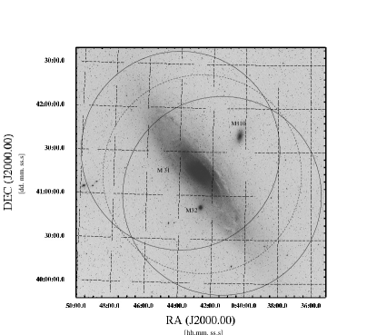
Figure 1: A Sloan Digital Sky Survey image of M31. The circles represent the half power beam width of the individual WSRT dishes at a frequency of 328 MHz, which cover approximately 5 square degrees each. The solid lines represent the two main pointings of this survey, PNT01 (south) and PNT02 (north), while the dotted line represents PNT03, a complementary pointing centered on the core of M31  (see Table 1 for reference). M32 and M110 also fit within the beams (see labels on the figure).

Table 1: WSRT observations of M31. $N_{\rm P}$ is the number of pointings at each position. The start times of the individual pointing are given in Table 7 of Appendix A.

Pointing	R.A.(J2000.0)	DEC.(J2000.0)	$N_{\rm P}$	Dwell
Name	(h.m.s.)	(d.m.s.)		Time (hr)
M31 PNT01	00 41 30	+41 00 00	4	8
M31 PNT02	00 44 00	+41 30 00	4	8
M31 PNT03	00 42 45	+41 15 00	2	8

2 WSRT 8gr8 Observations

We observed two main pointings along the disk of M31 (solid circles of Fig. 1) and later also one complementary pointing centered on the core of the galaxy (dashed circle of Fig. 1). Each of the main pointings was observed for 32 h total, divided in to four 8-h observations, separated by intervals of approximately one day. The complementary pointing was observed for 16 h in two 8-h sessions at a later epoch. We recorded two polarizations (summed in quadrature), each with 10 MHz of bandwidth at a center frequency of 328 MHz. The digital filter-bank PuMa (Voûte et al. 2002) was used to write spectra with 256 frequency channels and $t_{\rm s}=$ 409.6 $\mu$s sampling, producing $2^{26}$ samples per observation. Table 1 summarizes these observations, which were performed in 2005 October using the WSRT in 8gr8 mode (see also Janssen et al. 2009). In this mode, 12 dishes of 25 m in diameter, and equally spaced by 144 m, are used to form an array with the equivalent collecting area of a single 74-m dish.

Figure 2: An example of how sources can be localized using the 8gr8 method. The panels show two examples of beam plots. The upper panel shows the original and confirmation observations in which PSR J1937+2950 was detected using a periodicity search (position shown with a cross, figure taken from Janssen et al. 2009). These observations were each 2 h long and were done at hour angles of HA${}_{1}=138.81^{\circ}$ and HA${}_{2}=201.31^{\circ}$. In the lower plot we show the original and confirmation observations in which single pulses from the known pulsar PSR B1946+35 were detected (position shown with large cross). These observations were done at hour angles HA${}_{1}=174.45^{\circ}$ and HA${}_{2}=244.45^{\circ}$ respectively. In both panels solid dots represent sub-beams in which the pulsar was detected in the first observation while the open circles represent detections made in the confirmation observation. The sizes of all the circles are proportional to the S/N of the detections. In both cases, the two observations at different hour angles allow us to accurately locate the source.

When the signals of the 12 dishes are coherently added, having corrected for instrumental and geometrical phase delays, we obtain an elliptically shaped fan beam. The major axis of the fan beam spans the entire primary beam of the 25-m dishes, and the minor axis is inversely proportional to the separation of the furthest dishes. Due to the regular spacing of the dishes along the East–West axis, they produce a grating response on the sky with parallel fan beams equally spaced across the primary beam and separated by $c/(B\nu)$ radians, where $B$ is the projected baseline between the dishes, $\nu$ is the observing frequency and $c$ is the speed of light. Each such collection of fan beams are referred to as a “grating group” from now on. Since the WSRT has eight independent signal chains, which can each have their own separate phase-tracking center, we can simultaneously form and record eight grating groups on the sky.

These grating groups allow us to almost fully tessellate the entire primary beam. At a later stage, the eight grating groups can be linearly combined in software into $N_{\rm total}$ elliptical sub-beams to cover the entire FoV of the primary beam by making use of the fact that the grating groups rotate relative to the sky during the observation. Each of the sub-beams covers an angular size of approximately $\sim 1.8$ arcmin, at an observing frequency of 328 MHz, and is spaced in such a way so as to overlap with adjacent sub-beams at the half power point. The total number of sub-beams $N_{\rm total}$ varies per observation between 900 and 1100, and depends on the position of the main beam on the sky (hour angle) and the length of the observation. Each sub-beam has a comparable sensitivity to a coherent combination of all 12 dishes. Each of these sub-beams is searched for dispersed, pulsed signals and single bursts. The sub-beams allow us to localize sources with modest precision when we have detections from observations made at different hour angles, since the different orientations of the fan beams allow one to localize the source at the crossing points of these beams. Having a large number of sub-beams also permits us to distinguish spurious detections from real ones because genuine single bursts will be detected in multiple sub-beams.

In the case of periodicity searches, a candidate should appear in multiple detection regions in an observation, as shown in the upper panel of Fig. 2. The number of beams in which the candidate is detected depends on the intensity of the source. For single pulse searches, localization is more complicated because the source will appear in more sub-beams. A genuine astrophysical detection should appear in a number of sub-beams $N_{\rm b}$ such that $N_{\rm max}\geq N_{\rm b}\geq N_{\rm min}$, where $N_{\rm max}\sim 1/8N_{\rm total}$ and $N_{\rm min}\sim 1\%N_{\rm total}$ with the sub-beams making a specific pattern within the primary beam as shown in the lower panel of Fig. 2. Here we show the detection of 8 pulses in total, divided into two groups of 4 pulses, each group from a different observation performed at a significantly different hour angle. A detection appearing in too many sub-beams or too many fan beams ($N_{\rm b}>N_{\rm max}$) is likely to be impulsive radio frequency interference (RFI). In contrast, a detection that appears in too few sub-beams ($N_{\rm b}<N_{\rm min}$) is likely to be a statistical fluctuation.

3 Data reduction

As we describe in detail below, we searched for both periodic and sporadic signals. We first discuss the common elements of the analysis.

The NE2001 model (Cordes & Lazio 2002) predicts a $\mbox{DM}=55\pm 10$ pc cm^-3 for a pulsar at the outer edge of our Galaxy, along the line-of-sight to M31, which lies well out of the Galactic Plane ($b=-21^{\circ}$). To detect sources located well inside M31, we searched a broad range of trial DMs from 0 to 350 pc cm^-3. This DM range covers sources located within our Galaxy ($\mbox{DM}<45$ pc cm^-3), as well as objects that might be located in M31. Our upper limit for the DM trials was set due to the fact that at this high DM the radio pulses are likely severely scattered at 328 MHz. We consider that any value of DM larger than $\sim$ 45 pc cm^-3 may indicate a source location in M31; assuming that the electron distribution in M31 is not too dissimilar to the one in our Galaxy, this DM range would allow us to detect sources reasonably deep into M31, even though it is inclined at only about $13^{\circ}$ to our line-of-sight (Simien et al. 1978). For example, an excess in DM of 10 pc cm^-3 (above that contributed by our Galaxy) would imply a location about 1 kpc inside the outer edge of Andromeda.

Due to the large data volume, each 8-h observation was sub-divided into chunks of 1 h for further processing. For each 1-h chunk, we prepared partially dedispersed time series for each of the 8 grating groups. This was done using a modified version of the tree dedispersion algorithm developed by Taylor (1974), which divides the bandwidth of each fan beam into smaller frequency sub-bands where we assume the dispersive delay to be linear. From these, we form time series for all trial DMs (see below), each consisting of $2^{23}$ samples. Lastly, a geometrical correction was applied before combining the data sets from each of the 8 fan beams into a collection of sub-beams spanning the whole hour.

Each of these sub-beams was searched for periodicities and bright pulses. We searched 549 trial DMs, with step sizes of 0.348, 0.697 and 1.392 pc cm^-3 respectively, each corresponding to the spacing below the first and second “diagonal DM”, located at $\mbox{DM}=83$ and 249 pc cm^-3 respectively. The DM step-sizes were chosen so that the maximum error in the delay between the highest and lowest frequency channels was equal to the sampling time. This search used the PSE code from the Parkes High-Latitude Survey (Edwards et al. 2001), with single-pulse search extensions developed by us (see §3.2).

Figure 3: Diagnostic plot from the single-pulse search, for a single sub-beam and a DM range $0-83$ pc cm^-3. The top panel shows a DM-S/N-time array, with a time resolution of 3.2768 ms, which corresponds to the addition of $2^{3}$ raw samples of 409.6 $\mu$s. The data ends before t=3600 s because we analyzed a timeseries which is the closest power of two number of samples, which for this case is 3436 s long. The sizes of the circles are proportional to the S/N, with the highest S/N $\sim$ 7.9 associated with RFI at low DM. Those detections that matched our RFI filter have been excised from the figure. The second panel from the top shows the time series collapsed along DM in order to more clearly show at which times strong pulses occurred. The lower left panels show two histograms. The top one is the time series collapsed in time, clearly showing a peak at $\mbox{DM}\sim 54\mbox{ pc cm}^{-3}$. The lower one shows a histogram where time is collapsed to show the number of pulses versus DM. The horizontal lines in the bottom left panels show the mean and the 3 and 6-$\sigma$ limits of each distribution. The histogram in the bottom middle part of the figure shows the distribution of pulses with S/N $>5$. The dashed line in this histogram shows the expected noise distribution. This same pointing position was observed for another 31 h without recording the same burst profusion.

3.1 Periodicity search analysis

We performed a periodicity search following the same procedure used by Janssen et al. (2009), but adapted to the specific properties of our data. We calculated the power spectra for each DM trial of each sub-beam using a Fast Fourier Transform (FFT), removing frequencies known to be related to RFI. Interpolation of the spectra was used to recover spectral features lying between Fourier bins (Ransom et al. 2002), repeating the process after summing 2, 4, 8 and 16 harmonics. All the spectral features with a S/N $>$ 7 were recorded, later keeping only the signals that were detected at multiple DMs and appearing to be harmonically related. This was done to find the most significant candidates, and to determine their DM and fundamental frequency. For each candidate, the initial period from the spectral search was optimized by folding the data at a range of periods, assuming a maximum error in the pulse frequency equal to the width of one Fourier bin. No acceleration searches were done. Typically there were a few tens of candidates per sub-beam, i.e. about 30,000 candidates per pointing. Those combinations of DM and spin frequency that produced the highest S/N candidates were stored for later inspection. This process was performed on each of the $N_{\rm total}$ sub-beams. Once this analysis was completed, a list of candidates from the sub-beams was collated and those candidates with high S/N appearing in more than one sub-beam were stored. Later these detections were compared with the lists from the other follow-up pointings, and those candidates that matched with similar periods, DMs and S/N were inspected by eye.

3.2 Single pulse search analysis

We searched for single pulses following two selection criteria: i) single, relatively bright pulses (S/N $>7.0$) or ii) multiple, fainter pulses below this threshold, but repeating at the same DM. We first discuss the general algorithm to search for single pulses, and then discuss the details of the two selection criteria.

As mentioned in §3, for each sub-beam dedispersed time series are generated at all trial DMs. Finding single pulse candidates simply consists of recording those individual events that show an amplitude above some threshold of S/N, which is statistically significant and reduces the number of candidates due to RFI. An extensive description of the method for these searches can be found in Cordes & McLaughlin 2003.

We developed a code to extract individual pulses from each of the time series. We first determine the statistics of the noise in the time series, which each contain $N_{\rm samp}$ samples. This is done by calculating the mean and the rms using an iterative process where the strongest pulses are removed until one reaches the expected number of spurious detections ($N_{\rm noise}$) for a Gaussian distribution with probability $P(x)$, given by $N_{\rm noise}=N_{\rm samp}P(>5\sigma)$, and then searching again for pulses above a 5$\sigma$ threshold. This process keeps the mean and the rms from being biased towards very strong individual pulses. The S/N of a detection in the time series depends on the intrinsic width of the pulse $W$ as S/N $\propto W^{-1/2}$, where the pulses with the highest peak S/N will be those with a width similar to the time resolution of the timeseries. Therefore we explored a range of widths, such that $W_{\rm i}\geq t_{\rm s}$, by adding between 2⁰ and 2⁷ adjacent samples, corresponding to a range in time resolution of 0.4096 – 52.4288 ms. Each of these smoothed time series was then searched for single bright pulses, recording all the pulses that showed a peak S/N $\geq 5$. For each pulse detected we record the DM, the arrival time of the pulse relative to the start of the observation and its S/N. Hereafter we will call this information DM–S/N–time arrays. The S/N threshold was chosen based on the expected number of false detections $N(<$ threshold$)$ above that minimum S/N by assuming that the noise is purely Gaussian. For a time series the number of expected false detections, above a given S/N, can be calculated using a relation shown by Cordes & McLaughlin (2003):

$$N(>\mbox{threshold})\approx 2N_{\mbox{samp}}\int_{\mbox{S/N}_{min}}^{\infty}\exp\left(-x^{2}/2\right)dx.$$ (1)

For a full-resolution, 1-h data set, we expect $N(>5\sigma)\sim$2700 false detections from all the time series required to cover the 549 DM trials.

After searching the dedispersed time series for pulses above the S/N threshold, we created diagnostic plots like the one shown in Fig. 3 to better assess whether any of the signals were astronomical in origin. Such a plot was made for each of the sub-beams. When sorting/inspecting the diagnostic plots, we searched for both i) single bright pulses (S/N $>7.0$) and ii) multiple, weaker pulses recurring at the same DM. As can be seen in Fig 3, the signature of a single bright pulse appears in the top panel of the figure as a large circle (e.g., one can see RFI between $t=500$ and $t=1000$ s), while the signature of multiple weak pulses at the same DM appears as a peak (in this case at $\mbox{DM}=54\mbox{ pc cm}^{-3}$) in either of the two histograms in the lower left area of the plot.

3.3 Single bright pulse search

We recorded all the single pulses with a S/N $>5$ in the DM–S/N–time arrays for each of the smoothed time series, keeping only the information corresponding to those pulses that were detected in a reasonable number of beams ($1/8N_{\rm total}>N_{\rm b}>1\%N_{\rm total}$). For each candidate, we recorded the DM, S/N, time of the event, the number of sub-beams in which the pulse was detected, and in which sub-beam the detection was strongest. We then searched for possible associations, i.e. other pulses occurring at the same DM at later times or in other observations. Those events that had high S/N ($>7.0$) but that did not show any associations were classified as single bright pulses.

3.4 Multiple pulses at the same DM

To search for multiple, potentially weaker events occurring at the same DM we performed a statistical analysis, searching for any excess of S/N in the S/N-DM space. Any excess of S/N due to real pulses would create peaks like those shown in the lower left panels of Figure 3. Detections showing features of this kind, and appearing in a reasonable number of sub-beams ($N_{\rm b}>1\%N_{\rm total}$) were recorded in a list for further inspection. Since there are 900–1100 sub-beams per hour of observation, this produced a very large number of candidates. In order to reduce the number of candidates to inspect, we filtered the list by searching each candidate for “adjacent friends”, i.e. other detections located at adjacent DM trials and occurring at the same time. Cordes & McLaughlin (2003) quantify how the S/N decreases when a pulse is detected at an incorrect DM. Narrow pulses will be detected in few DM bins, therefore will show few adjacent friends, while broader pulses are detected along many DM trials. An example event with adjacent friends is shown in the lower left panels of Fig. 3. This criteria was implemented to estimate the number of adjacent friends a signal of a given DM should have, given the S/N of two adjacent detections. Once the data was filtered in this way, the remaining diagnostic plots were inspected by eye.

3.5 Radio frequency interference excision

To excise RFI from the single-pulse diagnostic plots, we inspected the DM–S/N–time arrays of each of the 8 grating groups. Events aligned in time and appearing along all trial DMs in all 8 data sets were flagged as RFI and recorded in a mask file, in order to excise those time bins when the single pulse analysis was performed.

Figure 4: Minimum detectable flux density for single bright pulses as a function of the number of samples added, assuming a constant peak amplitude, so that sensitivity appears to improve with increasing width. The raw sampling time of our data is $t_{\rm s}=409.6$ $\mu$s and a minimum threshold of S/N=5 was used. Each horizontal line represents the minimum detectable flux for each smoothed time series adding from top to bottom, 2⁰ to 2⁷ samples.

3.6 Sensitivity of WSRT in 8gr8 mode

For periodicity searches, the minimum detectable flux density is given by the modified radiometer equation as follows (Lorimer & Kramer 2005):

$$S_{\rm min}=\beta\frac{\mbox{S/N}_{\rm min}T_{\rm sys}}{G\sqrt{n_{\rm p}t_{\rm d}\Delta f}}\sqrt{\frac{W}{P-W}}.$$ (2)

where $\beta$ is an efficiency factor $\sim 1.3$ related to the 2-bit sampling. S/N_min is the detection threshold, $T_{\rm sys}$ is the system temperature in K ($T_{\rm sky}+T_{\rm receiver}$), $G$ is the gain of the telescope (in K Jy^-1), $n_{\rm p}$ is the number of polarizations, $\Delta f$ is the bandwidth, $P$ is the pulsar period and $W$ is the intrinsic width of the pulse. Using $T_{\rm sys}/G=140$ Jy, $\Delta f=10$ MHz, $n_{\rm p}=2$, a dwell time of $t_{\rm d}=$3600 s, and assuming a mean duty cycle of 5%, we can reach a minimum flux density of $\sim$0.25 mJy for a S/N=7 detection.

Similarly, for the single pulse searches, our sensitivity is given by the radiometer equation, assuming matched filtering to a pulse that is temporally resolved, as follows (Cordes & McLaughlin 2003):

$$S_{\rm min}=\frac{\mbox{S/N}_{\rm min}T_{\rm sys}}{G\sqrt{n_{\rm p}\Delta fW}}.$$ (3)

The minimum detectable flux density depends on the pulse width as $W^{-1/2}$, assuming a constant peak amplitude, so the sensitivity appears to improve with increasing width. As described in §3.2, we smoothed the data before recording the peak fluxes in order to detect pulses of different widths. The sensitivity curves for each smoothing are shown in Fig. 4 for a threshold S/N_min=5. It is important to note that the sensitivity decreases for broader pulses because we have effectively added more bins above the threshold.

4 Results

Figure 5: The main panel shows only detections recorded with a DM $>$ 10 pc cm^-3 (to avoid low-DM RFI), following the procedures described in §3.3. All the pulses presented here appear dispersed, were detected in many sub-beams, and showed adjacent friends. The inset shows the number of expected false detections for purely Gaussian noise, i.e. not including detections due to RFI. The tail of this distribution is shown with the dashed line in the lower left corner of the main figure. Note the vertical logarithmic scale.

4.1 Periodicity searches

As described in §3.1, we performed a periodicity search on each 1-h chunk of data. No periodic sources were found using this method. We note that there are no known foreground pulsars in the direction of our observations. The closest known pulsar is PSR B0053+47, located about 7.11^∘ away from the center of our nearest pointing. In this search, the minimum detectable period for a DM $\sim$ 50 pc cm^-3 pulsar is roughly a few milliseconds.

4.2 Single pulse searches

The single-pulse search produced a number of interesting candidates. As explained in §3.3 and §3.4 we sifted our single-pulse candidates to look for both bright individual pulses (S/N $>7.0$) and for multiple, weaker pulses occurring at the same DM. We discuss the results of each sifting method below. In Figure 5 we show a histogram with the distribution of the S/N for the brightest pulses reported here. All these pulses were detected according to the methodology described in §2. The excess of detections above $7\sigma$ that match our selection criteria, and that are shown in this plot implies that these pulses may have an astrophysical origin in the absence of RFI or instrument related noise.

4.2.1 Single bright pulses

We have detected a number of signals, not obviously associated with RFI, with S/N $>7$, DM between $10<\mbox{DM}<315\mbox{ pc cm}^{-3}$, and pulse widths of $1<\mbox{W}<27\mbox{ ms}$, as calculated from the (down-sampled) time series they were detected in. We present a table of these detections, as well as corresponding diagnostic plots for selected candidates with high DM, in Appendix A.

Table 2: Summary of the pulses shown in Figure 3. These pulses all peak in S/N at $\mbox{DM}=54.7$ pc cm^-3 and were detected in the same smoothed time series (pulse width of $\sim$ 3.2 ms). The arrival times are relative to MJD 53707.72175926 (topocentric).

DM	S/N	Arrival Times	# Sub-Beams
(pc cm-3)		(s)
54.7	5.1	623.0975	49
54.7	5.5	658.2706	13
54.7	5.8	849.0459	24
54.7	5.7	1345.6613	121
54.7	5.5	1616.5904	22
54.7	5.8	2617.5119	53

Figure 6: Summed S/N of the 6 pulses shown in Table 2, plotted over the theoretical S/N curve for a dispersed radio pulse with these properties and observing parameters. The error bars in the $x$–axis correspond to half the DM spacing while the errors in the $y$–axis were calculated from the differential form of Eq. (3).

4.2.2 Multiple pulses at the same DM

Our search for multiple pulses at the same DM revealed a few events that satisfy the conditions described in §3.3. The most convincing detection is shown in Fig. 3, in which 6 weak bursts ($5.1\leq$ S/N $\leq 5.8$) were recorded during a single hour. The details of each of these detections are listed in Table 2. This is the most tantalizing detection made in our survey; we did not observe any other candidate with the same burst profusion. At this DM, other pulses were detected in the remaining 31 h of data, but these occurred only sporadically.

For a Gaussian noise distribution, and using the dwell times of our observations, the sampling time and the number of beams, we estimate that the probability of having a $\sim 5.5\sigma$ detection, with adjacent friends is about $<10^{-7}$ and that the probability of having 6 bursts with adjacent friends is much lower ($\ll 10^{-7}$).

Using the PRESTO tool rrat_period, which performs a brute-force period search given a list of pulse arrival times, we determined two candidate periods based on the burst times listed in Table 2. This analysis assumes that the pulse period is $>50$ ms. If the actual period is less than this, then the time gap between the pulses is too large to unambiguously determine a period. Using all 6 arrival times, the best candidate period is 0.23294 s, implying the following number of rotations between the 6 arrival times: 150.9977, 818.9964, 2131.9647, 1163.09577, and 4296.9455. Dropping the first, weakest burst, the best candidate period is 0.29578 s, implying the following number of rotations between the 5 arrival times: 644.9923, 1679.0073, 915.9843, and 3384.0160. To check how robust these candidate periods are, we performed numerous trials in which we adjusted the pulse arrival times to arrive randomly within a 10-second window after the true arrival time. We then re-ran rrat_period. Most of these trials resulted in candidate periods that fit the randomized arrival times just as well as for the real data. Thus, we caution that the candidate periods we present here do not conclusively indicate that these bursts have an underlying periodicity.

Figure 7: Summed pulse profile of our best candidate. The upper panel shows the pulse profile obtained after adding the 6 pulses listed in Table 2. The lower panel shows how this summed pulse widens and decreases in peak S/N at adjacent DM trials both above and below DM=54.67 pc cm^-3 (thick line). Due to the very low S/N of the individual pulses, a frequency-time waterfall plot showing the dispersion sweep is not informative.

To better test whether these bursts are indeed astronomical in nature, we compared the measured S/N of the sum of all 6 pulses, as a function of DM, with the expected theoretical curve (following Eqs. 12 & 13 given in Cordes & McLaughlin 2003). Figure 6 shows that the summed signals match the theoretical curve well. To make this summed profile, we added the time series of each pulse, using the peak of each burst as the fiducial alignment point. The resulting best pulse profile is shown in the top panel of Fig. 7. From this, we can conclude that the pulse width is comparable or shorter than the sampling time of these time series, i.e. $\leq$ 3.2 ms. The bottom panel of Fig. 7 shows the time series of adjacent DM trials, after being corrected for dispersion and spaced in DM as in our original search (see §3). The figure clearly shows the dispersed nature of these bursts.

In total we have detected 31 other candidates where weak pulses repeated with a lower burst rate than the candidate described above. From these 31 we report here those with the highest burst rate. Their characteristics are shown in Table 3. These sources have been detected throughout the area covered by our observations and some were found where our observations overlap (see Fig. 1). They were identified as promising because of a significant overabundance of pulses at a specific DM. The S/N of these pulses range from $5<$ S/N $<7$. The typical burst rate detected with the WSRT for these candidates was between 1 – 3 per hour. The DMs of these detections are generally consistent with that of an object located at least in the outskirts of our Galaxy and potentially in M31. For each of the sources listed in Table 3 we calculated the most likely location within the primary beam by combining the data from the individual pulses with the highest S/N in each observation. In Table 8 of Appendix B we present the brightest multiple pulse detections we recorded. These events repeated more than once at the same DM and with a similar pulse width.

Table 3: The positions of our best four candidates detected using the criteria described in §4.2.2 for multiple pulses detected at the same DM. For each candidate we list the right ascension (RA) and declination (DEC) of the best positions (found using the method described in §2), the number of bursts detected per hour $\dot{N}$ (incorporating the full data set), the DM, the inferred distance (d) using the NE2001 Galactic free electron model and the width of the individual pulses $W$ corresponding to the time resolution at which the pulses had maximum significance in the search. The errors in position for RA can be up to 0.5 arcmin while in DEC they are 1.5 arcmin. The numbers in parentheses represent the uncertainty on the least significant digit in the DM.

Name	RA(J2000)	DEC (J2000)	$\dot{\mbox{N}}$	DM	d	$W$
	h   m	d   m	h-1	pc cm-3	kpc	ms
M31–BC1	00 43	+40 22	2.7	$54(1)$	$\geq$ 2.9	$\sim$ 3.3
–	00 44	+40 39	–	–	–	–
–	00 43	+40 58	–	–	–	–
	00 46	+41 26	–	–	–	–
	00 44	+41 44	–	–	–	–
M31–BC2	00 39	+41 38	2.7	$56(1)$	$\geq$ 3.2	$\sim$ 3.3
–	00 39	+41 14	–	–	–	–
–	00 39	+40 30	–	–	–	–
M31–BC3	00 37	+40 24	3.0	$63(1)$	$>$ 48	$\sim$ 3.3
–	00 47	+40 53	–	–	–	–
–	00 40	+40 40	–	–	–	–
M31–BC4	00 45	+40 54	1.0	$147(2)$	$>$ 48	$\sim$ 6.6
–	00 43	+40 45	–	–	–	–

4.2.3 Localization of the candidates

Due to the sporadic nature of the single pulses, and the linear nature of the WSRT array, we were not able to unambiguously locate any of the sources reported here within the primary beams. To unambiguously locate a source, we require at least a handful of bright single pulse detections at different hour angles, as explained in §2. We show an example of this procedure for the pulses of the candidate M31-BC1 (see Table 3). Combining only the S/N of the detections listed in Table 2 we obtain two best locations for this source which are shown in Figure 8. Applying this procedure and includding all the detections, we find the best locations for the candidates described in §4.2.2 and listed in Table 3.

Figure 8: Beam plot of the bursts detected at $\mbox{DM}=54.7$ pc cm^-3. The size of the circles is proportional to the S/N of the combined detections. The highest S/N regions are located in the upper left side of the plot (see crosses) and are $\mbox{RA}=11.62\degr$, $\mbox{DEC}=+41.44\degr$ and $\mbox{RA}=11.19\degr$, $\mbox{DEC}=+41.69\degr$ respectively. The large circle represents the approximate size of the primary beam.

Figure 9: The medium-sized circles show the area covered by follow-up GBT observations. The FoVs of the original WSRT observations are represented by the large circles. The black dots show the position of the candidates listed in Table 3.

4.2.4 Follow-up observations

The candidates shown in Table 3 were followed up first by observations using the standard WSRT tied-array mode. These were performed at the same observing frequency and using the same number of frequency channels as in our 8gr8 observations. At this frequency, the WSRT tied-array beam has a radius of $\sim 3^{\prime}$, about half the size of an 8gr8 sub-beam. Each position was observed for approximately 2 h. These observations did not confirm any of the candidates. The low S/N of most of these detections makes differentiation between real pulses and spurious (noise-related) pulses very difficult, even though the pulses appear dispersed and are recorded in multiple sub-beams. This might introduce systematic errors in the inferred positions that are larger than the 8gr8 sub-beams, and hence it is entirely possible that we were simply not pointing in the right direction during the confirmation attempts.

In order to circumvent this problem, we decided to attempt confirmations with an instrument that provides larger beam size and greater sensitivity: the Green Bank Telescope (GBT) and Pulsar Spigot backend (Kaplan et al. 2005) at a center frequency of 350 MHz. Each of the best positions was observed for 2 h, for a total campaign time of 16 h. The pointings observed with the GBT are shown in Figure 9. We used a bandwidth $\Delta f=50$ MHz with 1024 lags and a sampling time of 81.92 $\mu$s. The GBT and Pulsar Spigot provided roughly a factor of two higher gain and five times the recorded bandwidth, meaning an improvement of a factor of 4 in sensitivity over the original 8gr8 observations. At this frequency the beam size of the GBT is $0.6^{\circ}$. We reduced these observations using the PRESTO package (Ransom et al. 2002), applying both periodicity and single pulse searches. From the burst rates cited in Table 3, we were expecting to detect at least one of these candidates, but no confirmations were made. Assuming that these candidates are indeed from true astronomical sources, the lack of detections can be attributed to two reasons: i) incorrect localization due to the low S/N of the original detections and ii) the possibility these sources manifest in rare, sporadic clumps of bursts, requiring a longer dwell time to detect.

5 Discussion

Our search of M31 can be compared with, e.g., the Arecibo 350-MHz search of M33 by McLaughlin & Cordes (2003): both searches detected some sporadic single pulses with DMs consistent with an origin in the target galaxy. To compare the two searches, we consider that: i) M33 is $\sim$120 kpc more distant than M31 (Karachentsev et al. 2004), making any source $1.3\times$ fainter than it would be in M31, (ii) the Arecibo radio telescope is 10 times more sensitive than the WSRT at these frequencies, and (iii) the low mass, different metallicity and star formation rate of M33 would likely produce a smaller pulsar population than that of our own Galaxy and M31. Taking into account these differences, it turns out that our results are similar to those found by McLaughlin & Cordes (2003) for M33, as we demonstrate below.

5.1 Detectability of pulsars and RRATs in M31

Here we consider the detectability of pulsars in M31 using the periodicity and single pulse search techniques. This, in turn, is used to place constraints on the total pulsar population of M31. To do this, we constructed a simple population synthesis code to model the basic properties of a galactic pulsar and RRAT population. Using the sensitivity thresholds listed in §3.6 and our synthesis code, we model different populations to find an average expected number of detectable pulsars and RRATs. For periodicity searches we used integration times of 1 h, while for single pulse searches we used observation times of 8 h.

5.1.1 Modeling pulsars

In our pulsar population model, we simulate the distribution of pulsar periods $N(P)$, luminosities as a function of pulse period $L(P)$, and the distribution of pulse energies for each pulsar. Each synthesized population contains about 40,000 pulsars, which is based on simulations of our own Galaxy (see, for example, Lorimer 2009). In other words, we assume that the number of pulsars in M31 and our Galaxy is similar. We do not simulate millisecond pulsars because they do not represent the bulk of the population of pulsars in our Galaxy and, in any case, we had poor sensitivity to them. For the period distribution we use the function found by  Lorimer et al. (2006):

$$N(\log P)=A\exp\left[-\frac{(\log P-B)^{2}}{2C^{2}}\right].$$ (4)

For the distribution of luminosities we derived an empirical relation from a sample of 663 pulsars with known $S_{400}$, which we obtained from the ATNF catalog (Manchester et al. 2005). We then fit a log-log distribution with a normal distribution given by:

$$\log(L)=D\log(P)+E+\zeta.$$ (5)

Where $\zeta$ is a normal distribution centered at the origin with standard deviation 0.6. The parameters of our population models are summarized in Table 4. An example of the period and luminosity distributions for one of our models is shown in Fig. 10.

For each pulsar, we generated a random pulse-energy distribution, which was either i) normal, ii) log-normal, or iii) a power law. These are the distributions observed in known pulsars (e.g. Cairns et al. 2001 and Weltevrede et al. 2006). For power law distributions, the index $\alpha$ was assigned randomly, with values between $1<\alpha<4$. For the normal and log-normal distributions, the mean was assumed to be the mean flux density of each pulsar calculated from the luminosities given by Eq. (5), using the definition of luminosity $L_{328}=S_{328}d^{2}$, with $d=778$ kpc (Karachentsev et al. 2004, the distance to M31). For the normal distributions, we randomly assigned a $\sigma$ to simulate the distributions of pulses in the range $100>\sigma>1$. For the log-normal distribution, we followed the same approach, assigning randomly a $\sigma$ that would produce a range of distributions. For each pulsar we also calculated the number of pulses that we should observe in one of our 8-h observations (given by $N_{\rm p}=t_{\rm i}/P$). To build these models, the luminosities of pulsars at 328 MHz ($L_{328}$) have been scaled from those at 400 MHz, following the relation $S\propto\nu^{-\alpha}$, where $S$ is the flux at 328 MHz, $\nu$ is the observing frequency and $\alpha$ is the spectral index, assumed to be on average $\alpha=-1.82$ from Maron et al. (2000).

Figure 10: One example model realization for radio pulsars. The left panel shows a histogram of the number of pulsars versus period. Our models cover periods ranging from a few tens of milliseconds to a few seconds. The right panel shows the distribution of luminosities versus period. The dotted line represents the most luminous known pulsar in our Galaxy, PSR B1302$-$64, which has a $L_{328}\sim 37$ Jy kpc².

Figure 11: One example model realization for RRATs. As in Fig. 10, the left panel shows the distribution of the number of RRATs versus period, based on the known periods of RRATs. The right panel shows the distribution of luminosities versus period. The dotted line shows the most luminous RRAT known in our Galaxy, J1819$-$1458, with peak luminosity $L_{328}\sim 5170$ mJy kpc². The luminosities shown here were scaled with frequency as explained in the text.

Table 4: Summary of the fitted parameters from our pulsar and RRAT models. The various parameters used are described in Eqs. 4–8. The columns marked with $d^{-2}$ are the model fits using the standard inverse square law for flux as a function of distance. The columns marked with $d^{-1}$ and $d^{-1.5}$ show the fits for other assumed flux scaling laws, as explained in §5.2. The spaces marked with “–” indicate that the models did not require those parameters.

Parameter	Pulsar			RRATs
	$d^{-2}$	$d^{-1.5}$	$d^{-1}$	$d^{-2}$	$d^{-1.5}$	$d^{-1}$
A	0.510	0.510	0.510	-0.467141	-0.467141	-0.467141
B	2.710	2.710	2.710	679.3115	679.3115	679.3115
C	0.340	0.340	0.340	—	—	—
D	-0.230	-0.211798	-0.1931	-0.045	-0.0742648	-0.0645126
E	3.212	2.36363	-0.0645	2.590	3.47843	3.18352
F	—	—	—	-0.2633	-0.2633	-0.2633
G	—	—	—	1.91755	1.91755	1.91755

Table 5: Monte-Carlo simulations for different luminosity distribution scalings (shown in the first column) for pulsars. In the other columns we show the number of pulsars detected using the different methods, namely periodicity and single pulse searches. We did simulations using shallow ($\alpha\sim 1$) and steep ($\alpha\geq 2$) power law indices. For each case we show the number of detectable pulsars using a flux law that scales as $d^{-2}$, $d^{-1.5}$ and $d^{-1}$ (see text in §5.2). The spaces marked with “–” indicate that we did not model those conditions since they were intermediate between the lowest and highest luminosity models.

Model	Average # of Pulsars Detected
	Periodicity Search			Single Pulse
	FFT			Gaussian	Log-Normal			Power Law
								$1<\alpha<2$			$2<\alpha<4$
	$d^{-2}$	$d^{-1.5}$	$d^{-1}$		$d^{-2}$	$d^{-1.5}$	$d^{-1}$	$d^{-2}$	$d^{-1.5}$	$d^{-1}$	$d^{-2}$	$d^{-1.5}$	$d^{-1}$
$L$	0	8	808	0	2	1	2	2	3	2	0	5	0
2$\times L$	0	13	2445	0	2	2	2	3	4	3	–	–	–
5$\times L$	2	80	7705	0	2	2	3	5	4	4	–	–	–
10$\times L$	5	375	14565	0	2	2	2	6	4	6	0	5	0

Table 6: Monte-Carlo simulations made for RRATs using different luminosity laws (first column). $L$ is the luminosity as seen for the population of RRATs as observed in our Galaxy ($L=Sd^{2}$). In the second and third columns we show the number of RRATs detected via their single pulses. We also show the number of detections for each of the flux distribution models. In the power law models, we did simulations using shallow ($\alpha\sim 1$) and steep ($\alpha\geq 2$) power law indices. As in Table 5, the numbers in each column below the distributions show the expected number of detectable RRATs using a flux law that scales as $d^{-2}$, $d^{-1.5}$ and $d^{-1}$ (see text in §.5.2).

Model	Average # of RRATs Detected
	Single Pulse
	Gaussian	Log-Normal			Power Law
					$1<\alpha<2$			$2<\alpha<4$
		$d^{-2}$	$d^{-1.5}$	$d^{-1}$	$d^{-2}$	$d^{-1.5}$	$d^{-1}$	$d^{-2}$	$d^{-1.5}$	$d^{-1}$
$L$	0	0	0	0	0	0	0	0	0	0
2$\times L$	0	0	0	1	1	0	0	–	–	–
5$\times L$	0	1	0	3	0	0	1	–	–	–
10$\times L$	0	1	0	3	0	0	1	0	0	2

5.1.2 Modeling RRATs

RRATs have been relatively recently identified as a class of radio-emitting neutron stars and currently a few tens of these objects are known (see the RRATalog). In the discovery paper, McLaughlin et al. (2006) attempt to simulate the size of the population based on the 11 sources they report. Nevertheless, no synthesis models have been made to describe in detail their individual characteristics since our current understanding of the population as a whole is uncertain. To build our model, we use the measured periods and other parameters of more than 50 known RRATs reported by McLaughlin et al. (2006),  Hessels et al. (2008),  Deneva et al. (2009),  Keane et al. (2010) and Burke–Spolaor & Bailes (2010). With this empirical model, we aim to describe the general properties of a galactic population of about 40,000 RRATs, in order to estimate the distribution of periods $N(P)$, luminosities $L(P)$ and pulse rate $\dot{N}$. For the period distribution we use the following analytic function:

$$N(P)=A\log(P)+B,$$ (6)

while for the luminosity we used the following relation:

$$\log L=D\log(P)+E+\Gamma.$$ (7)

with $\Gamma$ being a normal distribution with zero mean and standard deviation of 0.4 (obtained from our best fits). The sporadic nature of RRATs can be quantified by the pulse rate $\dot{N}$ of the individual objects. This parameter was modeled according to:

$$\log\dot{N}=F\log(P)+G+\Upsilon$$ (8)

In the last equation $\Upsilon$ is a normal distribution with zero mean and standard deviation 0.7 (as above, obtained from best fits). The fitted parameters are tabulated in the fifth column of Table 4. For each RRAT in our model we randomly assigned a distribution for the intensity of its individual pulses with the same three types of pulse-energy distributions used for pulsars. We have scaled the luminosities in the same way as described in §5.1.1. The spectral index of RRATs is still poorly known, therefore we have simulated populations assuming an average spectral index like pulsars ($\alpha=-1.82$). We note that all these parameters are uncertain, given the small number of known sources.

5.1.3 Monte-Carlo Simulations

Any pulsar located in M31 must be very luminous in order to be detected. Thus, a search for pulsars in a whole galaxy such as M31 is an opportunity to set upper limits on the maximum luminosity of radio pulsars in general. To quantify this luminosity, we performed different simulations of both pulsars and RRATs. Each simulation had different luminosity distributions, covering a range from that observed in our Galaxy to a population 10 times brighter, in order to establish which luminosity distributions would ensure a detection with the WSRT. From now on, a model realization is defined as a single population of pulsars. For each simulation, we produced 100 pulsar/RRAT populations. For each of these models, and based on the luminosity distributions, we calculated the mean flux of each pulsar given the distance to M31. We then compared these mean fluxes with the sensitivity of our periodicity searches. Similarly we have simulated distributions of individual pulses for each pulsar and RRAT. The brightest pulses of each distribution were compared with our single pulse search sensitivity.

A detection in our models is any pulsar or RRAT that has a flux above the minimum thresholds given in §3.6. Those pulsars or RRATs that were above the minimum threshold were recorded along with their fluxes $S$ and pulse-energy distributions. The results are summarized in Tables 5 and 6 respectively. They show in each column the average number of simulated pulsars detected for each assumed distribution. In the case of single-pulse detections, we also show the details of the power law, normal, or log-normal distributions for those cases where we had a detection. A general result of our simulations is that normal radio pulsars can be more easily detected than RRAT-like objects.

Table 5 shows that we should be able to detect at least a few single pulses from normal radio pulsars located at the distance of M31 only if the intensity distribution of their individual pulses shows either a shallow power law (1$\leq\alpha\leq$2) or a log-normal distribution. This is the case for all known pulsars, which have fluxes that scale proportional to $d^{-2}$. As can also be seen in Table 5, if the population of pulsars in M31 would be at least an average of 5 times more luminous than the one in our Galaxy, our periodicity searches might detect a similar number of pulsars as our single pulse searches. Thus PSR B1302$-$64 with $L_{328}=37$ Jy kpc², the most luminous known pulsar in our Galaxy (Manchester et al. 1978), could be detected in M31 if it were 5 times brighter. Based on our model of the luminosity distribution, RRATs located in M31 are less likely to be found than pulsars, and only those populations exhibiting more than 5 times the observed luminosity of RRATs in our Galaxy, and having individual pulses with fluxes distributed with either a log-normal or a shallow power law could be detected. We note that this result was obtained by assuming that the average spectral index of RRATs is the same as that for normal radio pulsars. If the average index is a factor of 2 less steep we might detect at least 1 of these objects in M31. We note that a source like J1819$-$1458, the most luminous RRAT known with $L_{328}=5170$ mJy kpc² (McLaughlin et al. 2006) would have to emit pulses about 25 times brighter to be detected in M31. It is important to mention here that the dwell time of the observations plays a key role in the detection of a single pulse; the longer we observe the higher the chances of observing a bright pulse.

The fact that we have not detected any pulsars in our periodicity searches can be attributed to a few reasons. The first could simply be that pulsars are not luminous enough to be detected at that distance with the WSRT. If that is the case, these observations imply that there are no pulsars with luminosities $L_{328}>185\mbox{ Jy kpc}^{2}$. Secondly, the population of pulsars in M31 could be smaller than that of our Galaxy. This argument is supported by observations made at other wavelengths which show that M31 has a star formation rate of 0.35 M_☉ yr^-1 (Williams 2003 and Barmby et al. 2006) about a factor of 3 lower than in our Galaxy. Even though the numbers quoted here are uncertain, this suggests that the number of neutron stars recently produced in M31 is less than in our Galaxy. Further evidence in favor of a smaller population of radio pulsars comes from the low metallicity observed in M31, a factor of 2 lower than that in our Galaxy (Smartt et al. 2001 and Trundle et al. 2002). Photometric surveys made in the disk of M31 have revealed a large population of old metal-poor stars (Renda et al. 2005) which may mainly form black holes when they collapse as supernovæ (see Heger et al. 2003). Therefore the population of pulsars in M31 might also be older than in our Galaxy, with most of its members being too faint to be detected. Beaming could also cause us to miss the few pulsar candidates found by Gelfand et al. (2005).

5.2 Constraining the $d^{-2}$ flux law for radio pulsars

The “pseudo-luminosity” of a pulsar at a given observing frequency ($L_{\nu}$) and the distance to the pulsar ($d$ in kpc) relate as: $S_{\nu}\propto L_{\nu}/d^{2}$. The mean flux density $S_{\nu}$ is based on the integrated intensity under the pulse, averaged over the full period. The most widely used method for determining distance is the “DM-distance”, based on the NE2001 model (Cordes & Lazio 2002) for the distribution of free electrons in our Galaxy ($n_{\rm e}$). This model allows distances to be estimated to an accuracy of about 20% on average for large samples but can give an error of 50% or more for individual objects. Since the model describes the entire distribution of free electrons in our Galaxy, it is used to estimate distances to pulsars from their measured DM.

Singleton et al. (2009) made a maximum likelihood analysis using the observed fluxes and DM-distances of pulsars. The conclusions of their analysis are that either i) the distances are radically and consistently incorrect by factors of 10, or ii) pulsars have a flux that falls off more slowly with distance than expected, following a $\propto d^{-1}$ or $\propto d^{-1.5}$ power law. This discrepancy in fluxes is explained by the presence of a component in the flux due to the emission of superluminal polarization currents (Ardavan et al. 2008). In order to test this claim, we performed simulations like those described in §5.1, but assuming that the flux scales as $S_{\nu}\propto L_{\nu}/d^{\epsilon}$ with $\epsilon=1$, $\epsilon=1.5$ and $\epsilon=2$, in order to predict the number of detectable pulsars at the distance of M31. Our detailed simulations paid particular attention to the luminosity of the sources and a range of different models for the single pulse intensity distributions. The results are summarized in the Tables 5 and 6 for pulsars and RRATs respectively. Our results clearly show that if the flux density obeys a $d^{-1}$ law, then we should have detected many hundreds of pulsars. The fact that our observations and those made of M33 (McLaughlin & Cordes 2003) revealed only a handful of single bright pulses, and that our simulations using the fluxes scaled as Singleton et al. (2009) show a large number of detections, lead us to conclude that the flux of pulsars does not scale as $d^{-1}$ or $d^{-1.5}$ but simply as $d^{-2}$ as always assumed (unless the pulsars in M31 and M33 are systematically far weaker than in our Galaxy). This argues that some other effect than distance errors or a modified luminosity law is responsible for the effect seen by Singleton et al. (2009). We suggest that the observed deviation may be caused by an unaccounted selection effect in the flux measurements of radio pulsar surveys.

5.3 What is the detection at DM=54.7 pc cm^-3?

The dispersed nature of the pulses detected at DM=54.7 pc cm^-3 and their similar properties (intrinsic width and peak flux) is consistent with individual bright pulses observed in known pulsars. The individual pulses show peak flux densities between 2.8–3.2 Jy and a luminosity $>30$ Jy kpc² assuming they are located in our Galaxy at the distance predicted by the NE2001 of $d=2.9_{-2.1}^{+5.2}$ kpc. However given that the DM contribution of our Galaxy may be as low as 45 pc cm^-3 in this direction, this makes it possible that these pulses originate in M31, in which case these pulses would be $\sim 70000\times$ more luminous. Neither the arrival-time distribution of individual pulses shown by the candidate at DM=54.7 pc cm^-3 or the intrinsic width of the pulses is consistent with that observed in the Crab’s giant pulses, as reported in McLaughlin & Cordes (2003) and Karuppusamy et al. (2010). If these pulses would be giant pulses from a distant Crab-like pulsar, then we would have detected a similar or higher number of pulses per hour (N$>10$ h^-1 for the Crab) in many, if not all, of our observations. Assuming the signals are indeed astronomical in nature, it is thus more likely that the source is showing normal pulsar or RRAT-like pulses in a burst, as has been seen in other, known sources.

5.4 Detectability of cosmological millisecond radio bursts

Though we did not obviously detect any such events, the long dwell times of our observations provided the potential to also detect extragalactic millisecond radio bursts occurring at cosmological distances and in the general direction of M31 (cf. Lorimer et al. 2007). Here we estimate the number of such bursts that could be observable in our data. Lorimer et al. (2007) estimated the rate of such events by using the properties of the Parkes Multibeam Survey over an area of 5 square degrees (1/8250 of the entire sky) at any given time over a 20-day period. Assuming the bursts to be distributed isotropically over the sky, they infer a nominal rate of $8250/20\approx 225$ similar events per day. Based on those estimates, the expected number of bright single bursts per day per square degree, $n_{\rm B}$, is $\sim 0.01$ bursts day^-1 sqr deg^-1.

We have observed for a total of 80 h (3.33 days) with a FoV $\theta=2.57^{\circ}$ across. The area of the sky covered by the primary beam is thus $\Omega=k[1-\cos(\theta/2)]$ = 5.15 sqr. deg., with $k=2\cdot 3283\cdot\pi$. Therefore, we estimate the total expected number of pulses to be:

$$n_{\rm B-M31}=\frac{0.01}{\mbox{day}\cdot\mbox{sqr. deg.}}\times\mbox{ 3.33 day}\times 5.15\textrm{ sqr. deg.}=0.17.$$ (9)

This implies that we would likely need to observe longer to detect such an extragalactic millisecond radio burst, assuming that a cosmological radio burst can still be detected at 328 MHz after crossing near M31. The bright single pulses listed in Table 7 are arguably not like the millisecond radio burst detected by Lorimer et al. (2007), because i) they are not nearly as bright as the one reported there, ii) we do not have precise localization of these sources and hence they may well originate in M31, and iii) they are likely not at cosmological distances due to the DMs observed, which can be easily explained by the galactic medium of M31.

Conclusions

We have presented the most sensitive search for pulsars and radio transients ever made in the direction of M31. We present our conclusions below.

1. We have detected a handful of single bright pulses with a DM that locates them beyond our Galaxy and plausibly within M31. Moreover we detected a few repeating bright pulses that consistently show the same pulse width and DM. Some of them have a DM consistent with that of a source at the distance of M31 while others could be located within our own Galaxy.

2. We performed simulations using a simple synthesis code to estimate the properties of a population of pulsars and RRATs in M31. From our simulations, we conclude that the only means to detect pulsars in M31 with the sensitivity of the WSRT in the 8gr8 mode is by detecting bright pulses described by a shallow power law or a log-normal distribution and assuming that the population of pulsars in M31 has similar characteristics to that of our Galaxy. The detections reported here might be associated with pulsars or RRATs that show these characteristics. Normal pulsars are more easily detected than RRATs because the individual pulses of RRATs are generally no brighter than normal pulsar pulses.

3. As a consequence of observing with the WSRT in the 8gr8 mode, we were not able to locate sporadic bursts to high accuracy within the primary beam. Further observations with shorter dwell times made with the GBT did not confirm these detections at the expected locations.

4. The fact that we do not detect any pulsars in our periodicity searches can be explained by the absence of extremely bright pulsars ($L_{328}>185\mbox{ Jy kpc}^{2}$) and/or a smaller population of pulsars and RRATs in M31 compared with our Galaxy.

5. Our observations indicate that the flux of pulsars does not scale as $d^{-1}$ or $d^{-1.5}$ (as suggested by Singleton et al. 2009), but simply as $d^{-2}$. Nevertheless there is an inconsistency that possibly can be attributed to selection effects in the pulsar surveys which show a bias towards the detection of pulses with low fluxes (Malmquist bias) or perhaps a combination of this effect with the distance of pulsars.

In the future, WSRT, in combination with the APERTIF focal plane array, will allow for similar surveys to the one presented here, but with a larger instantaneous FoV and a higher observing frequency (1.4 GHz, which is likely better for detecting highly dispersed pulses). Future searches of M31 with LOFAR are also promising (Stappers et al. 2011), and the SKA is likely to make the first detections of pulsars in the nearby galaxies visible from the Southern Hemisphere.

Appendix A Single bright pulses

Table 7: Single bright pulses observed in the direction of M31 with S/N$>7.0$. The pulses shown in this table were only seen once at this spatial location and DM. We indicate here the number of sub-beams in which each pulse was detected, the peak DM of each detection, the distance (using the NE2001 model), S/N, approximate pulse width ($W$), the arrival times relative to the start of the observation and the start time of each observation (topocentric). The last column shows the name and the number of the pointing in which the detections occurred (for example PNT01 3 is the third pointing out of four pointings made with the name PNT01 etc). The detections in boldface are shown in Figs. 13 and 12 and are representative examples of pulses with DM $>100$ pc cm^-3.

# Sub–beams	DM	Distance	S/N	Width	Arrival Times	MJD	Pointing
	(pc cm-3)	(kpc)		(ms)	after start Obs.  (s)	at Start Obs.
71	10.1	0.7	7.2	1.64	21328.5472	53707.63924	PNT01 1
80	11.8	0.8	7.1	1.64	28212.1787	53711.62824	PNT01 3
129	14.9	0.9	8.3	13.11	27872.4655	53711.62824	PNT01 3
70	18.1	1.0	7.0	6.55	1825.6912	53711.62824	PNT01 3
192	21.6	1.1	7.2	26.21	1288.6007	53708.63657	PNT02 1
127	27.1	1.3	7.4	1.64	18938.7212	53713.62292	PNT01 4
108	29.6	1.4	7.3	3.28	23036.7858	53707.63924	PNT01 1
89	34.8	1.6	7.1	1.64	15914.1666	53709.63368	PNT01 2
84	38.6	1.8	7.6	3.28	7734.8040	53713.62292	PNT01 4
80	40.0	1.9	7.3	3.28	22331.8511	53711.62824	PNT01 3
67	40.7	1.9	7.4	6.55	13266.5088	53709.63368	PNT01 2
102	41.4	2.0	7.5	6.55	8273.8425	53707.63924	PNT01 1
94	45.2	2.2	7.0	1.64	24262.7588	53709.63368	PNT01 2
130	45.3	2.2	7.1	6.55	27454.9585	53711.62824	PNT01 3
90	46.6	2.3	7.1	6.55	20364.5347	53711.62824	PNT01 3
105	49.8	2.5	7.5	1.64	18631.0985	53709.63368	PNT01 2
109	50.1	2.5	7.2	6.55	2684.4553	53707.63924	PNT01 1
107	52.6	2.7	7.1	13.11	7510.3121	53707.63924	PNT01 1
71	53.6	2.8	7.2	1.64	15459.1223	53717.61192	PNT02 4
108	56.7	$\geq$ 3	7.6	6.55	4357.8804	53707.63924	PNT01 1
94	57.1	$\geq$ 3	7.1	13.11	4136.9749	53711.62824	PNT01 3
92	57.8	$\geq$ 4	7.0	1.64	26309.9242	53710.63113	PNT02 2
69	58.1	$\geq$ 4	8.4	26.21	18512.8118	54922.55336	PNT03 1
77	62.3	$\geq$ 4	7.2	1.64	18518.6699	53707.63924	PNT01 1
95	64.0	$>48$	7.1	1.64	1141.2815	53712.62558	PNT02 3
96	64.7	$>48$	7.1	3.28	20590.9174	53709.63368	PNT01 2
108	65.8	$>48$	7.0	3.28	2932.2125	53711.62824	PNT01 3
94	67.2	$>48$	7.3	3.28	16470.0635	53709.63368	PNT01 2
58	67.6	$>48$	7.0	1.64	7617.9492	53710.63113	PNT02 2
118	67.5	$>48$	7.4	6.55	16216.8373	53717.61192	PNT02 4
17	68.6	$>48$	7.4	1.64	26166.0776	53707.63924	PNT01 1
105	70.3	$>48$	7.7	1.64	22793.9938	53710.63113	PNT02 2
113	70.7	$>48$	7.0	13.11	677.8642	53712.62558	PNT02 3
109	71.0	$>48$	7.7	3.28	6286.81953	53712.62558	PNT02 3
67	87.1	$>48$	7.3	1.64	23750.1026	53709.63368	PNT01 2
93	89.9	$>48$	7.7	1.64	14814.1162	53707.63924	PNT01 1
121	93.4	$>48$	7.4	13.11	11957.6860	53711.62824	PNT01 3
218	104.6	$\mathbf{>48}$	7.9	6.55	3436.0778	53708.63657	PNT02 1
79	139.4	$\mathbf{>48}$	7.0	1.64	15239.1860	53709.63368	PNT01 2
61	189.7	$>48$	7.8	13.11	27408.3190	54930.30243	PNT03 2
64	202.2	$>48$	7.7	13.11	26488.6130	54930.30243	PNT03 2
81	258.7	$>48$	9.9	26.21	18498.2226	54922.55336	PNT03 1
126	264.3	$\mathbf{>48}$	7.2	1.64	9706.9174	53712.62558	PNT02 3
108	267.1	$\mathbf{>48}$	7.1	3.28	27741.8383	53712.62558	PNT02 3

Figure 12: Examples of the events detected as single bright pulses, which are summarized in Table 7. The panels show from top to bottom single bright pulses detected at DM = 104 pc cm^-3 (t $\sim$ 3436 s) DM =264 pc cm^-3 (t $\sim$ 2506 s) and DM = 267 pc cm^-3 (t $\sim$ 2541 s). In the left panels we show, for clarity, the peak DM of each detection with horizontal dashed lines. The high DM of these detections suggest that they are located outside our Galaxy. The right panels show the S/N vs. DM plots. The $x$ axes of the right panels go only to $t=3500$ s.

Figure 13: Pulse profile of a single pulse detected with a DM=139.41 pc cm^-3. The upper panel shows the time series at the DM of the detection. The lower panels show how the individual pulses decrease in S/N at adjacent DM trials both above and below DM=139.4 pc cm^-3 (thick line). The high dispersion of this pulse locates it at a distance $>48$ kpc, therefore the pulse plausibly originates in M31. The details of this detection are shown in Table 7.

Appendix B Multiple pulses at the same DM

Table 8: Bright pulses detected more than once at the same DM during 80 h of observations of M31. We show the same parameters as in Table 7, including the arrival times of the detections (topocentric). We stress that these candidates are potentially detected from the same sky direction.

# Beams	DM	Distance	S/N	Width	Arrival Times	MJD (2000.0)	Pointing
	(pc cm-3)	(kpc)		(ms)	after start Obs.(s)	at Start Obs.
11	19.9	1.1	7.7	3.28	25736.9569	53707.63924	PNT01 1
117	19.9	1.1	7.4	3.28	20047.8828	53713.62292	PNT01 4
108	63.0	$>$ 48	7.1	1.64	31.3767	53709.63368	PNT01 2
115	63.0	$>$ 48	7.4	1.64	15098.8447	53709.63368	PNT01 2
20	69.3	$>48$	7.0	1.64	28002.8715	53707.63924	PNT01 1
59	69.3	$>48$	7.3	1.64	12399.2815	53707.63924	PNT01 1
91	69.3	$>48$	7.2	1.64	11378.5616	53711.62824	PNT01 3
91	72.1	$>48$	7.5	13.11	566.5972	53709.63368	PNT01 2
51	72.1	$>48$	7.2	13.11	1938.6851	53712.62558	PNT02 3
12	72.4	$\mathbf{>48}$	7.4	1.64	27776.636314	53707.63924	PNT01 1
99	72.4	$\mathbf{>48}$	7.6	3.28	13474.783846	53707.63924	PNT01 1

Figure 14: Pulse profile of two pulses detected at DM=72.4 pc cm^-3 at different times, as shown in Table B1. For the two pulses, the upper panels show the time series at the DM of the detections. The lower panels show how the individual pulses decrease in S/N at adjacent DM trials both above and below DM=72.4 pc cm^-3 (thick line). The high DMs of these pulses locates them at a distance $>48$ kpc; therefore these pulses plausibly originate in M31. The details of this detection are shown in boldface in Table 8.

References

- Ardavan et al. (2008) Ardavan, H., Ardavan, A., Singleton, J., & Perez, M. 2008, MNRAS, 388, 873
- Barmby et al. (2006) Barmby, P., Ashby, M. L. N., Bianchi, L., et al. 2006, ApJL, 650, L45
- Bhat et al. (2011) Bhat, N. R., Cordes, J. M., Cox, P. J., et al. 2011, ApJ, 732, 14
- Burke–Spolaor & Bailes (2010) Burke–Spolaor, S. & Bailes, M. 2010, MNRAS, 402, 855
- Cairns et al. (2001) Cairns, I. H., Johnston, S., & Das, P. 2001, ApJ, 563, L65
- Cordes et al. (2004) Cordes, J. M., Bhat, N. D. R., Hankins, T. H., McLaughlin, M. A., & Kern, J. 2004, ApJ, 612, 375
- Cordes & Lazio (2002) Cordes, J. M. & Lazio, T. J. W. 2002, ApJ, submitted, http://xxx.lanl.gov/abs/astro-ph/0207156
- Cordes & McLaughlin (2003) Cordes, J. M. & McLaughlin, M. A. 2003, ApJ, 596, 1142
- Deneva et al. (2009) Deneva, J. S., Cordes, J. M., McLaughlin, M. A., et al. 2009, ApJ, 703, 2259
- Edwards et al. (2001) Edwards, R. T., Bailes, M., van Straten, W., & Britton, M. C. 2001, MNRAS, 326, 358
- Gelfand et al. (2005) Gelfand, J. D., Lazio, T. J. W., & Gaensler, B. M. 2005, ApJS, 159, 242
- Hankins et al. (1981) Hankins, T. H., Campbell, D. B., Davis, M. M., et al. 1981, ApJ, 244, L61
- Hankins et al. (2003) Hankins, T. H., Kern, J. S., Weatherall, J. C., & Eilek, J. A. 2003, Nature, 422, 141
- Hansen & Lyutikov (2001) Hansen, B. M. S. & Lyutikov, M. 2001, MNRAS, 322, 695
- Heger et al. (2003) Heger, A., Fryer, C. L., Woosley, S. E., Langer, N., & Hartmann, D. H. 2003, ApJ, 591, 288
- Hessels et al. (2008) Hessels, J. W. T., Ransom, S. M., Kaspi, V. M., et al. 2008, in 40 Years of Pulsars–Millisecond Pulsars, Magnetars, and More., ed. C. G. Bassa, Z. Wang, A. Cumming, & V. Kaspi (USA: American Institute of Physics)
- Janssen et al. (2009) Janssen, G. H., Stappers, B., Braun, R., et al. 2009, A&A, 498, 223
- Kaplan et al. (2005) Kaplan, D. L., Escoffier, R. P., Lacasse, R. J., et al. 2005, PASP, 117, 643
- Karachentsev et al. (2004) Karachentsev, I. D., Karachentseva, V. E., Huchtmeier, W. K., & Makarov, D. I. 2004, AJ, 127, 2031
- Karuppusamy et al. (2010) Karuppusamy, R., Stappers, B. W., & Van Straten, W. 2010, A&A, 515, A36
- Keane et al. (2010) Keane, E., Ludovici, D., Eatough, R., et al. 2010, MNRAS, 401, 1057
- Keane et al. (2011) Keane, E. F., Kramer, M., Lyne, A. G., Stappers, B. W., & McLaughlin, M. A. 2011, MNRAS, 415, 3065
- Linscott & Erkes (1980) Linscott, I. R. & Erkes, J. W. 1980, ApJ, 236, L109
- Lorimer (2009) Lorimer, D. 2009, in Neutron Stars and Pulsars, ed. W. Becker (Berlin Heidelberg 2009: Springer-Verlag)
- Lorimer & Kramer (2005) Lorimer, D. & Kramer, M. 2005, Handbook of Pulsar Astronomy (United Kingdom: Cambridge University Press)
- Lorimer et al. (2007) Lorimer, D. R., Bailes, M., McLaughlin, M., Narkevic, D. J., & Crawford, F. 2007, Science, 318, 777
- Lorimer et al. (2006) Lorimer, D. R., Faulkner, A. J., Lyne, A. G., et al. 2006, MNRAS, 372, 777
- Manchester et al. (2006) Manchester, R. N., Fan, G., Lyne, A., Kaspi, V. M., & Crawford, F. 2006, ApJ, 649, 235
- Manchester et al. (2005) Manchester, R. N., Hobbs, G. B., Teoh, A., & Hobbs, M. 2005, AJ, 129, 1993
- Manchester et al. (1978) Manchester, R. N., Lyne, A. G., Taylor, J. H., et al. 1978, MNRAS, 185, 409
- Maron et al. (2000) Maron, O., Kijak, J., Kramer, M., & Wielebinski, R. 2000, A&AS, 147, 195
- McCulloch et al. (1981) McCulloch, P. M., Ellis, G. R. A., Gowland, G. A., & Roberts, J. A. 1981, ApJ, 245
- McLaughlin & Cordes (2003) McLaughlin, M. A. & Cordes, J. M. 2003, ApJ, 596, 982
- McLaughlin et al. (2006) McLaughlin, M. A., Lyne, A. G., Lorimer, D. R., et al. 2006, Nature, 439, 817
- Narayan & Schaudt (1988) Narayan, R. & Schaudt, K. J. 1988, ApJL, 325, L43
- Ransom et al. (2002) Ransom, S. M., Eikenberry, S. S., & Middleditch, J. 2002, AJ, 124, 1788
- Rees (1977) Rees, M. J. 1977, Nature, 266, 333
- Renda et al. (2005) Renda, A., Kawata, D., Fenner, Y., & Gibson, B. K. 2005, MNRAS, 356, 1071
- Simien et al. (1978) Simien, F., Pellet, A., Monnet, G., et al. 1978, A&A, 67, 73
- Singleton et al. (2009) Singleton, J., Sengupta, P., Middleditch, J., et al. 2009, submitted (astro-ph/0912.0350v1)
- Smartt et al. (2001) Smartt, S. J., Crowther, P. A., Dufton, P. L., et al. 2001, MNRAS, 325, 257
- Stappers et al. (2011) Stappers, B. W., Hessels, J. W. T., Alexov, A., et al. 2011, A&A, 530, A80
- Taylor (1974) Taylor, J. H. 1974, A&AS, 15, 367
- Taylor et al. (1981) Taylor, J. H., Backus, P. R., & Damashek, M. 1981, ApJ, 244, L65
- Trundle et al. (2002) Trundle, C., Dufton, P. L., Lennon, D. J., Smartt, S. J., & Urbaneja, M. A. 2002, A&A, 395, 519
- Voûte et al. (2002) Voûte, J. L. L., Kouwenhoven, M. L. A., van Haren, P. C., et al. 2002, A&A, 385, 733
- Weltevrede et al. (2006) Weltevrede, P., Wright, G. A. E., Stappers, B. W., & Rankin, J. M. 2006, A&A, 458, 269
- Williams (2003) Williams, B. F. 2003, AJ, 126, 1312