A Multi-path Interferometer with Ultracold Atoms Trapped in an Optical Lattice

Abstract

We study an ultra-cold gas of $N$ bosons trapped in a one dimensional $M$-site optical lattice perturbed by a spatially dependent potential $g\cdot x^{j}$, where the unknown coupling strength $g$ is to be estimated. We find that the measurement uncertainty is bounded by $\Delta g\propto\frac{1}{N(M^{j}-1)}$. For a typical case of a linear potential, the sensitivity improves as $M^{-1}$, which is a result of multiple interferences between the sites – an advantage of multi-path interferometers over the two-mode setups. Next, we calculate the estimation sensitivity for a specific measurement where, after the action of the potential, the particles are released from the lattice and form an interference pattern. If the parameter is estimated by a least-square fit of the average density to the interference pattern, the sensitivity still scales like $M^{-1}$ for linear potentials and can be further improved by preparing a properly correlated initial state in the lattice.

I Introduction

As scientists gain insight into the “nano” scale in both the space and time domain, it becomes increasingly relevant to develop ultra-precise measurement devices. Very prominent among those are interferometers, where the parameter to be measured is mapped into a phase difference $\theta$ (or optical path length difference) between two (or more) arms of the device. By recombining the outputs of each arm, an interference figure appears, which contains information about the parameter to be estimated.

The key quantity which describes the performance of an interferometer is its precision $\Delta\theta$, often referred to as the sensitivity. In a typical interferometer, where the signal which is used to determine $\theta$ comes from a collection of $N$ independent particles, the sensitivity scales at the shot-noise level, i.e. $\Delta\theta\propto\frac{1}{\sqrt{m}}\frac{1}{\sqrt{N}}$, where $m$ denotes the number of independent repetitions of the measurement. This expression tells that the sensitivity can be improved by either increasing the number of trials $m$ or the number of probe particles $N$. A third way of decreasing $\Delta\theta$ is by replacing the uncorrelated ensemble of atoms with a usefully entangled state. Non-classical correlations can be employed to beat the Shot-Noise Limit (SNL) and ultimately reach the Heisenberg Level (HL), where $\Delta\theta\propto\frac{1}{\sqrt{m}}\frac{1}{N}$, which for large $N$ can be a significant improvement over the SNL giovanetti .

A paradigmatic example of an interferometer which benefits from the use of entangled states is a Mach-Zehnder Interferometer (MZI), where the signal coming from two arms at the input is first recombined/split using a beam- splitter, then the phase difference is imprinted between the two arms, and finally another beam-splitter maps the phase difference into the intensities in the output ports. When the MZI is fed with an entangled spin-squeezed state and the phase $\theta$ is estimated from the measurement of the population imbalance between these ports, the Sub Shot-Noise (SSN) sensitivity $\Delta\theta<\frac{1}{\sqrt{m}}\frac{1}{\sqrt{N}}$ can be acheived.

While originally implemented with photons, in recent years interferometers fed by atoms have attracted a lot of interest cronin , and will be the object of the present work. These interferometers proved promising for the precise determination of electromagnetic ketterle_casimir ; vuletic_casimir ; cornell and gravitational kasevich ; fattori ; hinds interactions. Moreover, their performance can be improved with the recently created non-classical states of of matter cold1 ; cold2 ; cold3 ; gross ; esteve ; riedel ; maussang ; smerzi . In esteve ; riedel ; maussang a spin-squeezed state was generated by reducing fluctuations between the sites of a double-well potential, while in gross ; app ; chen ; smerzi internal degrees of freedom were employed. In the experiments mentioned above, a two-path (or two mode) usefully entangled quantum state was prepared. In this work, we consider instead a multi-path atom interferometer, involving more than two internal/external degrees of freedom.

The idea that the growing number of modes could improve the performance of an interferometer has been first discussed in the context of optical devices zernicke ; paris . They involve the multi-mode version of a beam-splitters, and allow in general to measure a vector phase sanders . In the particular case where the phase difference is the same between each pair of “neighboring” paths, different methods have been used to derive bounds for the phase sensitivity. In paris , for an input coherent state, a momentum formula approximation allowed to predict a sensitivity $\Delta\theta\propto M^{-1}$, where $M$ is the number of ports. This is a result of a multiple interference between different paths, and does not violate the HL inoue . The gain is also robust against losses paris , differently from the improvement due to entanglement present in the input state. The scaling of the sensitivity with the number of modes and particles has also been heuristically derived for the specific case where coherent or number states are used in input vourdas . Recently, the sensitivity for rotation measurements using a ring interferometer with ultracold atoms inside a lattice has been studied in dunningham . Numerical determination of the ground state allowed to calculate the Quantum Fisher Information (QFI) for specific states, which, as we will discuss in the following, provides the ultimate sensitivity bound, independently of the measurement and estimation strategy employed. On the experimental side, a multimode atom interferometer was implemented in petrovic , where a single Bose-Einstein Condensate was coherently split among five Zeeman sublevels using a radio frequency pulse. The relative phase between the atoms occupying different substates was imprinted with an external magnetic field. Finally, the cloud was recombined with another pulse and an increased interferometric signal – with respect to the two-mode case – was observed. A multi-mode nonclassical state of ultracold bosons inside an optical lattice has also recently been created oberthaler_lattice

In this manuscript, we consider a multi-path interferometer realized with a dilute gas of ultracold $N$ bosons trapped inside a one-dimensional optical lattice rmp_zw ; bloch ; bloch2 . Each of the $M$ lattice sites plays the role of a possible interferometric path, whose optical length can be modified by adding a spatially dependent force which would be then the object of our precision measurement. More precisely, for a potential $V(x)=gx^{j}$, we derive the sensitivity for the estimation of the parameter $g$. First, using the Quantum Fisher Information (QFI), we derive the best possible precision to be $\Delta g\propto\frac{1}{\sqrt{m}N(M^{j}-1)}$, independently of the quantum state, output measurement and estimation strategy. Then, choosing a specific class of states which are symmetric with respect to exchange of lattice sites, we obtain the sensitivity $\Delta g\propto\frac{1}{\sqrt{mf(N)}M^{j}}$ for $M\gg 1$. Here, $f(N)$ is a two-mode analog of the enanglement measure, which can vary from $N$ for the superfluid state of the lattice up to $N^{2}$ for a strongly entangled state. Note that when the potential $V(x)$ acts on the system, one can naturally define a phase $\theta=gx_{0}^{j}t/\hbar$, which is related to the coupling constant, the duration of the interaction $t$ and the lattice spacing $x_{0}$. In spirit of the two-mode interferometry, one can thus speak of the phase estimation, rather then determination of the coupling constant $g$. Throughout this work, we use both $\Delta g$ and $\Delta\theta$, and keep in mind they are simply related by $\Delta g=(\hbar/tx_{0}^{j})\Delta\theta$.

We finally consider a specific measurement and estimation strategy which could be applied in most of the current ultracold atom experimental setups: after undergoing the action of the force, the atoms are released from the lattice, form an interference pattern, and the parameter is extracted by a least-squares fit of the average density. Using rigorous results from the estimation theory chwed_njp , we derive the sensitivity for this interferometric protocol, and show that it scales with $M$ in a same manner as in the case of the optimal measurement. The use of the spatial interference pattern, obtained through the expansion of the cloud, substitutes the beam splitter. The in-situ implementation of the latter in an optical lattice, in analogy to the double-well implementation, seems a much more demanding task.

The manuscript is organized as follows. In Section II we formulate the framework for analyzing the performance of the multi-mode interferometers. In Section III, we employ the notion of the QFI to provide some ultimate bounds for the multi-mode interferometry. First, in Section III.1 we identify the states, which allow to reach the best possible scaling of $\Delta\theta$ with the number of sites $M$ and linear potentials $V(x)=g\,x$. Then in Section III.2, using the QFI, we show how $\Delta\theta$ scales with $M$ for states which are symmetric with respect to interchange of any two sites. In Section III.3 we generalize these results for non-linear potentials $V(x)=g\,x^{j}$. Finally, in Section IV we show how the scaling with the number of sites can be achieved for a particular detection scheme and identify the states usefully entangled for the multi-mode interferometry. Some details of analytical calculations are presented in the Appendices.

II Formulation of the model

We begin the analysis of multi-mode interferometry by introducing the quantum state $|\psi\rangle$ of $N$ bosons distributed among $M$ modes. The most general expression for $|\psi\rangle$ is

$$|\psi\rangle=\sum_{n_{1}=0}^{N}\sum_{n_{2}=0}^{N-n_{1}}\ldots\!\!\!\!\!\sum_{n_{M-1}=0}^{N-n_{1}-\ldots-n_{M-2}}\!\!\!\!C_{n_{1}\ldots n_{M-1}}$$ (1a)

$$|n_{1},n_{2},\ldots,n_{M-1},N-n_{1}-\ldots-n_{M-1}\rangle,$$ (1b)

where the sum runs over occupations of $M-1$ wells. Since the total number of atoms is set to be $N$, the population of the $M$-th mode is determined by other $M-1$ occupancies. The coefficient $C_{n_{1}\ldots n_{M-1}}$ is the probability amplitude for having $n_{1}\ldots n_{M-1}$ atoms in the $M-1$ modes and $N-(n_{1}+\ldots n_{M-1})$ in the last one.

For future purposes we introduce a shortened notation, where the set of $M-1$ indeces $(n_{1}\ldots n_{M-1})$ is represented by a vector $\vec{n}$, and the state (1) is written as

$$|\psi\rangle=\sum_{\vec{n}}C_{\vec{n}}|\vec{n}\rangle.$$ (2)

The complete description of quantum properties of the system includes the $M$-mode field operator which reads

$$\hat{\Psi}(x)=\sum_{k=1}^{M}\psi_{k}(x)\hat{a}_{k}.$$ (3)

Here, $\hat{a}_{k}$ is a bosonic operator which annihilates an atom occupying the mode-function $\psi_{k}(x)$ localized in the $k$-th well.

Let us for now restrict ourselves to the case where a constant force, corresponding to the linear potential $V(x)=g\,x$, is added to the lattice potential (the more general case will be consider in Section III.3). Here $g$ is the coupling constant - the parameter which we want to estimate.

The Hamiltonian corresponding to the added potential, in the second quantization, reads

$$\hat{H}=\epsilon\sum_{k=1}^{M}k\cdot\hat{n}_{k},$$ (4)

where $\hat{n}_{k}=\hat{a}^{\dagger}_{k}\hat{a}_{k}$ is the on-site atom number operator and $\epsilon=g\cdot x_{0}$, where $x_{0}$ is the lattice spacing.

The external force interacts with the trapped gas for a time $t$, which transforms the field operator (3) as follows

$$\hat{\Psi}(x|\theta)\equiv e^{i\theta\hat{h}}\hat{\Psi}(x)e^{-i\theta\hat{h}}=\sum_{k=1}^{M}\psi_{k}(x)\hat{a}_{k}e^{-ik\theta},$$ (5)

where $\theta=\epsilon t/\hbar$ and $\hat{h}$ is the generator of the phase-shift transformation

$$\hat{h}=\sum_{k=1}^{M}k\cdot\hat{n}_{k}.$$ (6)

Equation (5) shows that the perturbation imprints a phase $\theta$ between two neighboring sites, while the phase between the two most distant wells is $(M-1)\theta$.

The interferometric sequence consists thus of a simple phase shift acting on the input state (2) and could be implemented as follows. First, is the preparation of the input state (2) in an unperturbed optical lattice ($g=0$). Then the perturbing potential is suddenly turned on on a time scale shorter than the lattice hopping time, but slow enough to avoid creating too many excitations. In this way, the state does not follow the change adiabatically, and the evolution operator is $\exp(-i\hat{h}\theta)$. The goal of this work is to derive the sensitivity of the estimation of $\theta$ or, equivalently, of the coupling constant $\Delta g=(\hbar/tx_{0})\Delta\theta$.

Given the interferometric operation defined by Eqs. (5),(6), the sensitivity $\Delta\theta$ still depends on: a) the choice of the input state $|\psi\rangle$, b) the choice of the measurement to be performed on the final state $\exp(-i\hat{h}\theta)|\psi\rangle$, and c) the choice of the estimator, that is, how to infer the value of the parameter given the measurement outputs. In Section III, we will derive the optimal sensitivity, that is, assuming that both the measurement and the estimator are the best achievable. This can be done using the notion of the QFI. The latter allows to calculate the optimal sensitivity for a given input state. In Sections III.1, III.3, by further optimizing the QFI over all possible input states, we derive the ultimate scaling of the sensitivity. In Section III.2 instead, we restrict to a particular family of input states which are symmetric with respect to the exchange of two lattice sites. Finally, in Section IV, we derive the sensitivity for a particular measurement and estimator, using the familty of input states used in Section III.2.

III Sensitivity for the optimal measurement

III.1 Ultimate scaling

As anticipated, using the notion of the QFI, denoted here as $F_{Q}$, we can calculate the sensitivity for the best possible measurement and estimator. Once we know $F_{Q}$, we can indeed employ the Cramer-Rao Lower Bound (CRLB)nota_qfi :

$$\Delta^{2}\theta\geq\frac{1}{m}\frac{1}{F_{Q}},$$ (7)

where $m$ is the number of independent repetitions of the measurement used to estimate $\theta$. The right side of Eq. (7) is the sensitivity optimized over all possible measurements and estimators.

The QFI yet depends on the interferometric operation and the input state. For pure states, the value of $F_{Q}$ is given by four times the variance of the generator of the interferometric operation, in our case the operator $\hat{h}$ generating the phase shift, calculated with the input state of the system and reads

$$F_{Q}=4\left[\langle\psi|\hat{h}^{2}|\psi\rangle-\langle\psi|\hat{h}|\psi\rangle^{2}\right]\equiv 4\Delta^{2}\hat{h}.$$ (8)

The QFI can be maximized with respect to $|\psi\rangle$ and the upper bound for $F_{Q}$ is provided by a simple relation

$$\Delta^{2}\hat{h}\leq\frac{1}{4}(\lambda_{\rm max}-\lambda_{\rm min})^{2},$$ (9)

where $\lambda_{\rm min/max}$ are the smallest/largest eigenvalues of the operator $\hat{h}$. The two eigenvectors of $\hat{h}$ with extreme eigenvalues are

$$|\psi_{\rm min}\rangle=|N,0,\ldots,0\rangle\rightarrow\hat{h}|\psi_{\rm min}\rangle=N|\psi_{\rm min}\rangle,\phantom{abcdefs}$$ (10a)

$$|\psi_{\rm max}\rangle=|0,0,\ldots,N\rangle\rightarrow\hat{h}|\psi_{\rm max}\rangle=MN|\psi_{\rm max}\rangle.$$ (10b)

By combining Equations (9) and (10) we get $F_{Q}\leq N^{2}(M-1)^{2}$. The inequality is saturated for the NOON state $\frac{1}{\sqrt{2}}\left(|\psi_{\rm min}\rangle+|\psi_{\rm max}\rangle\right)$ for which, according to Eq. (7), the sensitivity is bounded by

$$\Delta^{2}\theta\geq\frac{1}{m}\frac{1}{N^{2}}\frac{1}{(M-1)^{2}}.$$ (11)

This expression is the first important result: when the perturbation is a linear potential (constant force), the best sensitivity reachable scales like $M^{-1}$ – a kind of “Heisenberg scaling” with the number of wells. In section III.3, we will derive the equivalent bound for nonlinear potentials.

As anticipated in the introduction, this scaling is a purely geometrical – and thus not quantum – effect. While the Heisenberg scaling with the number of atoms $N$ originates from a macroscopic quantum superposition present in the NOON state, the scaling with $M$ is a result of an accumulated phase shift between two extreme sites, as discussed below Eq. (6).

III.2 Scaling for symmetric states

Our next step is to remove the optimization of the QFI over all possible input states $|\psi\rangle$, and concentrate on a particular family of states which are more relevant for current experimental setups with ultracold atoms. We assume thus that $N$ atoms are distributed among $M$ sites symmetrically, i.e. the coefficient $C_{\vec{n}}$ is invariant upon exchange of any two indices. A prominent member of such family of states is the superfluid state rmp_zw , where each atom is in a coherent superposition, i.e.

$$|\psi_{\rm sf}\rangle=\frac{1}{\sqrt{N!M^{N}}}\left(\hat{a}^{\dagger}_{1}+\ldots+\hat{a}^{\dagger}_{M}\right)^{\otimes N}|0\rangle.$$ (12)

This state can be written in the form (2) with coefficients

$$C_{\vec{n}}=\frac{1}{\sqrt{M^{N}}}\frac{\sqrt{N!}}{\sqrt{n_{1}!\ldots n_{M-1}!(N-n_{1}-\ldots-n_{M-1})!}},$$ (13)

which clearly posses the aforementioned symmetry. Another example is a symmetric Mott insulator state rmp_zw , where each site is occupied by $N/M$ atoms. Below we calculate the sensitivity $\Delta^{2}\theta$ using a generic symmetric state without taking any specific value of $C_{\vec{n}}$’s.

To this end, we calculate the QFI using Eq. (8) and the phase-transformation generator $\hat{h}$ for a linear perturbing potential from Eq. (6). The average is equal to

$$\langle\psi|\hat{h}|\psi\rangle=\sum_{k=1}^{M}k\langle\hat{n}_{k}\rangle=\frac{1}{2}(M+1)N,$$ (14)

where in the last step, due to the imposed symmetry, we used $\langle\hat{n}_{k}\rangle=\frac{N}{M}$. Calculation of the average of $\hat{h}^{2}$ involves a few intermediate steps, which are presented in detail in Appendix A. The final result is that, for symmetric states and a linear perturbing potential, the QFI reads

$$F_{Q}=\frac{1}{3}(M+1)M^{2}\Delta^{2}\hat{n},$$ (15)

where $\Delta^{2}\hat{n}=\langle\hat{n}^{2}\rangle-\langle\hat{n}\rangle^{2}$ is the on-site variance of the atom number. The value of $\Delta^{2}\hat{n}$ can be easily calculated for some particular states. For instance, the uncorrelated super-fluid state (12) gives $\Delta^{2}\hat{n}=\frac{M-1}{M^{2}}N$, and as a consequence the QFI scales at the SNL, i.e. $F_{Q}=\frac{1}{3}(M^{2}-1)\cdot N$. A strongly entangled symmetric NOON state

$$|\psi_{\rm NOON}\rangle=\frac{|N,0,\ldots,0\rangle+|0,N,\ldots,0\rangle+\ldots+|0,\ldots,N\rangle}{\sqrt{M}}$$ (16)

gives $\Delta^{2}\hat{n}=\frac{M-1}{M^{2}}N^{2}$, which gives the Heisenberg scaling of the QFI, $F_{Q}=\frac{1}{3}(M^{2}-1)\cdot N^{2}$.

These two examples suggest that for all symmetric states the on-site variance has a particularly simple form $\Delta^{2}\hat{n}=\frac{M-1}{M^{2}}f(N)$, where $f(N)$ does not depend on $M$. Indeed, the above form of $\Delta^{2}\hat{n}$ can be explained as follows. When the “volume” of the system – in this case the number of sites $M$ – tends to infinity, the atom number fluctuations in one site tend to zero. On the other hand, when the whole system consists of only one site, the fluctuations are zero, since the number of atoms in the system is fixed. The only possible dependence of the variance on $M$, which behaves correctly in both these regimes and also accounts for the scaling of the average value, $\langle\hat{n}\rangle^{2}=\frac{N^{2}}{M^{2}}$, is thus $\Delta^{2}\hat{n}=\frac{M-1}{M^{2}}f(N)$. Putting this into Eq. (15) gives $F_{Q}=\frac{1}{3}(M^{2}-1)f(N)$ and the sensitivity

$$\Delta^{2}\theta\geq\frac{1}{m}\frac{1}{f(N)}\frac{3}{M^{2}-1}.$$ (17)

The function $f(N)$ can be interpreted as a measure of the entanglement present in the system, related to the increased on-site atom number fluctuations. In the two-well case $M=2$, such usefully entangled states which give $\Delta^{2}\hat{n}>N$ are called “phase-squeezed” grond , because the growth of the number fluctuations is accompanied by a decreased spread of the conjugate variable, which is the relative phase between the wells.

Most important, the scaling with $M$ of the sensitivity for symmetric states (17) is only slightly worse than the ultimate scaling (11) obtained for the best possible state, and becomes the same for large $M$.

III.3 Scaling for non-linear potentials

In this part, we generalize the results of section III.1 for non-linear potentials $V(x)=g\,x^{j}$, where $j\in\mathbb{R}$. We assume that the first lattice site is placed at $x=x_{0}$ and define the interferometric phase as $\theta=t\,g\,x_{0}^{j}/\hbar$. Accordingly, the phase imprinted on the $k$-th site is $k^{j}\theta$. From this, we can easily construct the generator as in Eq. (6) which is equal to

$$\hat{h}_{j}=\sum_{k=1}^{j}k^{j}\hat{n}_{k}.$$ (18)

The QFI can be again bounded by Eq. (9), giving

$$\Delta^{2}\theta\geq\frac{1}{m}\frac{1}{(\lambda_{\rm max}-\lambda_{\rm min})^{2}}.$$ (19)

The extreme eigenvalues for $j>0$ are equal to $\lambda_{\rm min}=N^{2}$ for $|\psi_{\rm min}\rangle$ and $\lambda_{\rm max}=M^{j}N^{2}$ for $|\psi_{\rm max}\rangle$ while for $j<0$ the minimal and maximal eigen-values are exchanged. The states $|\psi_{\rm min}\rangle$ and $|\psi_{\rm max}\rangle$ are still the ones defined in Eq. (10). The best possible sensitivity is thus

$$\Delta^{2}\theta\geq\frac{1}{m}\frac{1}{(M^{j}-1)^{2}}\frac{1}{N^{2}}.$$ (20)

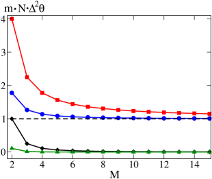
Figure 1: Ultimate scaling of the sensitivity for various non-linear potentials given by Eq. (20). Red squares, blue circles, black diamonds and green triangles correspond to $j=-2,-1,1,2$, respectively. The black dashed line denotes the sensitivity of a standard $j=1,M=2$ two-mode interferometer.

The behavior with $M$ of the r.h.s. of the above equation for various $j$ is show in Fig. 1. When $j>0$, $\Delta^{2}\theta$ continuously improves with increasing $M$, and the larger $j$ is, the quicker is the improvement. This would be the case – for instance – for the quadratic potential, i.e. $j=2$. On the other hand, when the potential decays with distance $j<0$, as is the case of the Casimir-Polder-type interactions which can exhibit the $j=-3$ or $j=-4$ scaling antezza ; chwed2 , there is no substantial gain from the multi-mode structure of the interferometer. This happens because already the phase imprinted on the second well, which is equal to $2^{-|j|}\theta$, is negligible when compared to $\theta$. In this case $\Delta^{2}\theta\geq\frac{1}{m}\frac{1}{N^{2}}$ and by increasing $M$ the sensitivity saturates to the value corresponding to a linear potential and two wells, since effectively only the first well experiences the action of the perturbing potential.

Apart from the ultimate scaling, it is interesting to derive an expression for the sensitivity for symmetric states, as was done in Section III.2 for linear potentials. The derivation does not change substantially with respect to the line of reasoning presented in Appendix A, with the only difference that the summations over the sites involve $k^{j}$ instead of $k$. The resulting sensitivity bound for symmetric states reads

$$\Delta^{2}\theta\geq\frac{1}{m}\frac{1}{f(N)}\frac{M^{2}}{4\left(M\rm{H}_{M}^{(-2j)}-(\rm{H}_{M}^{(-j)})^{2}\right)},$$ (21)

where $\rm{H}_{n}^{(r)}=\sum_{k=1}^{n}k^{-r}$ is known as the Harmonic number. For $j>0$ and a large number of lattice sites, the sensitivity bound can be approximated by

$$\Delta^{2}\theta\geq\frac{1}{m}\frac{1}{f(N)}\frac{1}{M^{2j}}\frac{(1+j)^{2}(1+2j)}{(2j)^{2}},$$ (22)

which shows that the $1/M^{j}$ improvement on $\Delta\theta$ is preserved for symmetric states.

We underline that – via Eq. (20) – the multi-mode interferometer could serve as a sensitive tool to determine the spatial dependence of the perturbing potential, which is a relevant task for instance in the determination of the Casimir-Polder force or deviations from the Newton law of gravity at the micrometer scale.

IV Sensitivity for the fit to the interference pattern

The QFI was used above to set the lower limit for the sensitivity by optimizing of $\Delta^{2}\theta$ with respect to the output measurement and estimator. Below we demonstrate that the scaling of the sensitivity with $M$, which is present in Eq. (17), is preserved even for a particularly simple phase estimation protocol, although the sensitivity does not saturate the QFI. Also the scaling with $N$ is preserved for the superfluid and phase-squeezed states.

We assume that after the system acquires the phase as in Eq. (5), the optical lattice is switched off and the wave-packets $\psi_{k}(x)$ – which were initially localized at each site – expand and in the far field form an interference pattern. Positions of atoms are recorded and the phase is estimated by fitting the density $\rho(x|\theta)=\langle\hat{\Psi}^{\dagger}(x|\theta)\hat{\Psi}(x|\theta)\rangle$ to the acquired data. In our past work chwed_njp we have shown that when this estimation protocol is employed, the sensitivity is given by

$$\Delta^{2}\theta=\frac{1}{m}\frac{F_{1}+C}{F_{1}^{2}},$$ (23)

where $F_{1}$ is the one-body Fisher information which reads

$$F_{1}=\int dx\frac{1}{\rho(x|\theta)}\left(\frac{\partial\rho(x|\theta)}{\partial\theta}\right)^{2}.$$ (24)

The coefficient $C$ depends both on the one- and two-body correlations,

$$C=\!\int\!\!dx\!\int\!\!dy\,G^{(2)}(x,y|\theta)\,\partial_{\theta}\log\left[\rho(x|\theta)\right]\,\partial_{\theta}\log\left[\rho(y|\theta)\right],$$ (25)

where $G^{(2)}(x,y|\theta)=\langle\Psi^{\dagger}(x|\theta)\hat{\Psi}^{\dagger}(y|\theta)\Psi(y|\theta)\hat{\Psi}(x|\theta)\rangle$. Our goal is to analyze how the sensitivity (23) depends on both the number of sites $M$ and the non-classical correlations present in the state (2).

In section III.2 we have seen that the usefully entangled states for the present interferometer have enhanced number fluctuations. In particular, the NOON state provides the best scaling with the number of particles $N$. This statement, however, assumes that we are always able to perform the optimal measurement, which in general depends itself on the input state. In this section instead we fix the measurement (as described above), and study the behavior of the sensitivity for different states characterized by enhanced number fluctuations (we will see that such states are still the useful ones also for the particular measurement considered). For two lattice sites ($M=2$), one can easily generate a family of such usefully entangled states by numerically finding the ground state of the two-well Bose-Hubbard Hamiltonian

$$\hat{H}_{\rm BH}=-E_{J}\hat{J}_{x}+U\hat{J}_{z}^{2}$$ (26)

with $U<0$. Here, $E_{J}$ is the Josephson energy, related to the frequency of the inter-well tunneling, and $U$ is the amplitude of the on-site two-body interactions. This procedure for generating the input states is also relevant for the setup we consider, since it will correspond to adiabatical preparation in the lattice. To perform an analogous calculation for higher $M$ is very demanding, since the dimensionality of the Hilbert space grows rapidly, as indicated by multiple sums present in Eq. (1). This difficulty can be overcome by replacing the true state (1) with

$$|\psi\rangle=\bigotimes_{k=1}^{M}\sum_{n_{k}=0}^{\infty}C_{n_{k}}|n_{k}\rangle.$$ (27)

This is the Gutzwiller approximation of the quantum state of the bosons (see rmp_zw and references therein). The number of atoms is not fixed anymore, and thus each site is independent from the others. Although such state does not recover correlations among the wells, it can be used to mimic non-classical correlations by increasing the on-site atom number variance $\Delta^{2}\hat{n}$. In analogy to the fixed-$N$ case (2) we assume that the average number of atoms per site is $\langle\hat{n}_{k}\rangle=\frac{N}{M}$, so that the average number of atoms in the whole system is $N$.

We express the field operator $\hat{\Psi}(x|\theta)$ in the far field,

$$\hat{\Psi}(x|\theta)=\tilde{\psi}\left(\frac{x}{\tilde{\sigma}^{2}}\right)\sum_{k=1}^{M}e^{-i\phi(x)\cdot k}\hat{a}_{k}.$$ (28)

We assumed that initially all the wave-packets $\psi_{k}(x)$ had identical shape but were localized around separated sites of the optical lattice. The function $\tilde{\psi}$ is the Fourier transform of $\psi_{k}(x)$, which is common for each well, and $\tilde{\sigma}=\sqrt{\frac{\hbar t}{\mu}}$ ($\mu$ is the atomic mass and $t$ is the expansion time). The phase factor is defined as

$$\phi(x)=2\frac{x_{0}}{\tilde{\sigma}^{2}}x+\theta$$ (29)

where $x_{0}$ is the lattice spacing first introduced below Eq. (4).

The density $\rho(x|\theta)$ obtained using Equations (27) and (28) is

$$\rho(x|\theta)=\langle\psi|\hat{\Psi}^{\dagger}(x|\theta)\hat{\Psi}(x|\theta)|\psi\rangle=N\Big{|}\tilde{\psi}\left(\frac{x}{\tilde{\sigma}^{2}}\right)\Big{|}^{2}\cdot f(x|\theta),$$ (30)

where $|\tilde{\psi}|^{2}$ is the envelope of the interference pattern, while the fringes are contained in

$$f(x|\theta)=1+\frac{\langle\hat{a}\rangle^{2}}{N}\left(\frac{\sin^{2}\left(\frac{M\phi(x)}{2}\right)}{\sin^{2}\left(\frac{\phi(x)}{2}\right)}-M\right).$$ (31)

The density is put into Eq. (24), giving

$$F_{1}=N\int dx\Big{|}\tilde{\psi}\left(\frac{x}{\tilde{\sigma}^{2}}\right)\Big{|}^{2}\frac{1}{f(x|\theta)}\left(\frac{\partial f(x|\theta)}{\partial\theta}\right)^{2}.$$ (32)

When the density of the interference pattern consists of many fringes, the envelope $|\tilde{\psi}|^{2}$ varies much slower in $x$ then the function $f(x|\theta)$. An integral of a slowly varying envelope with a quickly oscillating periodic function can be split into a product of an integral of the envelope alone times the average value of the quickly changing $f(x|\theta)$. Since the envelope is normalized, we immediately get

$$F_{1}=N\int_{0}^{2\pi}\frac{d\phi}{2\pi}\frac{1}{f(\phi)}\left(\frac{\partial f(\phi)}{\partial\phi}\right)^{2},$$ (33)

where $\phi$ was defined in Eq. (29). This integral depends on the quantum state through the average value $\langle\hat{a}\rangle$, as can be seen from Eq. (30). Apart from the analytical case $M=2$, its value has to be calculated numerically.

Now we have to calculate the coefficient $C$, which in turn requires to compute the second-order correlation function. After a lengthy calculation we obtain (see Appendix B for details)

$$\!\!\!\!\!\!\!\!\!C = \left[\langle\hat{a}^{2}\rangle^{2}\!-\!\left(\frac{N}{M}\right)^{2}\!+\!2\frac{N}{M}\langle\hat{a}\rangle^{2}\!-\!2\langle\hat{a}^{2}\rangle\langle\hat{a}\rangle^{2}\right]I_{1}$$ (34a)

$$+ \left[2\langle\hat{a}^{2}\rangle\langle\hat{a}\rangle^{2}-2\frac{N}{M}\langle\hat{a}\rangle^{2}\right]I_{2}.$$ (34b)

where the two integrals are given by

$$I_{1} = \int_{-\pi}^{\pi}\frac{d\phi}{2\pi}\int_{-\pi}^{\pi}\frac{d\phi^{\prime}}{2\pi}\ \partial_{\theta}\log\left[f(\phi)\right]\partial_{\theta}\left[f(\phi^{\prime})\right]$$ (35a)

$$\times \frac{\cos[M(\phi+\phi^{\prime})]-1}{\cos[\phi+\phi^{\prime}]-1}$$ (35b)

and

$$I_{2} = \int_{-\pi}^{\pi}\frac{d\phi}{2\pi}\int_{-\pi}^{\pi}\frac{d\phi^{\prime}}{2\pi}\ \partial_{\theta}\log\left[f(\phi)\right]\partial_{\theta}\left[f(\phi^{\prime})\right]$$ (36a)

$$\times \frac{\sin\left[\frac{M}{2}\phi\right]\sin\left[\frac{M}{2}\phi^{\prime}\right]\sin\left[\frac{M}{2}(\phi+\phi^{\prime})\right]}{\sin\left[\frac{\phi}{2}\right]\sin\left[\frac{\phi^{\prime}}{2}\right]\sin\left[\frac{\phi+\phi^{\prime}}{2}\right]}.$$ (36b)

As a first test of Equations (33) and (34), in the next section we show that for $M=2$ we recover a known analytical expression for the sensitivity obtained using a two-mode state with fixed $N$ chwed_njp .

IV.1 Fit sensitivity with two lattice sites

To make a direct comparison, we start by recalling the main result of our previous work chwed_njp , where we focused on phase estimation with a fixed-$N$ two-mode state $|\psi\rangle=\sum_{n=0}^{N}C_{n}|n,N-n\rangle$. In the resulting $N$ qbits space, every possible interferometric operation can be mapped into a rotation, with the angular momentum operators $\hat{J}_{x}=\frac{1}{2}(\hat{a}^{\dagger}\hat{b}+\hat{a}\hat{b}^{\dagger})$, $\hat{J}_{y}=\frac{1}{2i}(\hat{a}^{\dagger}\hat{b}-\hat{a}\hat{b}^{\dagger})$ and $\hat{J}_{z}=\frac{1}{2}(\hat{a}^{\dagger}\hat{a}-\hat{b}^{\dagger}\hat{b})$. We have shown that when the phase is deduced from the fit of the one-body density to the interference pattern formed by two expanding wave-packets, the sensitivity (23) can be expressed in terms of two quantities. One is the spin-squeezing parameter grond , which is a measure of entanglement related to the phase-squeezing of $|\psi\rangle$ and reads $\xi_{\phi}=\sqrt{N\frac{\Delta^{2}\hat{J}_{y}}{\langle\hat{J}_{x}\rangle^{2}}}$. The other is the visibility of the interference fringes, $\nu=\frac{2}{N}\langle\hat{J}_{x}\rangle$. The sensitivity

$$\Delta^{2}\theta=\frac{1}{mN}\left[\xi_{\phi}^{2}+\frac{\sqrt{1-\nu^{2}}}{\nu^{2}}\right]$$ (37)

results from the interplay between the growing entanglement ($\xi^{2}_{\phi}\rightarrow 0$) and the loss of the visibility ($\nu\rightarrow 0$). Naturally, there is some optimally squeezed state, which gives the minimal value of $\Delta^{2}\theta$, as discussed in detail in chwed_njp .

We now calculate the sensitivity (23) using the Gutzwiller approximation (27) for two wells, and check how it compares with the exact result (37). As shown in the Appendix C, in this case, both the one body Fisher information (33) and the coefficient $C$ (34) can be evaluated analytically and the outcome is

$$\Delta^{2}\theta=\frac{1}{mN}\left[\tilde{\xi}_{\phi}^{2}+\frac{\sqrt{1-\tilde{\nu}^{2}}}{\tilde{\nu}^{2}}\right],$$ (38)

where the tilde sign denotes the phase-squeezing parameter and the visibility calculated with a product state. Although Equations (37) and (38) have identical form, we still have to verify whether the two-well entanglement of the fixed-$N$ state can be reproduced with a product state by increasing the on-site fluctuations. We model the coefficients of Eq. (27) with a Gaussian

$$C_{n_{k}}\propto e^{-\frac{\left(n_{k}-\langle n\rangle\right)^{2}}{2\sigma^{2}}},$$ (39)

where $\langle n\rangle=\frac{N}{2}$ for a two-mode state. The on-site atom number variance is simply $\Delta^{2}\hat{n}=\sigma^{2}$, thus a coherent superfluid state can be modeled by setting the fluctuations at the Poissonian level, i.e. $\sigma=\sqrt{N}$. To check if Eq. (38) will drop below the SNL when the fluctuations are super-Poissonian, we proceed as follows. For various values of $\sigma>\sqrt{N}$ we calculate the phase-squeezing parameter $\tilde{\xi}_{\phi}^{2}$ and the visibility $\tilde{\nu}$ and plot the sensitivity (38) as a function of $\tilde{\xi}_{\phi}^{2}$. To compare with the fixed-$N$ case, we find the ground state of the Hamiltonian (26) for various values of the ratio $\frac{E_{J}}{U}<0$. For every state found in this way, we calculate the phase-squeezing parameter $\xi_{\phi}^{2}$ and the visibility $\nu$ and on the same plot draw the sensitivity (37) as a function of $\xi_{\phi}^{2}$. Figure 2 shows that not only Equations (38) and (37) have identical form but also the quantum correlations giving sub shot-noise sensitivity can be perfectly mimicked using a product state (27) with large on-site atom number fluctuations. In both cases, the sensitivity has an optimal point, where the entanglement is balanced by the fringe visibility. Clearly, the Gutzwiller approximation gets worse when the correlations between different wells increase (that is, going further to the left in Fig. 2), but for the usefully states we consider and for this particular choice of the measurement, it is exact for all practical purposes.

Having proven its usefulness, in the following section we employ the Gutzwiller ansatz (27) plus the Gaussian approximation on the coefficient of the product state (39) in order to analyze how the sensitivity (23) behaves for higher $M$, where results from a fixed-$N$ model are unavailable.

Figure 2: The sensitivity $m\cdot N\cdot\Delta^{2}\theta$ of the parameter estimation from the fit to the density of the interference pattern with $M=2$ and $N=200$ calculated using the state with fixed- (open blue circles) and non-fixed number of atoms (solid black line) as a function of the phase-squeezing parameter. The sensitivities shown are normalized to the SNL. The dashed red line shows the ultimate precision of the phase estimation given by the QFI from Eq. (15). The horizontal black dotted line shows the shot noise limit.

IV.2 Fit sensitivity with $M$ lattice sites

For $M>2$, when the integrals (33), (35) and (36) cannot be evaluated analytically, we calculate the sensitivity (23) numerically. We fix the average total number of atoms to be $\langle\hat{N}\rangle=5\times 10^{4}$ and for a given $M$ we calculate the sensitivity (23) for different values of the on-site atom-number fluctuations using the Gaussian model (39) with $\langle n\rangle=\frac{\langle\hat{N}\rangle}{M}$. In order to compare the results for different $M$, we normalize the sensitivity by the factor $\frac{1}{3}(M^{2}-1)$, that is, by the sensitivity achieved with the best possible measurement (17) at the shot-noise level. In Fig. 3 we plot $m\langle\hat{N}\rangle\times\frac{1}{3}(M^{2}-1)\Delta^{2}\theta$ for $M=2,4,6,8,10$ and 12. The outcome is – with a high level of accuracy – independent of $M$. We thus conclude that the sensitivity of the fit has a form similar to (17), i.e.

$$\Delta^{2}\theta=\frac{1}{m}\frac{1}{\zeta(\langle\hat{N}\rangle)}\frac{3}{(M^{2}-1)},$$ (40)

where $\zeta(\langle\hat{N}\rangle)$ is some function of the average total number of atoms, which becomes larger for states with increased on-site atom number fluctuations, $\zeta>\langle\hat{N}\rangle$.

Figure 3: (color online) The sensitivity $m\cdot N\cdot\Delta^{2}\theta$ of the parameter estimation from the fit to the density of the interference pattern for $M=2,4,6,8,10$ and 12 (different color solid lines) with a fixed average number of atoms equal to $\langle N\rangle=5\times 10^{4}$. The sensitivities shown are normalized to the SNL and multiplied by the factor $\frac{1}{3}(M^{2}-1)$. The dashed red line shows the ultimate precision of the phase estimation given by the QFI from Eq. (15). The horizontal black dotted line shows the shot noise limit.

In Fig. 3, as the phase-squeezing parameter drops, the discrepancy between the curves calculated for different $M$ grows. This is a spurious result due to the Gutzwiller approximation (27) for the state $|\psi\rangle$. When the average number of atoms in the system is fixed and $M$ is changed, the average on-site occupation varies. This is not a problem for as long as the width $\sigma$ of the Gaussian (39) is small as compared to $\langle\hat{n}\rangle$. However, we increase $\sigma$ to mimic the growing entanglement in the system. Once $\sigma$ is comparable to $\langle\hat{n}\rangle$, the change in the on-site population for different $M$ becomes relevant. Therefore, by changing $M$ we are actually changing the nature of the quantum state and, in particular, we cannot assume that the squeezing parameter remains fixed. One could avoid this problem by – rather than fixing $\langle N\rangle$ – fixing the on-site population $\langle n\rangle$ and increase the number of wells so that $\langle N\rangle=M\langle n\rangle$.

V Conclusions

We have analyzed the performance of ultracold bosons trapped inside an optical lattice as an interferometric device for the measurement of spatially dependent forces. For a potential $g\,x^{j}$ with $j>0$, we showed that, optimizing over all possible output measurements, the coupling constant $g$ can be measured with an uncertainty $\Delta g$ scaling like $M^{-j}$, for a large number of lattice sites $M$, and independent of the quantum state employed. We then showed that this scaling with the number of lattice sites can still be reached with a particular output measurement which is commonly employed with ultracold atoms: a least square fit to the interference pattern resulting from the overlap o the freely expanding atoms released from the confining potential. We also derived the improvements coming from entangling the quantum state.

The device here studied is an example of a matter-wave multi-path interferometer. While the sensitivity bounds for a general two-path interferometer are already largely studied, the same analysis based on rigorous estimation theory results has not yet been performed for multi-path devices. Moreover, the potential of the implementation of these devices with atoms seems very promising, due to the growing control and tunability of the available trapping and probing tools, especially for ultracold atoms.

Finally, we underline that the precision of the time-of-flight interferometer, where the phase is estimated from the fit of the averaged density to the measured interference pattern cannot be surpassed by adding a hopping term to the generating Hamiltonian (4). The presence of the hopping – which induces the Bloch oscillations – is an extra complication, which changes the optimal states depending on the ratio between the tunneling energy to the phase related energy $\epsilon$, but does not introduce any further benefit. Some of these conclusions can be found in chwed2 and will be discussed in detail elsewhere.

VI Acknowledgments

We thank A. Recati for some very useful remarks. J. Ch. acknowledges Foundation for Polish Science International TEAM Program co-financed by the EU European Regional Development Fund and the support of the National Science Centre. F.P. acknowledges support by the Alexander Von Humboldt foundation. A.S. acknowledges support of the EU-STREP Project QIBEC. QSTAR is the MPQ, IIT, LENS, UniFi joint center for Quantum Science and Technology in Arcetri.

Appendix A Calculation of the QFI

In order to calculate the $F_{Q}$, we need to derive an expression for the variance of the operator $\hat{h}$. Using the definition (6), we get

$$\langle\hat{h}^{2}\rangle=\sum_{k_{1},k_{2}}k_{1}k_{2}\langle\hat{n}_{k_{1}}\hat{n}_{k_{2}}\rangle=\sum_{k}k^{2}\langle\hat{n}_{k}^{2}\rangle+\sum_{k_{1}\neq k_{2}}k_{1}k_{2}\langle\hat{n}_{k_{1}}\hat{n}_{k_{2}}\rangle.$$ (41)

We now make of the symmetry between the wells. The average value $\langle\hat{n}_{k}^{2}\rangle$ does not depend on index $k$ and thus can be denoted as $\langle\hat{n}^{2}\rangle$. The same argument concerns the inter-well correlation $\langle\hat{n}_{k_{1}}\hat{n}_{k_{2}}\rangle$, which will be denoted as $\langle\hat{n}_{i}\hat{n}_{j}\rangle$, where $i,j$ are indeces of any two sites. The above expression thus boils down to

$$\langle\hat{h}^{2}\rangle=\langle n^{2}\rangle\sum_{k}k^{2}+\langle\hat{n}_{i}\hat{n}_{j}\rangle\sum_{k_{1}\neq k_{2}}k_{1}k_{2}=$$ (42)

$$\frac{M}{6}(M+1)(2M+1)\langle\hat{n}^{2}\rangle+\langle\hat{n}_{i}\hat{n}_{j}\rangle\frac{M}{12}(M^{2}-1)(3M+2).$$

Our next step is to show that $\langle\hat{n}_{i}\hat{n}_{j}\rangle$ can be written as a function of $\langle\hat{n}^{2}\rangle$ only. To this end, since the state is symmetric, we can take $i=1$ and $j=M$ and obtain

$$\langle\hat{n}_{1}\hat{n}_{M}\rangle = \sum_{\vec{n}}C_{\vec{n}}^{2}\,n_{1}\cdot(N-n_{1}-\ldots-n_{M-1})$$ (43)

$$= \frac{N^{2}}{M}-\sum_{\vec{n}}C_{\vec{n}}^{2}\,n_{1}\cdot(n_{1}+\ldots+n_{M-1}).$$ (44)

Now, since it doesn’t matter which two wells we correlate, in the sum instead of $n_{1}$ we can use an average over $M-1$ wells as follows

$$\langle\hat{n}_{1}\hat{n}_{2}\rangle=\frac{N^{2}}{M}-\sum_{\vec{n}}C_{\vec{n}}^{2}\,\frac{n_{1}+\ldots+n_{M-1}}{M-1}\cdot(n_{1}+\ldots+n_{M-1}).$$ (45)

Finally, we exploit the fact that the total number of atoms is fixed and thus $n_{1}+\ldots+n_{M-1}=N-n_{M}$ and obtain

$$\langle\hat{n}_{1}\hat{n}_{M}\rangle = \frac{N^{2}}{M}-\sum_{\vec{n}}C_{\vec{n}}^{2}\,\frac{(N-n_{M})^{2}}{M-1}$$ (46)

$$= \frac{N^{2}}{M}-\frac{\langle n^{2}\rangle-2N^{2}/M+N^{2}}{M-1}.$$ (47)

Using the result for the average value of $\hat{h}$, we finally obtain

$$F_{Q}=4\Delta^{2}\hat{h}=\frac{1}{3}(M+1)M^{2}\Delta^{2}\hat{n},$$ (48)

where $\Delta^{2}\hat{n}=\langle\hat{n}^{2}\rangle-\langle\hat{n}\rangle^{2}$ is the on-site variance.

Appendix B Calculation of the sensitivity

In this Appendix we give details of derivation of coefficient $C$ from Eq. (34) which is used to evaluate the sensitivity (23) using the product state (27). In order to calculate $C$, one first has to find the second order correlation function,

$$G^{(2)}(x,y|\theta)=\langle\hat{\Psi}^{\dagger}(x|\theta)\hat{\Psi}^{\dagger}(y|\theta)\hat{\Psi}(y|\theta)\hat{\Psi}(x|\theta)\rangle.$$ (49)

When the field operator, which is introduced in Eq. (28), is put into this definition, we obtain

$$G^{(2)}(x,y|\theta)=\Big{|}\tilde{\psi}\left(\frac{x}{\tilde{\sigma}^{2}}\right)\Big{|}^{2}\Big{|}\tilde{\psi}\left(\frac{y}{\tilde{\sigma}^{2}}\right)\Big{|}^{2}\times$$ (50)

$$\!\!\!\sum_{k_{1},k_{2},k_{3},k_{4}=1}^{M}\!\!\!\!\!\!e^{i\phi(x)(k_{1}-k_{4})}e^{i\phi(y)(k_{2}-k_{3})}\langle\hat{a}^{\dagger}_{k_{1}}\hat{a}^{\dagger}_{k_{2}}\hat{a}_{k_{3}}\hat{a}_{k_{4}}\rangle,$$ (51)

where $\phi(x)=2\frac{x_{0}}{\tilde{\sigma}^{2}}x+\theta$. The above sum cannot be performed in a straightforward manner, since special care has to be taken to distinguish cases when the indices $k_{1}\ldots k_{4}$ in the average value $\langle\hat{a}^{\dagger}_{k_{1}}\hat{a}^{\dagger}_{k_{2}}\hat{a}_{k_{3}}\hat{a}_{k_{4}}\rangle$ are equal or different from each other. A careful classification of all the possible terms gives

$$G^{(2)}(x,y|\theta)=\Big{|}\tilde{\psi}\left(\frac{x}{\tilde{\sigma}^{2}}\right)\Big{|}^{2}\Big{|}\tilde{\psi}\left(\frac{y}{\tilde{\sigma}^{2}}\right)\Big{|}^{2}\times\left\{M\langle\hat{a}^{\dagger}\hat{a}^{\dagger}\hat{a}\hat{a}\rangle+(f(x+y)-M)\langle\hat{a}^{\dagger}\hat{a}^{\dagger}\rangle^{2}+\langle\hat{n}\rangle^{2}(f(x-y)+M^{2})\right.$$ (52a)

$$+2\left[f(x)+f(y)-2M\right]\langle\hat{a}^{\dagger}\hat{a}^{\dagger}\hat{a}\rangle\langle\hat{a}\rangle+\langle\hat{n}\rangle\langle\hat{a}\rangle^{2}\left[8M-2M^{2}+(M-4)\left(f(x)+f(y)\right)-2f(x-y)+2g(x,-y)\right]$$ (52b)

$$+\langle\hat{a}\rangle^{2}\langle\hat{a}^{2}\rangle\left[4M-2f(x)-2f(y)-2f(x+y)+2g(x,y)\right]$$ (52c)

$$\left.+\langle\hat{a}\rangle^{4}\left[f(x)f(y)-(M-4)(f(x)+f(y))+f(x+y)+f(x-y)-2g(x,y)-2g(x,-y)+M^{2}-6M\right]\right\}.$$ (52d)

The function $f(x)$ is defined as

$$f(x)=\frac{\cos\left[M\phi(x)\right]-1}{\cos\left[\phi(x)\right]-1},$$ (53)

while the $g(x,y)$ function is

$$g(x,y)=\frac{\sin\left[\frac{M\phi(x)}{2}\right]\sin\left[\frac{M\phi(y)}{2}\right]\sin\left[\frac{M(\phi(x)+\phi(y))}{2}\right]}{\sin\left[\frac{\phi(x)}{2}\right]\sin\left[\frac{\phi(y)}{2}\right]\sin\left[\frac{\phi(x)+\phi(y)}{2}\right]}.$$ (54)

The coefficient $C$ is defined as a double integral of the above second order correlation function with the one-body probabilities calculated at positions $x$ and $y$, namely

$$C=\!\int\!\!dx\!\int\!\!dy\,G^{(2)}(x,y|\theta)\,\partial_{\theta}\log\left[\rho(x|\theta)\right]\,\partial_{\theta}\log\left[\rho(y|\theta)\right].$$ (55)

The one-body density is defined in Eq. (30). We use the fact that the interference pattern consists of many fringes, so that the envelope $|\tilde{\psi}|^{2}$ varies slowly as compared to the oscillatory functions present in $f$, $g$ and the density $\rho$. Therefore, the integral (55) can be rewritten as

$$C = \!\int_{-\pi}^{\pi}\frac{d\phi}{2\pi}\int_{-\pi}^{\pi}\frac{d\phi^{\prime}}{2\pi}\,G^{(2)}(\phi,\phi^{\prime}|\theta)$$ (56a)

$$\times \partial_{\theta}\log\left[\rho(\phi|\theta)\right]\,\partial_{\theta}\log\left[\rho(\phi^{\prime}|\theta)\right],$$ (56b)

where we changed the variables $x\rightarrow\phi$ and $y\rightarrow\phi^{\prime}$. It can be demonstrated that

$$\int_{-\pi}^{\pi}\frac{d\phi}{2\pi}\partial_{\theta}\log\left[\rho(\phi|\theta)\right]=0,$$ (57a)

therefore all the terms from Equations (52) which do not depend on both $\phi$ and $\phi^{\prime}$ are zero. Using a property of the functions $f$ and $g$

$$\int_{-\pi}^{\pi}\frac{d\phi}{2\pi}\int_{-\pi}^{\pi}\frac{d\phi^{\prime}}{2\pi}f(\phi+\phi^{\prime})\partial_{\theta}\log\left[\rho(\phi|\theta)\right]\,\partial_{\theta}\log\left[\rho(\phi^{\prime}|\theta)\right]=$$

$$-\int_{-\pi}^{\pi}\frac{d\phi}{2\pi}\int_{-\pi}^{\pi}\frac{d\phi^{\prime}}{2\pi}f(\phi-\phi^{\prime})\partial_{\theta}\log\left[\rho(\phi|\theta)\right]\,\partial_{\theta}\log\left[\rho(\phi^{\prime}|\theta)\right]$$

and the same with $g(\phi,\phi^{\prime})$ and $g(\phi,-\phi^{\prime})$ we finally get

$$\!\!\!\!\!C = \left[\langle\hat{a}^{2}\rangle^{2}-\langle\hat{n}\rangle^{2}+2\langle\hat{n}\rangle\langle\hat{a}\rangle^{2}-2\langle\hat{a}^{2}\rangle\langle\hat{a}\rangle^{2}\right]\times$$ (58a)

$$\times \int_{-\pi}^{\pi}\frac{d\phi}{2\pi}\int_{-\pi}^{\pi}\frac{d\phi^{\prime}}{2\pi}\frac{p^{\prime}(\phi)}{p(\phi)}\frac{p^{\prime}(\phi^{\prime})}{p(\phi^{\prime})}f(\phi+\phi^{\prime})$$ (58b)

$$+ \left[2\langle\hat{a}^{2}\rangle\langle\hat{a}\rangle^{2}-N\langle\hat{a}\rangle^{2}\right]\times$$ (58c)

$$\times \int_{-\pi}^{\pi}\frac{d\phi}{2\pi}\int_{-\pi}^{\pi}\frac{d\phi^{\prime}}{2\pi}\frac{p^{\prime}(\phi)}{p(\phi)}\frac{p^{\prime}(\phi^{\prime})}{p(\phi^{\prime})}g(\phi,\phi^{\prime}),$$ (58d)

which coincides with Eq. (34).

Appendix C Sensitivity for two wells

First, we calculate the one-body Fisher information defined in Eq. (33). For $M=2$ the $f$ function from Eq. (31) reads

$$f(\phi)=1+\tilde{\nu}\cos\phi,$$ (59)

where $\tilde{\nu}$ is the fringe visibility calculated with a product state,

$$\tilde{\nu}=\frac{2}{N}\langle\hat{J}_{x}\rangle=\frac{2}{N}\frac{\langle\hat{a}^{\dagger}\rangle\langle\hat{b}\rangle+\langle\hat{a}\rangle\langle\hat{b}^{\dagger}\rangle}{2}=\frac{2}{N}\langle\hat{a}\rangle^{2},$$ (60)

where we used the symmetry between the two wells, and the last step was possible because the coefficients $C_{n}$ are taken to be real. We insert (59) into (33) and obtain an analytical outcome

$$F_{1}=1-\sqrt{1-\tilde{\nu}^{2}}.$$ (61)

The integrals $I_{1}$ from Eq. (35) and $I_{2}$ from Eq. (36) can be calculated in a similar way, giving

$$I_{1}=I_{2}=\frac{2}{\tilde{\nu}^{2}}(-2+\tilde{\nu}^{2}+2\sqrt{1-\tilde{\nu}^{2}}).$$ (62)

As a result the coefficient $C$ from Eq. (34) for $M=2$ reads

$$C=\frac{2}{\tilde{\nu}^{2}}(-2+\tilde{\nu}^{2}+2\sqrt{1-\tilde{\nu}^{2}})\left[\langle\hat{a}^{2}\rangle^{2}-\frac{N^{2}}{4}\right].$$ (63)

Finally, we note that for a symmetric state $\langle\hat{J}_{y}\rangle=0$, thus the variance of the $\hat{J}_{y}$ operator calculated using a product state reads

$$\Delta^{2}\hat{J}_{y}=\frac{1}{2}\left[\frac{N^{2}}{4}+\frac{N}{2}-\langle\hat{a}^{2}\rangle^{2}\right],$$ (64)

which allows to rewrite Eq. (63) in a following way

$$C=\frac{4}{\tilde{\nu}^{2}}(-2+\tilde{\nu}^{2}+2\sqrt{1-\tilde{\nu}^{2}})\left[\frac{N}{4}-\tilde{\Delta}^{2}\hat{J}_{y}\right].$$ (65)

Combining (61) and (65) as in Eq. (23) we obtain

$$\Delta^{2}\theta=\frac{1}{mN}\left[\tilde{\xi}_{\phi}^{2}+\frac{\sqrt{1-\tilde{\nu}^{2}}}{\tilde{\nu}^{2}}\right],$$ (66)

where $\tilde{\xi}_{\phi}^{2}$ is the phase-squeezing parameter calculated with a product state.

References

- (1) V. Giovanetti, S. Lloyd and L. Maccone, Science 306, 1330 (2004)
- (2) A. D. Cronin, J. Schmiedmayer and D. E. Pritchard, Rev. Mod. Phys. 81, 1051 (2009)
- (3) T. A. Pasquini, et al., Phys. Rev. Lett. 93, 223201 (2004)
- (4) Y. J. Lin, et al., Phys. Rev. Lett. 92, 050404 (2004)
- (5) J. M. Obrecht, et al., Phys. Rev. Lett. 98, 063201 (2007)
- (6) B. P. Anderson, and M. A. Kasevich, Science 282, 1686 (1998)
- (7) M. Fattori, et al., Phys. Rev. Lett. 100, 080405 (2008)
- (8) F. Baumgärtner, et al., Phys. Rev. Lett. 105, 243003 (2010)
- (9) D. Leibfried et al, Science 304, 1476 (2004)
- (10) J. Appel et al, PNAS 106, 10960 (2009)
- (11) M. H. Schleier-Shmith et al, Phys. Rev. Lett. 104, 073604 (2010)
- (12) C. Gross, et al., Nature 464, 1165 (2010)
- (13) J. Estève, et al., Nature 455, 1216 (2008)
- (14) M. F. Riedel, et al., Nature 464, 1170 (2010)
- (15) K. Maussang, et al., Phys. Rev. Lett. 105, 080403 (2010)
- (16) B. Lücke, et al., Science 11, 773 (2011)
- (17) J. Appel, et al. , PNAS 106, 10960 (2009)
- (18) Zilong Chen, et al. , Phys. Rev. Lett. 106, 133601 (2011)
- (19) F. Zernike, J. Opt. Soc. Am. 40, 326 (1950)
- (20) G. M. D’Ariano and M. G. A. Paris, Phys. Rev. A 55, 2267 (1997)
- (21) B. C. Sanders, et al., J. Phys. A 32, 7791 (1999)
- (22) J. Söderholm, et al., Phys. Rev. A 67, 053803 (2003)
- (23) A. Vourdas, and J. A. Dunningham, Phys. Rev. A 71, 013809 (2005)
- (24) J. J. Cooper, et al., Phys. Rev. Lett. 108, 030402 (2012)
- (25) J. Petrovic, I. Herrera, P. Lombardi and F. S. Cataliotti, arxiv:1111.4321v1
- (26) C. Gross, et al., Phys. Rev. A 84, 011609(R) (2011)
- (27) I. Bloch, J. Dalibard and W. Zwerger, Rev. Mod. Phys. 80, 885 (2008)
- (28) M. Greiner, O. Mandel, T. Esslinger, T. W. Hänsch and I. Bloch, Nature 415, 39 (2002)
- (29) S. Fölling, F. Gerbier, A. Widera, O. Mandel, T. Gericke and I. Bloch, Nature 434, 481 (2005)
- (30) J. Chwedeńczuk, P. Hyllus, F. Piazza and A. Smerzi, New J. Phys. 14 093001 (2012)
- (31) S. L. Braunstein and C. M. Caves, Phys. Rev. Lett. 72, 3439 (1994).
- (32) J. Grond , U. Hohenester , I. Mazets and J. Schmiedmayer, New J. Phys. 12, 065036 (2010)
- (33) M. Antezza, L. P. Pitaevskii, and S. Stringari, Phys. Rev. A 70, 053619 (2004)
- (34) J. Chwedeńczuk, L. Pezzé, F. Piazza, and A. Smerzi, Phys. Rev. A 82, 032104 (2010)