Full Rank Solutions for the MIMO Gaussian Wiretap Channel with an Average Power Constraint

Abstract

This paper considers a multiple-input multiple-output (MIMO) Gaussian wiretap channel model, where there exists a transmitter, a legitimate receiver and an eavesdropper, each equipped with multiple antennas. In this paper, we first revisit the rank property of the optimal input covariance matrix that achieves the secrecy capacity of the multiple antenna MIMO Gaussian wiretap channel under the average power constraint. Next, we obtain necessary and sufficient conditions on the MIMO wiretap channel parameters such that the optimal input covariance matrix is full-rank, and we fully characterize the resulting covariance matrix as well. Numerical results are presented to illustrate the proposed theoretical findings.

EDICS: WIN-PHYL, WIN-INFO, MSP-CAPC, WIN-CONT

I Introduction

The broadcast nature of a wireless medium makes it very susceptible to eavesdropping, where the transmitted message is decoded by unintended receiver(s). Recent information-theoretic research on secure communication has focused on enhancing security at the physical layer. The wiretap channel, first introduced and studied by Wyner [1], is the most basic physical layer model that captures the problem of communication security. Wyner showed that when an eavesdropper’s channel is a degraded version of the main channel, the source and destination can achieve a positive secrecy rate, while ensuring that the eavesdropper gets zero bits of information. The maximum secrecy rate from the source to the destination is defined as the secrecy capacity. The Gaussian wiretap channel, in which the outputs at the legitimate receiver and at the eavesdropper are corrupted by additive white Gaussian noise, was studied in [2].

Determining the secrecy capacity of a Gaussian wiretap channel is in general a difficult non-convex optimization problem, and has been addressed independently in [3]-[9]. Oggier and Hassibi [3] and Khisti and Wornell [4] followed an indirect approach using a Sato-like argument and matrix analysis tools. They considered the problem of finding the secrecy capacity of the Gaussian MIMO wiretap channel under the average total power constraint, and a closed-form expression for the secrecy capacity in the high signal-to-noise-ratio (SNR) regime was obtained in [4]. In [5], the rank property of the optimal input covariance matrix for the secrecy rate maximization problem is discussed but the authors were unable to characterize the solution for the general case. For some special cases of the MIMO wiretap channel, where the solution has rank one, the optimal input covariance matrix that achieves the secrecy capacity under the average total power constraint was obtained in [5]-[7].

In [8], Liu and Shamai propose a more information-theoretic approach using the enhancement concept, originally presented by Weingarten et al. [10], as a tool for the characterization of the MIMO Gaussian broadcast channel capacity. Liu and Shamai have shown that an enhanced degraded version of the channel attains the same secrecy capacity as does a Gaussian input distribution. From the mathematical solution in [8] it was evident that such an enhanced channel exists; however it was not clear how to construct such a channel until the work of [9], which provided a closed-form expression for the secrecy capacity under a covariance matrix power constraint. While this result is interesting since the expression for the secrecy capacity is valid for all SNR scenarios, there still exists no computable secrecy capacity expression for the MIMO Gaussian wiretap channel under an average total power constraint.

In this paper, we first investigate the rank property of the optimal input covariance matrix that achieves the secrecy capacity of the general Gaussian multiple-input multiple-output (MIMO) wiretap channel under the average total power constraint, where the number of antennas is arbitrary for both the transmitter and the two receivers. Next, we obtain the optimal input covariance matrix for the case that this optimal covariance matrix is full-rank. Necessary and sufficient conditions to have a full-rank optimal input covariance matrix are characterized as well.

The rest of this paper is organized as follows. In the next section, we describe the assumed mathematical model and revisit the current solution for the wiretap channel under the matrix power constraint. The rank property of the optimal input covariance matrix under the average power constraint is investigated in Section III, and in Section IV we characterize the conditions under which the input covariance matrix that achieves the secrecy capacity of a wiretap channel under the average power constraint is full-rank. In Section V, we discuss some interesting facts regarding the optimal solution, and in Section VI we present numerical results to illustrate the proposed solutions. Finally, Section VII concludes the paper.

Notation: Vector-valued random variables are written with non-boldface uppercase letters (e.g., $X$), while the corresponding non-boldface lowercase letter (${\mathbf{x}}$) denotes a specific realization of the random variable. Scalar variables are written with non-boldface (lowercase or uppercase) letters. The Hermtian (i.e., conjugate) transpose is denoted by $(.)^{H}$, the matrix trace by Tr(.), and I indicates an identity matrix. Inequality ${\mathbf{A}}\preceq{\mathbf{B}}$ means that ${\mathbf{A}}-{\mathbf{B}}$ is Hermitian positive semi-definite. The Euclidean norm of the vector ${\mathbf{x}}$ is written as ${\left\|{\mathbf{x}}\right\|}$. Mutual information between the random variables $A$ and $B$ is denoted by $I(A;B)$, $E$ is the expectation operator, and $\mathcal{CN}(0,\sigma^{2})$ represents the complex circularly symmetric Gaussian distribution with zero mean and variance $\sigma^{2}$.

II System Model and Prior Works

We begin with a multiple-antenna wiretap channel with $n_{t}$ transmit antennas and $n_{r}$ and $n_{e}$ receive antennas at the legitimate recipient and the eavesdropper, respectively:

$$\begin{split}{\mathbf{y}}_{r}&={\mathbf{H}}{\mathbf{x}}+{\mathbf{z}}_{r}\\ {\mathbf{y}}_{e}&={\mathbf{G}}{\mathbf{x}}+{\mathbf{z}}_{e}\end{split}$$ (1)

where ${\mathbf{x}}$ is a zero-mean $n_{t}\times 1$ transmitted signal vector, ${\mathbf{z}}_{r}\in\mathbb{C}^{n_{r}\times 1}$ and ${\mathbf{z}}_{e}\in\mathbb{C}^{n_{e}\times 1}$ are additive white Gaussian noise vectors at the receiver and eavesdropper, respectively, with i.i.d. entries distributed as $\mathcal{CN}(0,1)$. The matrices ${\mathbf{H}}\in\mathbb{C}^{n_{r}\times{n_{t}}}$ and ${\mathbf{G}}\in\mathbb{C}^{n_{e}\times n_{t}}$ represent the channels associated with the receiver and the eavesdropper, respectively. Similar to other papers considering the perfect secrecy rate of the wiretap channel, we assume that the transmitter has perfect channel state information (CSI) for both the legitimate receiver and the eavesdropper. For the Gaussian channel, where Gaussian inputs are an optimal choice, the secrecy capacity is given by [3]

$$\mathcal{C}_{sec} =\max_{{\mathbf{x}}}[I(X;Y_{r})-I(X;Y_{e})]=\max_{{\mathbf{Q}}\succeq{\boldsymbol{0}}}R({\mathbf{Q}})$$ (2)

where $R({\mathbf{Q}})=\log|{\mathbf{H}}{\mathbf{Q}}{\mathbf{H}}^{H}+{\mathbf{I}}|-\log|{\mathbf{G}}{\mathbf{Q}}{\mathbf{G}}^{H}+{\mathbf{I}}|$, and ${\mathbf{Q}}=E\{{\mathbf{x}}{\mathbf{x}}^{H}\}$ is the input covariance matrix.

In [9], the above secret communication problem was analyzed under the matrix power-covariance constraint, defined as

$${\mathbf{Q}}\preceq{\mathbf{S}}$$ (3)

where ${\mathbf{S}}$ is a positive semi-definite matrix. An explicit expression for the secrecy capacity under (3) was obtained via applying the generalized eigenvalue decomposition to the following two positive definite matrices

$$({\mathbf{S}}^{\frac{1}{2}}{\mathbf{H}}^{H}{\mathbf{H}}{\mathbf{S}}^{\frac{1}{2}}+\textbf{I}\quad,\quad{\mathbf{S}}^{\frac{1}{2}}{\mathbf{G}}^{H}{\mathbf{G}}{\mathbf{S}}^{\frac{1}{2}}+\textbf{I})$$ (4)

In particular, there exists an invertible generalized eigenvector matrix ${\mathbf{C}}$ such that [14]

$${\mathbf{C}}^{H}\left[{\mathbf{S}}^{\frac{1}{2}}{\mathbf{G}}^{H}{\mathbf{G}}{\mathbf{S}}^{\frac{1}{2}}+\textbf{I}\right]{\mathbf{C}}=\textbf{I}$$ (5)

$${\mathbf{C}}^{H}\left[{\mathbf{S}}^{\frac{1}{2}}{\mathbf{H}}^{H}{\mathbf{H}}{\mathbf{S}}^{\frac{1}{2}}+\textbf{I}\right]{\mathbf{C}}=\mathbf{\Lambda}$$ (6)

where $\mathbf{\Lambda}=\text{diag}\{\lambda_{1},...,\lambda_{n_{t}}\}$ is a positive definite diagonal matrix and $\lambda_{1},...,\lambda_{n_{t}}$ represent the generalized eigenvalues. Without loss of generality, we assume the eigenvalues are ordered as

$$\lambda_{1}\geq...\geq\lambda_{b}>1\geq\lambda_{b+1}\geq...\geq\lambda_{n_{t}}>0$$

so that a total of $b$ $(0\leq b\leq n_{t})$ are greater than 1. Hence, we can write $\mathbf{\Lambda}$ as

$$\mathbf{\Lambda}=\left[\begin{array}[]{ccc}\mathbf{\Lambda}_{1}&{\boldsymbol{0}}\\ {\boldsymbol{0}}&\mathbf{\Lambda}_{2}\end{array}\right]$$ (9)

where $\mathbf{\Lambda}_{1}=\text{diag}\{\lambda_{1},...,\lambda_{b}\}$ and $\mathbf{\Lambda}_{2}=\text{diag}\{\lambda_{b+1},...,\lambda_{n_{t}}\}$. We can partition ${\mathbf{C}}$ similarly:

$${\mathbf{C}}=\left[{\mathbf{C}}_{1}\quad{\mathbf{C}}_{2}\right]$$ (10)

where ${\mathbf{C}}_{1}$ is the $n_{t}\times b$ submatrix representing the generalized eigenvectors corresponding to $\{\lambda_{1},...,\lambda_{b}\}$ and ${\mathbf{C}}_{2}$ is the $n_{t}\times(n_{t}-b)$ submatrix representing the generalized eigenvectors corresponding to $\{\lambda_{b+1},...,\lambda_{n_{t}}\}$. Using the above notation, the secrecy capacity of the MIMO wiretap channel under the matrix power constraint (3) can be expressed as [9], [13, Theorem 3]:

Corollary 1.

Under the matrix power constraint (3), the secrecy capacity of the MIMO Gaussian wiretap channel is given by

$$\mathcal{C}_{sec}({\mathbf{S}})=\sum_{i=1}^{b}\log\lambda_{i}=\log|\mathbf{\Lambda}_{1}|$$ (11)

where the optimal input covariance matrix ${\mathbf{Q}}_{S}^{*}$ that maximizes (2) and attains (11) is given by

$${\mathbf{Q}}_{S}^{*}={\mathbf{S}}^{\frac{1}{2}}{\mathbf{C}}\left[\begin{array}[]{ccc}({\mathbf{C}}_{1}^{H}{\mathbf{C}}_{1})^{-1}&{\boldsymbol{0}}\\ {\boldsymbol{0}}&{\boldsymbol{0}}\end{array}\right]{\mathbf{C}}^{H}{\mathbf{S}}^{\frac{1}{2}}\;.$$ (14)

Remark 1.

From (5) and (6), one can easily confirm that if ${\mathbf{H}}^{H}{\mathbf{H}}\preceq{\mathbf{G}}^{H}{\mathbf{G}}$, then for any ${\mathbf{S}}\succeq{\boldsymbol{0}}$ we have $\mathbf{\Lambda}\preceq{\mathbf{I}}$. In other words, in this case the pencil in (4) has no generalized eigenvalue bigger than 1. Thus, $\mathcal{C}_{sec}({\mathbf{S}})=0$ for any ${\mathbf{S}}\succeq{\boldsymbol{0}}$.

In this paper, we consider the secrecy capacity problem in (2) under the average power constraint:

$$\mathrm{Tr}(E\{{\mathbf{x}}{\mathbf{x}}^{H}\})=\mathrm{Tr}({\mathbf{Q}})\leq P_{t}.$$ (15)

For this constraint, no computable secrecy capacity expression has been derived to date for the general MIMO case. In principle, one would have to find the secrecy capacity through an exhaustive search over the set $\{{\mathbf{S}}:{\mathbf{S}}\succeq{\boldsymbol{0}},\text{Tr}({\mathbf{S}})\leq P\}$ [10, Lemma 1], [13]:

$$\mathcal{C}_{sec}(P_{t})=\max_{{\mathbf{S}}\succeq{\boldsymbol{0}},\text{Tr}({\mathbf{S}})=P_{t}}\mathcal{C}_{sec}({\mathbf{S}})\;.$$ (16)

where for any given semidefinite ${\mathbf{S}}$, $\mathcal{C}_{sec}({\mathbf{S}})$ should be computed as given by (11).

In the next section, we investigate the rank of the optimal input covariance matrix ${\mathbf{Q}}^{*}$ that attains $\mathcal{C}_{sec}(P_{t})$. Next, in Section IV, we obtain the optimal ${\mathbf{Q}}^{*}$ under the average power constraint for the case that ${\mathbf{Q}}^{*}$ is full-rank.

III Rank Property of the Optimal Solution under an Average Power Constraint

First, we note that the problem under $\mathrm{Tr}({\mathbf{Q}})\leq P_{t}$ is equivalent to that under $\mathrm{Tr}({\mathbf{Q}})=P_{t}$ [3, 5]. Also note that in (16), this implies that we have $\mathrm{Tr}({\mathbf{S}})=P_{t}$ instead of $\mathrm{Tr}({\mathbf{S}})\leq P_{t}$.

We are interested in finding the optimal $\widehat{{\mathbf{S}}}$ which maximizes the problem (16). Let us assume that we have found the optimal $\widehat{{\mathbf{S}}}$. Consequently, from (14), the optimal input covariance matrix that attains $\mathcal{C}_{sec}(P_{t})$ is given by

$${\mathbf{Q}}^{*}=\widehat{{\mathbf{S}}}^{\frac{1}{2}}\widehat{{\mathbf{C}}}\left[\begin{array}[]{ccc}(\widehat{{\mathbf{C}}}_{1}^{H}\widehat{{\mathbf{C}}}_{1})^{-1}&{\boldsymbol{0}}\\ {\boldsymbol{0}}&{\boldsymbol{0}}\end{array}\right]\widehat{{\mathbf{C}}}^{H}\widehat{{\mathbf{S}}}^{\frac{1}{2}}\;,$$ (19)

where $\widehat{{\mathbf{C}}}$ and $\widehat{{\mathbf{C}}}_{1}$ have respectively the same definitions as those of ${\mathbf{C}}$ and ${\mathbf{C}}_{1}$, given by (5)-(10), but here for the pencil $(\widehat{{\mathbf{S}}}^{\frac{1}{2}}{\mathbf{H}}^{H}{\mathbf{H}}\widehat{{\mathbf{S}}}^{\frac{1}{2}}+{\mathbf{I}}\;,\;\widehat{{\mathbf{S}}}^{\frac{1}{2}}{\mathbf{G}}^{H}{\mathbf{G}}\widehat{{\mathbf{S}}}^{\frac{1}{2}}+{\mathbf{I}})$. Note that ${\mathbf{Q}}^{*}$ can be rewritten as

$${\mathbf{Q}}^{*} =\widehat{{\mathbf{S}}}^{\frac{1}{2}}\left[\widehat{{\mathbf{C}}}_{1}\quad\widehat{{\mathbf{C}}}_{2}\right]\left[\begin{array}[]{ccc}(\widehat{{\mathbf{C}}}_{1}^{H}\widehat{{\mathbf{C}}}_{1})^{-1}&{\boldsymbol{0}}\\ {\boldsymbol{0}}&{\boldsymbol{0}}\end{array}\right]\left[\begin{array}[]{ccc}\widehat{{\mathbf{C}}}^{H}_{1}\\ \widehat{{\mathbf{C}}}^{H}_{2}\end{array}\right]\widehat{{\mathbf{S}}}^{\frac{1}{2}}$$ (24)

$$=\widehat{{\mathbf{S}}}^{\frac{1}{2}}\,\widehat{{\mathbf{C}}}_{1}(\widehat{{\mathbf{C}}}_{1}^{H}\widehat{{\mathbf{C}}}_{1})^{-1}\widehat{{\mathbf{C}}}^{H}_{1}\,\widehat{{\mathbf{S}}}^{\frac{1}{2}}$$

$$=\widehat{{\mathbf{S}}}^{\frac{1}{2}}\,{\mathbf{P}}_{\widehat{{\mathbf{C}}}_{1}}\,\widehat{{\mathbf{S}}}^{\frac{1}{2}}$$ (25)

where ${\mathbf{P}}_{\widehat{{\mathbf{C}}}_{1}}=\widehat{{\mathbf{C}}}_{1}(\widehat{{\mathbf{C}}}_{1}^{H}\widehat{{\mathbf{C}}}_{1})^{-1}\widehat{{\mathbf{C}}}^{H}_{1}$ is the projection matrix onto the space of $\widehat{{\mathbf{C}}}_{1}$. Moreover, let ${\mathbf{P}}^{\perp}_{\widehat{{\mathbf{C}}}_{1}}={\mathbf{I}}-{\mathbf{P}}_{\widehat{{\mathbf{C}}}_{1}}$ be the projection onto the space orthogonal to $\widehat{{\mathbf{C}}}_{1}$. We have

$$\mathrm{Tr}({\mathbf{Q}}^{*}) =\mathrm{Tr}(\widehat{{\mathbf{S}}}^{\frac{1}{2}}\,{\mathbf{P}}_{\widehat{{\mathbf{C}}}_{1}}\,\widehat{{\mathbf{S}}}^{\frac{1}{2}})$$

$$=\mathrm{Tr}(\widehat{{\mathbf{S}}}\,{\mathbf{P}}_{\widehat{{\mathbf{C}}}_{1}})$$ (26)

$$=\mathrm{Tr}(\widehat{{\mathbf{S}}}\,{\mathbf{P}}_{\widehat{{\mathbf{C}}}_{1}}{\mathbf{P}}_{\widehat{{\mathbf{C}}}_{1}})$$ (27)

$$=\mathrm{Tr}({\mathbf{P}}_{\widehat{{\mathbf{C}}}_{1}}\widehat{{\mathbf{S}}}\,{\mathbf{P}}_{\widehat{{\mathbf{C}}}_{1}})$$ (28)

where (26) comes from the fact that $\mathrm{Tr}({\mathbf{A}}{\mathbf{B}})=\mathrm{Tr}({\mathbf{B}}{\mathbf{A}})$, and (27) is because ${\mathbf{P}}_{\widehat{{\mathbf{C}}}_{1}}={\mathbf{P}}_{\widehat{{\mathbf{C}}}_{1}}{\mathbf{P}}_{\widehat{{\mathbf{C}}}_{1}}$. Similarly we have

$$\mathrm{Tr}(\widehat{{\mathbf{S}}}) =\mathrm{Tr}\left(({\mathbf{P}}_{\widehat{{\mathbf{C}}}_{1}}+{\mathbf{P}}^{\perp}_{\widehat{{\mathbf{C}}}_{1}})\,\widehat{{\mathbf{S}}}\,({\mathbf{P}}_{\widehat{{\mathbf{C}}}_{1}}+{\mathbf{P}}^{\perp}_{\widehat{{\mathbf{C}}}_{1}})\right)$$

$$=\mathrm{Tr}({\mathbf{P}}_{\widehat{{\mathbf{C}}}_{1}}\,\widehat{{\mathbf{S}}}\,{\mathbf{P}}_{\widehat{{\mathbf{C}}}_{1}})+\mathrm{Tr}({\mathbf{P}}^{\perp}_{\widehat{{\mathbf{C}}}_{1}}\,\widehat{{\mathbf{S}}}\,{\mathbf{P}}^{\perp}_{\widehat{{\mathbf{C}}}_{1}})$$ (29)

$$=\mathrm{Tr}({\mathbf{Q}}_{\widehat{S}}^{*})+\mathrm{Tr}({\mathbf{P}}^{\perp}_{\widehat{{\mathbf{C}}}_{1}}\,\widehat{{\mathbf{S}}}\,{\mathbf{P}}^{\perp}_{\widehat{{\mathbf{C}}}_{1}})$$ (30)

where (30) results from (28).

Lemma 1.

For the optimal $\widehat{{\mathbf{S}}}$, we have $\mathrm{span}\{\widehat{{\mathbf{C}}}_{1}\}=\mathrm{span}\{\widehat{{\mathbf{S}}}\}.$

Proof.

: The proof is obtained using (30), and by noting that for the optimal $\widehat{{\mathbf{S}}}$ we must have $\mathrm{Tr}(\widehat{{\mathbf{S}}})=\mathrm{Tr}({\mathbf{Q}}^{*})=P_{t}$. This means that we must have $\mathrm{Tr}({\mathbf{P}}^{\perp}_{\widehat{{\mathbf{C}}}_{1}}\,\widehat{{\mathbf{S}}}\,{\mathbf{P}}^{\perp}_{\widehat{{\mathbf{C}}}_{1}})=0$, or equivalently ${\mathbf{P}}^{\perp}_{\widehat{{\mathbf{C}}}_{1}}\,\widehat{{\mathbf{S}}}={\boldsymbol{0}}$, which completes the proof. ∎

Using Lemma 1 in (24) we have

$${\mathbf{Q}}^{*}=\widehat{{\mathbf{S}}}.$$ (31)

The following lemma reveals another property of the optimal input covariance matrix under the average power constraint.

Lemma 2.

For the optimal $\widehat{{\mathbf{S}}}$, i.e. ${\mathbf{Q}}^{*}$, the pencil $(\widehat{{\mathbf{S}}}^{\frac{1}{2}}{\mathbf{H}}^{H}{\mathbf{H}}\widehat{{\mathbf{S}}}^{\frac{1}{2}}+{\mathbf{I}}\;,\;\widehat{{\mathbf{S}}}^{\frac{1}{2}}{\mathbf{G}}^{H}{\mathbf{G}}\widehat{{\mathbf{S}}}^{\frac{1}{2}}+{\mathbf{I}})$ has no generalized eigenvalue less than one:

$$\widehat{{\mathbf{C}}}^{H}\left[\widehat{{\mathbf{S}}}^{\frac{1}{2}}{\mathbf{H}}^{H}{\mathbf{H}}\widehat{{\mathbf{S}}}^{\frac{1}{2}}+{\mathbf{I}}\right]\widehat{{\mathbf{C}}} =\left[\begin{array}[]{ccc}\widehat{\mathbf{\Lambda}}_{1}&{\boldsymbol{0}}\\ {\boldsymbol{0}}&{\mathbf{I}}\end{array}\right]$$ (34)

$$\widehat{{\mathbf{C}}}^{H}\left[\widehat{{\mathbf{S}}}^{\frac{1}{2}}{\mathbf{G}}^{H}{\mathbf{G}}\widehat{{\mathbf{S}}}^{\frac{1}{2}}+{\mathbf{I}}\right]\widehat{{\mathbf{C}}} =\left[\begin{array}[]{ccc}{\mathbf{I}}&{\boldsymbol{0}}\\ {\boldsymbol{0}}&{\mathbf{I}}\end{array}\right]$$ (37)

where $\widehat{\mathbf{\Lambda}}_{2}={\mathbf{I}}$ corresponds to the generalized eigenvalues equal to one.

Proof.

We note that any vector which lies in the null space of $\widehat{{\mathbf{S}}}$ can be a generalized eigenvector of the pencil $(\widehat{{\mathbf{S}}}^{\frac{1}{2}}{\mathbf{H}}^{H}{\mathbf{H}}\widehat{{\mathbf{S}}}^{\frac{1}{2}}+{\mathbf{I}}\;,\;\widehat{{\mathbf{S}}}^{\frac{1}{2}}{\mathbf{G}}^{H}{\mathbf{G}}\widehat{{\mathbf{S}}}^{\frac{1}{2}}+{\mathbf{I}})$, with a generalized eigenvalue equal to 1. Such vectors span the null space of $\widehat{{\mathbf{S}}}$, i.e., $\mathrm{span}\{\widehat{{\mathbf{C}}}_{2}\}=\mathrm{span}\{\widehat{{\mathbf{S}}}\}^{\perp}$. On the other hand, from Lemma 1, $\mathrm{span}\{\widehat{{\mathbf{C}}}_{1}\}=\mathrm{span}\{\widehat{{\mathbf{S}}}\}$. Thus for the optimal $\widehat{{\mathbf{S}}}$, all generalized eigenvectors of the pencil $(\widehat{{\mathbf{S}}}^{\frac{1}{2}}{\mathbf{H}}^{H}{\mathbf{H}}\widehat{{\mathbf{S}}}^{\frac{1}{2}}+{\mathbf{I}}\;,\;\widehat{{\mathbf{S}}}^{\frac{1}{2}}{\mathbf{G}}^{H}{\mathbf{G}}\widehat{{\mathbf{S}}}^{\frac{1}{2}}+{\mathbf{I}})$ correspond to generalized eigenvalues either bigger than or equal to 1. ∎

Let $b$ denote number of generalized eigenvalues of the pencil $(\widehat{{\mathbf{S}}}^{\frac{1}{2}}{\mathbf{H}}^{H}{\mathbf{H}}\widehat{{\mathbf{S}}}^{\frac{1}{2}}+{\mathbf{I}}\;,\;\widehat{{\mathbf{S}}}^{\frac{1}{2}}{\mathbf{G}}^{H}{\mathbf{G}}\widehat{{\mathbf{S}}}^{\frac{1}{2}}+{\mathbf{I}})$ that are strictly bigger than 1, where again $\widehat{{\mathbf{S}}}={\mathbf{Q}}^{*}$ represents the optimal input covariance matrix that attains the secrecy capacity under the average power constraint given by (15). From Lemma 1, we have $\mathrm{rank}({\mathbf{Q}}^{*})=\mathrm{rank}(\widehat{{\mathbf{C}}}_{1})=b$.

Theorem 1.

For the optimal ${\mathbf{Q}}^{*}$ we have

$$\mathrm{rank}({\mathbf{Q}}^{*})\leq m$$ (38)

where $m$ is the number of positive eigenvalues of the matrix ${\mathbf{H}}^{H}{\mathbf{H}}-{\mathbf{G}}^{H}{\mathbf{G}}$.

Proof.

Subtracting (37) from (34), a straightforward computation yields

$$\widehat{{\mathbf{S}}}^{\frac{1}{2}}\left[{\mathbf{H}}^{H}{\mathbf{H}}-{\mathbf{G}}^{H}{\mathbf{G}}\right]\widehat{{\mathbf{S}}}^{\frac{1}{2}}=\widehat{{\mathbf{C}}}^{-H}\left[\begin{array}[]{ccc}\widehat{\mathbf{\Lambda}}_{1}-{\mathbf{I}}&{\boldsymbol{0}}\\ {\boldsymbol{0}}&{\boldsymbol{0}}\end{array}\right]\widehat{{\mathbf{C}}}^{-1}\succeq{\boldsymbol{0}}.$$ (41)

From (41), we note that $\widehat{{\mathbf{S}}}^{\frac{1}{2}}\left[{\mathbf{H}}^{H}{\mathbf{H}}-{\mathbf{G}}^{H}{\mathbf{G}}\right]\widehat{{\mathbf{S}}}^{\frac{1}{2}}\succeq{\boldsymbol{0}}$, from which it follows that $\mathrm{rank}({\mathbf{Q}}^{*})\leq m$. ∎

Remark 2.

From Theorem 1, one can easily confirm that the optimal ${\mathbf{Q}}^{*}$ can be full rank only in the case that $m=n_{t}$, i.e. ${\mathbf{H}}^{H}{\mathbf{H}}\succ{\mathbf{G}}^{H}{\mathbf{G}}$. For all other scenarios, the optimal ${\mathbf{Q}}^{*}$ will be low rank. The authors of [3, 5] use the Karush-Kuhn-Tucker (KKT) conditions on problem (2) to make a similar statement, but they do not show what the rank of the optimal ${\mathbf{Q}}^{*}$ will be.

The following lemma will be used for the computations in the next section.

Lemma 3.

For the case of ${\mathbf{H}}^{H}{\mathbf{H}}\succ{\mathbf{G}}^{H}{\mathbf{G}}$, for any $n_{t}\times n_{t}$ matrix ${\mathbf{S}}\succeq{\boldsymbol{0}}$, all the generalized eigenvalues of the pencil $({\mathbf{S}}^{\frac{1}{2}}{\mathbf{H}}^{H}{\mathbf{H}}{\mathbf{S}}^{\frac{1}{2}}+{\mathbf{I}}\;,\;{\mathbf{S}}^{\frac{1}{2}}{\mathbf{G}}^{H}{\mathbf{G}}{\mathbf{S}}^{\frac{1}{2}}+{\mathbf{I}})$ are strictly bigger than 1, i.e. $\mathbf{\Lambda}\succ{\mathbf{I}}$, iff ${\mathbf{S}}$ is full rank, i.e. ${\mathbf{S}}\succ{\boldsymbol{0}}$.

Proof.

The claim is easily proved by considering the rank of both sides of (41). ∎

IV Characterization of the Optimal Full-Rank Solution

In this section, we characterize the secrecy capacity under the average power constraint for a particular class of MIMO Gaussian wiretap channel where the optimal solution ${\mathbf{Q}}^{*}$ is full rank. While necessary conditions for a full-rank ${\mathbf{Q}}^{*}$ were characterized in the previous section, here we derive sufficient conditions as well.

We begin by rewriting problem (2) here:

$$\mathcal{C}_{sec}(P_{t}) =\max_{{\mathbf{Q}}\succeq{\boldsymbol{0}},\;\mathrm{Tr}({\mathbf{Q}})=P_{t}}\log|{\mathbf{H}}{\mathbf{Q}}{\mathbf{H}}^{H}+{\mathbf{I}}|-\log|{\mathbf{G}}{\mathbf{Q}}{\mathbf{G}}^{H}+{\mathbf{I}}|\;.$$ (42)

The Lagrangian associated with this problem is given by

$$\mathcal{L}=\log|{\mathbf{H}}{\mathbf{Q}}{\mathbf{H}}^{H}+{\mathbf{I}}|-\log|{\mathbf{G}}{\mathbf{Q}}{\mathbf{G}}^{H}+{\mathbf{I}}|-\mu(\mathrm{Tr}({\mathbf{Q}})-P_{t})+\mathrm{Tr}({\mathbf{M}}{\mathbf{Q}})$$ (43)

where $\mu>0$ and ${\mathbf{M}}\succeq{\boldsymbol{0}}$ are the Lagrange multipliers. The optimal ${\mathbf{Q}}^{*}$ must satisfy the following KKT conditions:

$${\mathbf{H}}^{H}({\mathbf{H}}{\mathbf{Q}}^{*}{\mathbf{H}}^{H}+{\mathbf{I}})^{-1}{\mathbf{H}}-{\mathbf{G}}^{H}({\mathbf{G}}{\mathbf{Q}}^{*}{\mathbf{G}}^{H}+{\mathbf{I}})^{-1}{\mathbf{G}} =\mu{\mathbf{I}}-{\mathbf{M}}$$ (44)

$$\mu(\mathrm{Tr}({\mathbf{Q}}^{*})-P_{t}) =0$$ (45)

$${\mathbf{Q}}^{*}{\mathbf{M}}={\mathbf{M}}{\mathbf{Q}}^{*} ={\boldsymbol{0}}\;.$$ (46)

Using the matrix inversion lemma [14], (44) can be written as

$$({\mathbf{H}}^{H}{\mathbf{H}}{\mathbf{Q}}^{*}+{\mathbf{I}})^{-1}{\mathbf{H}}^{H}{\mathbf{H}}-{\mathbf{G}}^{H}{\mathbf{G}}({\mathbf{Q}}^{*}{\mathbf{G}}^{H}{\mathbf{G}}+{\mathbf{I}})^{-1} =\mu{\mathbf{I}}-{\mathbf{M}}\;.$$ (47)

Left multiplication by $({\mathbf{H}}^{H}{\mathbf{H}}{\mathbf{Q}}^{*}+{\mathbf{I}})$ and right multiplication by $({\mathbf{Q}}^{*}{\mathbf{G}}^{H}{\mathbf{G}}+{\mathbf{I}})$ of both sides of (47) yields

$${\mathbf{H}}^{H}{\mathbf{H}}-{\mathbf{G}}^{H}{\mathbf{G}} =\mu\,({\mathbf{H}}^{H}{\mathbf{H}}{\mathbf{Q}}^{*}+{\mathbf{I}})\;({\mathbf{Q}}^{*}{\mathbf{G}}^{H}{\mathbf{G}}+{\mathbf{I}})-{\mathbf{M}}$$ (48)

$$=\mu\,({\mathbf{G}}^{H}{\mathbf{G}}{\mathbf{Q}}^{*}+{\mathbf{I}})\;({\mathbf{Q}}^{*}{\mathbf{H}}^{H}{\mathbf{H}}+{\mathbf{I}})-{\mathbf{M}}\;,$$ (49)

where in obtaining (48) we have used the KKT condition (46), and Eq. (49) comes from the fact that (48) is Hermitian.

We are considering problem (42) for the case that ${\mathbf{H}}^{H}{\mathbf{H}}-{\mathbf{G}}^{H}{\mathbf{G}}$ is strictly positive definite, i.e. ${\mathbf{H}}^{H}{\mathbf{H}}\succ{\mathbf{G}}^{H}{\mathbf{G}}$, since this is the necessary condition for having a full rank optimal ${\mathbf{Q}}^{*}$. As we characterize the full rank ${\mathbf{Q}}^{*}$, the sufficient conditions are revealed as well.

Remark 3.

By following exactly the same steps as in the proof of [3, Proposition 5], one can easily show that for the case of ${\mathbf{H}}^{H}{\mathbf{H}}\succ{\mathbf{G}}^{H}{\mathbf{G}}$, the optimization problem (42) is convex in ${\mathbf{Q}}$.

Thus for the case of interest, the KKT conditions (45), (46) and (48) are necessary and sufficient conditions for the optimality of ${\mathbf{Q}}^{*}$. In other words, any ${\mathbf{Q}}\succeq{\boldsymbol{0}}$ that satisfies those conditions is an optimal solution for the problem (42). By the KKT condition (46), a full rank ${\mathbf{Q}}^{*}$ follows that ${\mathbf{M}}={\boldsymbol{0}}$. Thus, (48) and (49) simplify to

$${\mathbf{H}}^{H}{\mathbf{H}}-{\mathbf{G}}^{H}{\mathbf{G}} =\mu\,({\mathbf{H}}^{H}{\mathbf{H}}{\mathbf{Q}}^{*}+{\mathbf{I}})\;({\mathbf{Q}}^{*}{\mathbf{G}}^{H}{\mathbf{G}}+{\mathbf{I}})$$ (50)

$$=\mu\,({\mathbf{G}}^{H}{\mathbf{G}}{\mathbf{Q}}^{*}+{\mathbf{I}})\;({\mathbf{Q}}^{*}{\mathbf{H}}^{H}{\mathbf{H}}+{\mathbf{I}})\;.$$ (51)

Lemma 4.

Let the diagonal matrix ${\mathbf{D}}$ and the unitary matrix ${\mathbf{\Phi}}_{\bar{{\mathbf{s}}}}$ respectively denote the eigenvalue and eigenvector matrices of $(\bar{{\mathbf{S}}}^{\frac{1}{2}}{\mathbf{G}}^{H}{\mathbf{G}}\bar{{\mathbf{S}}}^{\frac{1}{2}}+{\mathbf{I}})$, where we set $\bar{{\mathbf{S}}}=({\mathbf{H}}^{H}{\mathbf{H}}-{\mathbf{G}}^{H}{\mathbf{G}})^{-1}$:

$$(\bar{{\mathbf{S}}}^{\frac{1}{2}}{\mathbf{G}}^{H}{\mathbf{G}}\bar{{\mathbf{S}}}^{\frac{1}{2}}+{\mathbf{I}})={\mathbf{\Phi}}_{\bar{{\mathbf{s}}}}\;{\mathbf{D}}\;{\mathbf{\Phi}}_{\bar{{\mathbf{s}}}}^{H}.$$ (52)

Then we have

$${\mathbf{H}}^{H}{\mathbf{H}} =\bar{{\mathbf{S}}}^{-\frac{1}{2}}\,{\mathbf{\Phi}}_{\bar{{\mathbf{s}}}}\;{\mathbf{D}}\;{\mathbf{\Phi}}_{\bar{{\mathbf{s}}}}^{H}\bar{{\mathbf{S}}}^{-\frac{1}{2}}$$ (53)

$${\mathbf{G}}^{H}{\mathbf{G}} =\bar{{\mathbf{S}}}^{-\frac{1}{2}}\,{\mathbf{\Phi}}_{\bar{{\mathbf{s}}}}\;({\mathbf{D}}-{\mathbf{I}})\;{\mathbf{\Phi}}_{\bar{{\mathbf{s}}}}^{H}\bar{{\mathbf{S}}}^{-\frac{1}{2}}\;.$$ (54)

Proof.

Eq. (54) comes directly from (52). Please refer to Appendix A for details on obtaining (53). ∎

Using (53) and (54) in (50), after some simplification we have

$$\bar{{\mathbf{S}}}^{-\frac{1}{2}}\,{\mathbf{\Phi}}_{\bar{{\mathbf{s}}}}\;{\mathbf{\Phi}}_{\bar{{\mathbf{s}}}}^{H}\bar{{\mathbf{S}}}^{-\frac{1}{2}} =\mu\,(\bar{{\mathbf{S}}}^{-\frac{1}{2}}\,{\mathbf{\Phi}}_{\bar{{\mathbf{s}}}}\;{\mathbf{D}}\;{\mathbf{\Phi}}_{\bar{{\mathbf{s}}}}^{H}\bar{{\mathbf{S}}}^{-\frac{1}{2}}\;{\mathbf{Q}}^{*}+{\mathbf{I}})\;({\mathbf{Q}}^{*}\;\bar{{\mathbf{S}}}^{-\frac{1}{2}}\,{\mathbf{\Phi}}_{\bar{{\mathbf{s}}}}\;({\mathbf{D}}-{\mathbf{I}})\;{\mathbf{\Phi}}_{\bar{{\mathbf{s}}}}^{H}\bar{{\mathbf{S}}}^{-\frac{1}{2}}+{\mathbf{I}})$$

$$=\mu\,\bar{{\mathbf{S}}}^{-\frac{1}{2}}\,{\mathbf{\Phi}}_{\bar{{\mathbf{s}}}}\;({\mathbf{D}}\;{\mathbf{\Phi}}_{\bar{{\mathbf{s}}}}^{H}\bar{{\mathbf{S}}}^{-\frac{1}{2}}\;{\mathbf{Q}}^{*}+{\mathbf{\Phi}}_{\bar{{\mathbf{s}}}}^{H}\bar{{\mathbf{S}}}^{\frac{1}{2}})\;({\mathbf{Q}}^{*}\;\bar{{\mathbf{S}}}^{-\frac{1}{2}}\,{\mathbf{\Phi}}_{\bar{{\mathbf{s}}}}\;({\mathbf{D}}-{\mathbf{I}})+\bar{{\mathbf{S}}}^{\frac{1}{2}}\,{\mathbf{\Phi}}_{\bar{{\mathbf{s}}}})\;{\mathbf{\Phi}}_{\bar{{\mathbf{s}}}}^{H}\bar{{\mathbf{S}}}^{-\frac{1}{2}}$$

$$=\mu\,\bar{{\mathbf{S}}}^{-\frac{1}{2}}\,{\mathbf{\Phi}}_{\bar{{\mathbf{s}}}}\;({\mathbf{D}}\,{\mathbf{W}}+{\mathbf{I}})\;{\mathbf{\Phi}}_{\bar{{\mathbf{s}}}}^{H}\bar{{\mathbf{S}}}{\mathbf{\Phi}}_{\bar{{\mathbf{s}}}}\;\left({\mathbf{W}}({\mathbf{D}}-{\mathbf{I}})+{\mathbf{I}}\right)\;{\mathbf{\Phi}}_{\bar{{\mathbf{s}}}}^{H}\bar{{\mathbf{S}}}^{-\frac{1}{2}}\;,$$ (55)

where in (IV) we defined

$${\mathbf{W}}={\mathbf{\Phi}}_{\bar{{\mathbf{s}}}}^{H}\bar{{\mathbf{S}}}^{-\frac{1}{2}}\;{\mathbf{Q}}^{*}\bar{{\mathbf{S}}}^{-\frac{1}{2}}{\mathbf{\Phi}}_{\bar{{\mathbf{s}}}}\;.$$ (56)

From (IV), we get

$${\mathbf{I}}=\mu\,({\mathbf{D}}\,{\mathbf{W}}+{\mathbf{I}})\;{\mathbf{\Phi}}_{\bar{{\mathbf{s}}}}^{H}\bar{{\mathbf{S}}}{\mathbf{\Phi}}_{\bar{{\mathbf{s}}}}\;\left({\mathbf{W}}({\mathbf{D}}-{\mathbf{I}})+{\mathbf{I}}\right).$$ (57)

Let ${\mathbf{X}}\succ{\boldsymbol{0}}$ and ${\mathbf{Y}}\succ{\boldsymbol{0}}$ be two diagonal matrices, which will be defined soon. Left multiplication by ${\mathbf{X}}$ and right multiplication by ${\mathbf{Y}}$ of both sides of (57) gives

$${\mathbf{X}}{\mathbf{Y}}=\mu\,({\mathbf{X}}{\mathbf{D}}\,{\mathbf{W}}+{\mathbf{X}})\;{\mathbf{\Phi}}_{\bar{{\mathbf{s}}}}^{H}\bar{{\mathbf{S}}}{\mathbf{\Phi}}_{\bar{{\mathbf{s}}}}\;\left({\mathbf{W}}({\mathbf{D}}-{\mathbf{I}}){\mathbf{Y}}+{\mathbf{Y}}\right).$$ (58)

We find ${\mathbf{X}}$ and ${\mathbf{Y}}$ by solving the following set of equations

$$\begin{split}{\mathbf{X}}{\mathbf{Y}}&={\mathbf{I}}\\ {\mathbf{X}}{\mathbf{D}}&=({\mathbf{D}}-{\mathbf{I}}){\mathbf{Y}}\end{split}$$ (59)

which results in

$${\mathbf{X}}={\mathbf{Y}}^{-1}=\left({\mathbf{I}}-{\mathbf{D}}^{-1}\right)^{\frac{1}{2}}\;.$$ (60)

Substituting (60) into (58), we have

$${\mathbf{I}} =\mu\,\left({\mathbf{X}}{\mathbf{D}}\,{\mathbf{W}}+{\mathbf{X}}\right)\;{\mathbf{\Phi}}_{\bar{{\mathbf{s}}}}^{H}\bar{{\mathbf{S}}}{\mathbf{\Phi}}_{\bar{{\mathbf{s}}}}\;\left({\mathbf{W}}\,{\mathbf{D}}{\mathbf{X}}+{\mathbf{X}}^{-1}\right)$$

$$=\mu\,\left({\mathbf{X}}{\mathbf{D}}\,{\mathbf{W}}\,{\mathbf{D}}{\mathbf{X}}+{\mathbf{X}}^{2}{\mathbf{D}}\right)\;{\mathbf{X}}^{-1}{\mathbf{D}}^{-1}{\mathbf{\Phi}}_{\bar{{\mathbf{s}}}}^{H}\bar{{\mathbf{S}}}{\mathbf{\Phi}}_{\bar{{\mathbf{s}}}}{\mathbf{D}}^{-1}{\mathbf{X}}^{-1}\;\left({\mathbf{X}}{\mathbf{D}}\,{\mathbf{W}}\,{\mathbf{D}}{\mathbf{X}}+{\mathbf{D}}\right)$$

$$=\mu\,\left({\mathbf{X}}{\mathbf{D}}\,{\mathbf{W}}\,{\mathbf{D}}{\mathbf{X}}+({\mathbf{D}}-{\mathbf{I}})\right)\;{\mathbf{X}}^{-1}{\mathbf{D}}^{-1}{\mathbf{\Phi}}_{\bar{{\mathbf{s}}}}^{H}\bar{{\mathbf{S}}}{\mathbf{\Phi}}_{\bar{{\mathbf{s}}}}{\mathbf{D}}^{-1}{\mathbf{X}}^{-1}\;\left({\mathbf{X}}{\mathbf{D}}\,{\mathbf{W}}\,{\mathbf{D}}{\mathbf{X}}+{\mathbf{D}}\right)\;.$$ (61)

where we have used (60) in obtaining (IV).

Using an approach similar to what we used to obtain (IV) from (50), one can show that

$${\mathbf{I}} =\mu\,\left({\mathbf{X}}{\mathbf{D}}\,{\mathbf{W}}\,{\mathbf{D}}{\mathbf{X}}+{\mathbf{D}}\right)\;{\mathbf{X}}^{-1}{\mathbf{D}}^{-1}{\mathbf{\Phi}}_{\bar{{\mathbf{s}}}}^{H}\bar{{\mathbf{S}}}{\mathbf{\Phi}}_{\bar{{\mathbf{s}}}}{\mathbf{D}}^{-1}{\mathbf{X}}^{-1}\;\left({\mathbf{X}}{\mathbf{D}}\,{\mathbf{W}}\,{\mathbf{D}}{\mathbf{X}}+({\mathbf{D}}-{\mathbf{I}})\right)\;.$$ (62)

Define ${\mathbf{K}}$ as

$${\mathbf{K}}={\mathbf{X}}{\mathbf{D}}\,{\mathbf{W}}\,{\mathbf{D}}{\mathbf{X}}=\left({\mathbf{I}}-{\mathbf{D}}^{-1}\right)^{\frac{1}{2}}{\mathbf{D}}\,{\mathbf{W}}\,{\mathbf{D}}\left({\mathbf{I}}-{\mathbf{D}}^{-1}\right)^{\frac{1}{2}}\;,$$ (63)

where ${\mathbf{D}}$ and ${\mathbf{W}}$ are respectively given by (52) and (56). Moreover, let

$$\bar{{\mathbf{\Sigma}}}={\mathbf{X}}^{-1}{\mathbf{D}}^{-1}{\mathbf{\Phi}}_{\bar{{\mathbf{s}}}}^{H}\bar{{\mathbf{S}}}{\mathbf{\Phi}}_{\bar{{\mathbf{s}}}}{\mathbf{D}}^{-1}{\mathbf{X}}^{-1}=\left({\mathbf{I}}-{\mathbf{D}}^{-1}\right)^{-\frac{1}{2}}{\mathbf{D}}^{-1}{\mathbf{\Phi}}_{\bar{{\mathbf{s}}}}^{H}\bar{{\mathbf{S}}}{\mathbf{\Phi}}_{\bar{{\mathbf{s}}}}{\mathbf{D}}^{-1}\left({\mathbf{I}}-{\mathbf{D}}^{-1}\right)^{-\frac{1}{2}}\;.$$ (64)

Using (63) and (64) in (IV) and (62), we have

$$\begin{split}{\mathbf{I}}&=\mu\,\left({\mathbf{K}}+{\mathbf{D}}\right)\;\bar{{\mathbf{\Sigma}}}\;\left({\mathbf{K}}+({\mathbf{D}}-{\mathbf{I}})\right)\\ &=\mu\,\left({\mathbf{K}}+({\mathbf{D}}-{\mathbf{I}})\right)\;\bar{{\mathbf{\Sigma}}}\;\left({\mathbf{K}}+{\mathbf{D}}\right)\;.\end{split}$$ (65)

We note from (65) that

$$\mu\,\bar{{\mathbf{\Sigma}}}=\left({\mathbf{K}}+{\mathbf{D}}\right)^{-1}\left({\mathbf{K}}+({\mathbf{D}}-{\mathbf{I}})\right)^{-1}=\left({\mathbf{K}}+({\mathbf{D}}-{\mathbf{I}})\right)^{-1}\left({\mathbf{K}}+{\mathbf{D}}\right)^{-1}\;.$$ (66)

This result implies that, for the optimal ${\mathbf{Q}}^{*}$, $({\mathbf{K}}+({\mathbf{D}}-{\mathbf{I}}))^{-1}$, $({\mathbf{K}}+{\mathbf{D}})^{-1}$ and $\bar{{\mathbf{\Sigma}}}$ commute and have the same eigenvectors [14].

Denote the eigenvalue decomposition of $\bar{{\mathbf{\Sigma}}}$ as

$$\bar{{\mathbf{\Sigma}}}={\mathbf{U}}\,{\mathbf{\Omega}}\,{\mathbf{U}}^{H}\;.$$ (67)

Based on the argument made after (66), we have

$$\begin{split}{\mathbf{K}}+({\mathbf{D}}-{\mathbf{I}})&={\mathbf{U}}\,\mathbf{\Lambda}_{1}\,{\mathbf{U}}^{H}\;\\ {\mathbf{K}}+{\mathbf{D}}&={\mathbf{U}}\,\mathbf{\Lambda}_{2}\,{\mathbf{U}}^{H}\;,\end{split}$$ (68)

where one can easily confirm that $\mathbf{\Lambda}_{2}=\mathbf{\Lambda}_{1}+{\mathbf{I}}$. By replacing (67) and (68) in (65), and noting that ${\mathbf{U}}^{H}{\mathbf{U}}={\mathbf{U}}{\mathbf{U}}^{H}={\mathbf{I}}$, and that $\mathbf{\Lambda}_{1}$, $\mathbf{\Lambda}_{2}$ and ${\mathbf{\Omega}}$ are all diagonal, we have

$${\mathbf{I}}=\mu\,{\mathbf{U}}\mathbf{\Lambda}_{1}\,{\mathbf{\Omega}}\,\mathbf{\Lambda}_{2}{\mathbf{U}}^{H}=\mu\,\mathbf{\Lambda}_{1}\,{\mathbf{\Omega}}\,\mathbf{\Lambda}_{2}=\mu\,(\mathbf{\Lambda}^{2}_{1}+\mathbf{\Lambda}_{1})\,{\mathbf{\Omega}}\;.$$ (69)

Recall that the unknown parameters in (69) are the diagonal matrix $\mathbf{\Lambda}_{1}$ and the scalar $\mu>0$. Let $\lambda_{i1}$ and $\omega_{i}$ denote the $i$th diagonal element of $\mathbf{\Lambda}_{1}$ and ${\mathbf{\Omega}}$, respectively. From (69), we can solve for $\lambda_{i1}$ and obtain

$$\lambda_{i1}=\frac{1}{2}\left(-1+\sqrt{1+\frac{4}{\mu\omega_{i}}}\right)\;,$$ (70)

where the Lagrange multiplier $\mu>0$ is chosen to satisfy the power constraint $\mathrm{Tr}({\mathbf{Q}}^{*})=P_{t}$, as will be explained below.

Theorem 2.

The optimal full-rank input covariance matrix that attains the secrecy capacity for the average power constraint is given by

$${\mathbf{Q}}^{*}=\bar{{\mathbf{S}}}^{\frac{1}{2}}{\mathbf{\Phi}}_{\bar{{\mathbf{s}}}}\left({\mathbf{I}}-{\mathbf{D}}^{-1}\right)^{-\frac{1}{2}}{\mathbf{D}}^{-1}\left({\mathbf{U}}\mathbf{\Lambda}_{1}{\mathbf{U}}^{H}+{\mathbf{I}}-{\mathbf{D}}\right){\mathbf{D}}^{-1}\left({\mathbf{I}}-{\mathbf{D}}^{-1}\right)^{-\frac{1}{2}}{\mathbf{\Phi}}_{\bar{{\mathbf{s}}}}^{H}\bar{{\mathbf{S}}}^{\frac{1}{2}}$$ (71)

iff

• ${\mathbf{H}}^{H}{\mathbf{H}}-{\mathbf{G}}^{H}{\mathbf{G}}\succ{\boldsymbol{0}}$, and

• for the given $P_{t}$,

  $${\mathbf{U}}\mathbf{\Lambda}_{1}{\mathbf{U}}^{H}\succ{\mathbf{D}}-{\mathbf{I}}$$ (72)

where $\mathbf{\Lambda}_{1}$ is given by (70).

Proof.

The proof is obtained by obtaining ${\mathbf{K}}$ from (68), and substituting it back into (63) and (56) via straightforward computations. ∎

To fully characterize ${\mathbf{Q}}^{*}$, one must obtain the Lagrange multiplier $\mu>0$ such that $\mathrm{Tr}({\mathbf{Q}}^{*})=P_{t}$. As (70) shows, $\mathrm{Tr}({\mathbf{Q}}^{*})$ is monotonically decreasing with $\mu$:

$$\lim_{\mu\rightarrow 0}\mathrm{Tr}({\mathbf{Q}}^{*})=\infty,\quad\quad\mathrm{and}\quad\quad\lim_{\mu\rightarrow\infty}\mathrm{Tr}({\mathbf{Q}}^{*})=-\mathrm{Tr}(\bar{{\mathbf{S}}}^{\frac{1}{2}}{\mathbf{\Phi}}_{\bar{{\mathbf{s}}}}{\mathbf{D}}^{-1}{\mathbf{\Phi}}_{\bar{{\mathbf{s}}}}^{H}\bar{{\mathbf{S}}}^{\frac{1}{2}})<0\;.$$

Thus for any transmit power $P_{t}$, there exists a Lagrange multiplier $\mu>0$ for which $\mathrm{Tr}({\mathbf{Q}}^{*})=P_{t}$. The appropriate value of $\mu$ can be easily found using, for example, the bisection method.

Note that Theorem 2 also reveals the necessary and sufficient conditions for having a full rank optimal ${\mathbf{Q}}^{*}$. While for any transmit power $P_{t}$ one can find a Lagrange multiplier $\mu>0$ for which $\mathrm{Tr}({\mathbf{Q}}^{*})=P_{t}$ and ${\mathbf{U}}\mathbf{\Lambda}_{1}{\mathbf{U}}^{H}\succ{\boldsymbol{0}}$, to have a full rank ${\mathbf{Q}}^{*}$, (72) must be satisfied. Also recall from (103) that ${\mathbf{D}}-{\mathbf{I}}\succeq{\boldsymbol{0}}$. The flowchart in Fig. 1 summarizes the steps required to calculate the optimal full-rank ${\mathbf{Q}}^{*}$ for the case of ${\mathbf{H}}^{H}{\mathbf{H}}-{\mathbf{G}}^{H}{\mathbf{G}}\succ{\boldsymbol{0}}$.

Figure 1: Flowchart for obtaining the optimal full-rank ${\mathbf{Q}}^{*}$.

Remark 4.

By replacing ${\mathbf{Q}}^{*}$ given by (71) into (42), the optimal input covariance matrix ${\mathbf{Q}}^{*}$ given by Theorem 2 attains the secrecy capacity

$$\mathcal{C}_{sec}(P_{t}) =\log|\mathbf{\Lambda}_{1}|-\log|\mathbf{\Lambda}_{1}+{\mathbf{I}}|+\log|{\mathbf{D}}|-\log|{\mathbf{D}}-{\mathbf{I}}|$$

$$=\log|{\mathbf{I}}-(\mathbf{\Lambda}_{1}+{\mathbf{I}})^{-1}|+\log|{\mathbf{I}}+({\mathbf{D}}-{\mathbf{I}})^{-1}|\;,$$ (73)

where $\mathbf{\Lambda}_{1}$ and ${\mathbf{D}}$ are diagonal matrices, respectively given by (70) and (52). Note that while both $\log$ terms in (73) return non-negative values, the first term depends on both the channels and the power $P_{t}$, while the second term just depends on the channels (see Lemma 5).

In the following we show that for the case of ${\mathbf{H}}^{H}{\mathbf{H}}-{\mathbf{G}}^{H}{\mathbf{G}}\succeq{\boldsymbol{0}}$, i.e. when at least one of the eigenvalues of ${\mathbf{H}}^{H}{\mathbf{H}}-{\mathbf{G}}^{H}{\mathbf{G}}$ is zero, there exists an equivalent wiretap channel with the same secrecy capacity of the original wiretap channel. For this case, the secrecy capacity is characterized too.

Theorem 3.

For the MIMO Gaussian wiretap channel defined by direct and cross channels ${\mathbf{H}}$ and ${\mathbf{G}}$ respectively, with ${\mathbf{H}}^{H}{\mathbf{H}}-{\mathbf{G}}^{H}{\mathbf{G}}\succeq{\boldsymbol{0}}$, there exists an equivalent wiretap channel with ${\mathbf{H}}_{eq}$ and ${\mathbf{G}}_{eq}$ such that ${\mathbf{H}}_{eq}^{H}{\mathbf{H}}_{eq}-{\mathbf{G}}_{eq}^{H}{\mathbf{G}}_{eq}\succ{\boldsymbol{0}}$, and $\mathcal{C}_{sec}({\mathbf{H}},{\mathbf{G}},P_{t})=\mathcal{C}_{sec}({\mathbf{H}}_{eq},{\mathbf{G}}_{eq},P_{t})$.

Proof.

Please refer to Appendix B for the proof and the characterization of the equivalent channels ${\mathbf{H}}_{eq}$ and ${\mathbf{G}}_{eq}$. ∎

Although at this time a proof is unavailable, we conjecture that the secrecy capacity of any general MIMO wiretap channel is given by an equivalent wiretap channel with ${\mathbf{H}}_{eq}$ and ${\mathbf{G}}_{eq}$ such that ${\mathbf{H}}_{eq}^{H}{\mathbf{H}}_{eq}^{H}-{\mathbf{G}}^{H}_{eq}{\mathbf{G}}_{eq}\succ{\boldsymbol{0}}$, and $\mathcal{C}_{sec}({\mathbf{H}},{\mathbf{G}},P_{t})=\mathcal{C}_{sec}({\mathbf{H}}_{eq},{\mathbf{G}}_{eq},P_{t})$. If one cannot find such an equivalent wiretap channel, the secrecy capacity of the main channel is zero, i.e., $\mathcal{C}_{sec}({\mathbf{H}},{\mathbf{G}},P_{t})=0$. Besides the case of ${\mathbf{H}}^{H}{\mathbf{H}}-{\mathbf{G}}^{H}{\mathbf{G}}\succeq{\boldsymbol{0}}$, the case for which the optimal input covariance matrix is rank 1 is another case supporting this conjecture. For the rank 1 case, it is shown in [6] that the optimal input covariance matrix is given by ${\mathbf{Q}}^{*}=P_{t}\,{\mathbf{u}}{\mathbf{u}}^{H}$, where ${\mathbf{u}}$ is the normalized principal eigenvector corresponding to the largest eigenvalue $\lambda_{1}$ of the pencil $({\mathbf{I}}+P_{t}{\mathbf{H}}^{H}{\mathbf{H}}\;,\;{\mathbf{I}}+P_{t}{\mathbf{G}}^{H}{\mathbf{G}})$. For this case, if $\lambda_{1}>1$, the secrecy capacity is $\mathcal{C}_{sec}({\mathbf{H}},{\mathbf{G}},P_{t})=\log(\lambda_{1})$, and the equivalent wiretap channel is defined such that ${\mathbf{h}}^{H}_{eq}{\mathbf{h}}_{eq}={\mathbf{u}}^{H}{\mathbf{H}}^{H}{\mathbf{H}}{\mathbf{u}}$ and ${\mathbf{g}}^{H}_{eq}{\mathbf{g}}_{eq}={\mathbf{u}}^{H}{\mathbf{G}}^{H}{\mathbf{G}}{\mathbf{u}}$.

V REMARKS REGARDING ${\mathbf{Q}}^{*}$

This section discusses some interesting points regarding the optimal solution in (71). For the following observations, one can assume when required that both conditions for a full-rank ${\mathbf{Q}}^{*}$ given in Theorem (2) are satisfied. Let $\gamma_{i}$, $i=1,\cdots,n_{t}$, be the generalized eigenvalues of the pencil $({\mathbf{H}}^{H}{\mathbf{H}}\;,\;{\mathbf{G}}^{H}{\mathbf{G}})$. Then from the definition [15], $\gamma_{i}=\sigma_{i}^{2}$, where $\sigma_{i}$ is the $i$th generalized singular value of $({\mathbf{H}}\;,\;{\mathbf{G}})$.

Lemma 5.

The second term in the secrecy capacity expression (73) is only channel dependent and is equal to $\sum_{i=1}^{n_{t}}\log(\sigma^{2}_{i})$.

Proof.

From (101) we have:

$${\mathbf{H}}^{H}{\mathbf{H}}\;\bar{{\mathbf{S}}}^{\frac{1}{2}}{\mathbf{\Phi}}_{\bar{{\mathbf{s}}}} =\bar{{\mathbf{S}}}^{-\frac{1}{2}}\,{\mathbf{\Phi}}_{\bar{{\mathbf{s}}}}\;{\mathbf{D}}$$

$$={\mathbf{G}}^{H}{\mathbf{G}}\;\bar{{\mathbf{S}}}^{\frac{1}{2}}{\mathbf{\Phi}}_{\bar{{\mathbf{s}}}}\left({\mathbf{D}}-{\mathbf{I}}\right)^{-1}\;{\mathbf{D}}$$ (74)

$$={\mathbf{G}}^{H}{\mathbf{G}}\;\bar{{\mathbf{S}}}^{\frac{1}{2}}{\mathbf{\Phi}}_{\bar{{\mathbf{s}}}}\left({\mathbf{I}}+({\mathbf{D}}-{\mathbf{I}})^{-1}\right)\;,$$

where (74) comes from (102). Thus, from the definition [14], the generalized eigenvalue matrix of $({\mathbf{H}}^{H}{\mathbf{H}}\;,\;{\mathbf{G}}^{H}{\mathbf{G}})$ is $\left({\mathbf{I}}+({\mathbf{D}}-{\mathbf{I}})^{-1}\right)$, which completes the proof. ∎

Note that the definition of singular values here is slightly different from what is given in [4]. Here $\sigma_{i}$ may be $\infty$, while this is not the case in [4]. More precisely, from (102) for the case of $\mathrm{rank}({\mathbf{G}})=n_{e}<n_{t}$, $n_{t}-n_{e}$ diagonal elements of ${\mathbf{D}}$ are equal to one, as mentioned in Remark 5. The $\sigma_{i}$ corresponding to $d_{i}=1$ tends to $\infty$.

Lemma 6.

In the high SNR scenario $(P_{t}\rightarrow\infty)$ and for the case of $\mathrm{rank}({\mathbf{G}})=n_{t}$, the asymptotic form of the exact secrecy capacity (73) is simply given by

$$\mathcal{C}_{sec} =\log|{\mathbf{I}}+({\mathbf{D}}-{\mathbf{I}})^{-1}|=\sum_{i=1}^{n_{t}}\log(\sigma^{2}_{i})\;.$$ (75)

Proof.

For $P_{t}\rightarrow\infty$, the Lagrange parameter satisfies $\mu\rightarrow 0$, as mentioned after Theorem 2. Moreover, for the case of $\mathrm{rank}({\mathbf{G}})=n_{t}$, the matrix $\bar{{\mathbf{\Sigma}}}$ given by (64) will have finite-valued eigenvalues. Thus as $\mu\rightarrow 0$, the elements of the diagonal matrix $\mathbf{\Lambda}_{1}$, given by (70), go to $\infty$ ($\lambda_{i1}\rightarrow\infty$). Consequently, the first $\log$ term in (73) disappears as $P_{t}\rightarrow\infty$. ∎

It is also interesting to consider the optimal solution in (71) for the case that the eavesdropper’s channel is very weak, e.g. ${\mathbf{G}}={\boldsymbol{0}}$. For this specific case, the wiretap channel simplifies to a point-to-point MIMO Gaussian link, where the optimal input covariance matrix under the average power constraint is known to be ${\mathbf{\Phi}}_{H}\;(\frac{1}{\mu}{\mathbf{I}}-\mathbf{\Lambda}^{-1}_{H})^{+}\;{\mathbf{\Phi}}_{H}^{H}$, and is found via the standard water-filling solution, where unitary ${\mathbf{\Phi}}_{H}$ and diagonal $\mathbf{\Lambda}_{H}$ are obtained from the eigenvalue decomposition ${\mathbf{H}}^{H}{\mathbf{H}}={\mathbf{\Phi}}_{H}\mathbf{\Lambda}_{H}{\mathbf{\Phi}}^{H}_{H}$.

Lemma 7.

For the case of ${\mathbf{G}}={\boldsymbol{0}}$, the optimal solution in (71) simplifies to the conventional water-filling solution, where

$${\mathbf{Q}}^{*}={\mathbf{\Phi}}_{H}\;(\mu^{-1}{\mathbf{I}}-\mathbf{\Lambda}^{-1}_{H})^{+}\;{\mathbf{\Phi}}_{H}^{H}\;.$$ (76)

Proof.

Using (101) and via simple calculations, we note that for any ${\mathbf{G}}$, Eq. (71) can be rewritten as

$${\mathbf{Q}}^{*}=\bar{{\mathbf{S}}}^{\frac{1}{2}}{\mathbf{\Phi}}_{\bar{{\mathbf{s}}}}\left({\mathbf{I}}-{\mathbf{D}}^{-1}\right)^{-\frac{1}{2}}{\mathbf{D}}^{-1}\;{\mathbf{U}}\mathbf{\Lambda}_{1}{\mathbf{U}}^{H}\;{\mathbf{D}}^{-1}\left({\mathbf{I}}-{\mathbf{D}}^{-1}\right)^{-\frac{1}{2}}{\mathbf{\Phi}}_{\bar{{\mathbf{s}}}}^{H}\bar{{\mathbf{S}}}^{\frac{1}{2}}-({\mathbf{H}}^{H}{\mathbf{H}})^{-1}\;.$$ (77)

From (102), when ${\mathbf{G}}\rightarrow{\boldsymbol{0}}$ then ${\mathbf{D}}\rightarrow{\mathbf{I}}$. Next from (101), ${\mathbf{\Phi}}_{\bar{{\mathbf{s}}}}\rightarrow{\mathbf{\Phi}}_{H}$. Using these facts in (64), and after some straightforward calculations, we have $\bar{{\mathbf{\Sigma}}}\rightarrow({\mathbf{D}}-{\mathbf{I}})^{-1}{\mathbf{D}}^{-1}\mathbf{\Lambda}^{-1}_{H}={\mathbf{\Omega}}$, and ${\mathbf{U}}\rightarrow{\mathbf{I}}$ in (67). Using these in (77), we have

$${\mathbf{Q}}^{*} \rightarrow{\mathbf{\Phi}}_{H}({\mathbf{D}}-{\mathbf{I}})^{-1}{\mathbf{D}}^{-1}\mathbf{\Lambda}^{-1}_{H}\mathbf{\Lambda}_{1}{\mathbf{\Phi}}^{H}_{H}-({\mathbf{H}}^{H}{\mathbf{H}})^{-1}$$

$$\rightarrow\frac{1}{2}{\mathbf{\Phi}}_{H}({\mathbf{D}}-{\mathbf{I}})^{-1}\mathbf{\Lambda}^{-1}_{H}\left(-{\mathbf{I}}+({\mathbf{I}}+\frac{4}{\mu}({\mathbf{D}}-{\mathbf{I}})\,\mathbf{\Lambda}_{H})^{\frac{1}{2}}\right){\mathbf{\Phi}}^{H}_{H}-({\mathbf{H}}^{H}{\mathbf{H}})^{-1}$$

$$\rightarrow\frac{1}{\mu}{\mathbf{I}}-({\mathbf{H}}^{H}{\mathbf{H}})^{-1}={\mathbf{\Phi}}_{H}\;(\mu^{-1}{\mathbf{I}}-\mathbf{\Lambda}^{-1}_{H})^{+}\;{\mathbf{\Phi}}_{H}^{H}\;,$$ (78)

where in obtaining (V) we used the fact that ${\mathbf{D}}\rightarrow{\mathbf{I}}$ when ${\mathbf{G}}\rightarrow{\boldsymbol{0}}$. ∎

VI Numerical Results

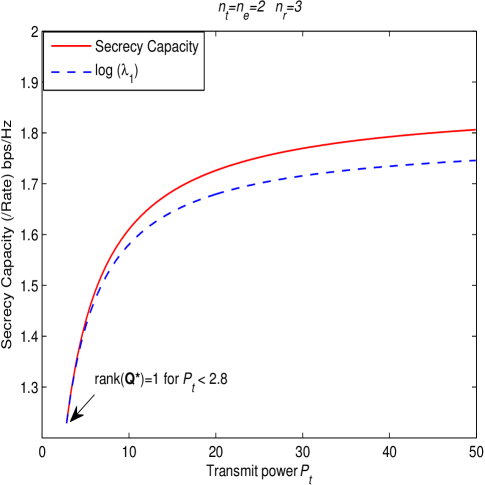
Figure 2: Secrecy Capacity versus $P_{t}$ for $n_{t}=n_{e}=2$ and $n_{r}=3$. Solid curve represents secrecy capacity and dotted curve indicates the achievable secrecy rate using a rank-one input covariance matrix.

In the first example, we consider a MIMO wiretap channel with $n_{t}=n_{e}=2$, $n_{t}=3$ and channel matrices given by

$${\mathbf{H}}=\left[\begin{array}[]{ccc}0.32-0.52i&0.83+1.15i\\ 0.51-0.26i&0.06-0.15i\\ -0.11+0.81i&0.29+0.68i\end{array}\right],$$ (82)

$${\mathbf{G}}=\left[\begin{array}[]{ccc}0.03-0.70i&-0.32-0.32i\\ 0.24-0.11i&1.36+0.18i\end{array}\right],$$ (85)

which satisfy ${\mathbf{H}}^{H}{\mathbf{H}}-{\mathbf{G}}^{H}{\mathbf{G}}\succ{\boldsymbol{0}}$. Fig. 2 shows the secrecy capacity as a function of transmit power $P_{t}$. For comparison, the figure also depicts the achievable secrecy rate using the input covariance matrix ${\mathbf{Q}}=P_{t}\,{\mathbf{u}}{\mathbf{u}}^{H}$, which results to $R_{sec}=\log\lambda_{1}$, as shown in [4]-[6]. Note that in this example, the optimal ${\mathbf{Q}}^{*}$ is not full-rank for $P_{t}<2.8$.

In Fig. 3 we consider another example of the case of ${\mathbf{H}}^{H}{\mathbf{H}}-{\mathbf{G}}^{H}{\mathbf{G}}\succ{\boldsymbol{0}}$, here with $n_{t}=n_{e}=3$, $n_{t}=4$ and channel matrices given by

$${\mathbf{H}}=\left[\begin{array}[]{ccc}0.89+0.54i&-0.06+0.60i&0.48-1.11i\\ 0.46&-0.44+0.80i&-1.07+0.63i\\ 1.40-0.13i&0.17-0.82i&0.59-0.31i\\ 0.43-0.23i&0.03+1.35i&0.44-0.07i\end{array}\right],$$ (90)

$${\mathbf{G}}=\left[\begin{array}[]{ccc}0.46-0.59i&0.24-0.01i&-0.37+0.15i\\ 0.51-0.63i&0.58+0.51i&0.86-0.47i\\ 0.17-0.24i&-0.83+0.51i&0.04-0.64i\end{array}\right].$$ (94)

For this example, the optimal ${\mathbf{Q}}^{*}$ is only full-rank for $P_{t}>0.5$.

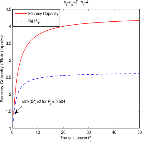
Figure 3: Secrecy Capacity versus $P_{t}$ for $n_{t}=n_{e}=3$ and $n_{r}=4$. Solid curve represents secrecy capacity and dotted curve indicates the achievable secrecy rate using a rank-one input covariance matrix.

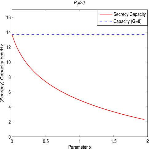
Figure 4: Secrecy Capacity versus $\alpha$ for $P_{t}=20$. Solid curve represents secrecy capacity and dashed curve indicates the point to point capacity.

Finally in Fig. 4, we compare the standard point-to-point capacity without secrecy constraints with the secrecy capacity given by (73). In this example, $P_{t}=20$, direct channel ${\mathbf{H}}$ is given by (90) but the cross channel ${\mathbf{G}}$ is assumed to satisfy ${\mathbf{G}}^{H}{\mathbf{G}}=\alpha{\mathbf{I}}$, where $\alpha$ changes from $0$ to $1.95$ (note that ${\mathbf{H}}^{H}{\mathbf{H}}-{\mathbf{G}}^{H}{\mathbf{G}}\succ{\boldsymbol{0}}$ only for $\alpha\leq 1.95$). As predicted, the secrecy capacity achieved by the derived ${\mathbf{Q}}^{*}$ in (71) approaches the standard capacity as ${\mathbf{G}}\rightarrow{\boldsymbol{0}}$. It is interesting to note that even for very small values of $\alpha$, the difference between the standard capacity and secrecy capacity is considerable.

VII Conclusion

In this paper, we considered the rank property of the optimal input covariance matrix under the average power constraint for a general MIMO Gaussian wiretap channel, where each node has an arbitrary number of antennas. We obtained necessary and sufficient constraints on the MIMO wiretap channel parameters such that the optimal input covariance matrix is full-rank, and we presented a method for characterizing the resulting covariance matrix as well.

Appendix A Proof of Lemma 4

Define $\bar{{\mathbf{S}}}=({\mathbf{H}}^{H}{\mathbf{H}}-{\mathbf{G}}^{H}{\mathbf{G}})^{-1}$ and apply the generalized eigenvalue decomposition on the pencil $(\bar{{\mathbf{S}}}^{\frac{1}{2}}{\mathbf{H}}^{H}{\mathbf{H}}\bar{{\mathbf{S}}}^{\frac{1}{2}}+{\mathbf{I}}\;,\;\bar{{\mathbf{S}}}^{\frac{1}{2}}{\mathbf{G}}^{H}{\mathbf{G}}\bar{{\mathbf{S}}}^{\frac{1}{2}}+{\mathbf{I}})$ to obtain the invertible generalized eigenvector matrix $\bar{{\mathbf{C}}}$ and the diagonal generalized eigenvalue matrix $\mathbf{\Lambda}_{\bar{{\mathbf{s}}}}$ as

$$\bar{{\mathbf{C}}}^{H}\left[\bar{{\mathbf{S}}}^{\frac{1}{2}}{\mathbf{H}}^{H}{\mathbf{H}}\bar{{\mathbf{S}}}^{\frac{1}{2}}+{\mathbf{I}}\right]\bar{{\mathbf{C}}} =\mathbf{\Lambda}_{\bar{{\mathbf{s}}}}$$ (95)

$$\bar{{\mathbf{C}}}^{H}\left[\bar{{\mathbf{S}}}^{\frac{1}{2}}{\mathbf{G}}^{H}{\mathbf{G}}\bar{{\mathbf{S}}}^{\frac{1}{2}}+{\mathbf{I}}\right]\bar{{\mathbf{C}}} ={\mathbf{I}}\;.$$ (96)

By subtracting (96) from (95), we have

$$\bar{{\mathbf{C}}}^{H}\,\bar{{\mathbf{C}}}=\mathbf{\Lambda}_{\bar{{\mathbf{s}}}}-{\mathbf{I}}\;.$$ (97)

Note that from Lemma 3, we have $\mathbf{\Lambda}_{\bar{{\mathbf{s}}}}-{\mathbf{I}}\succ{\boldsymbol{0}}$. Thus, $\bar{{\mathbf{C}}}$ must be of the form [14]

$$\bar{{\mathbf{C}}}={\mathbf{\Phi}}_{\bar{{\mathbf{s}}}}\,(\mathbf{\Lambda}_{\bar{{\mathbf{s}}}}-{\mathbf{I}})^{\frac{1}{2}}\;,$$ (98)

where ${\mathbf{\Phi}}_{\bar{{\mathbf{s}}}}$ is an unknown unitary matrix. In the following, as we continue the proof, ${\mathbf{\Phi}}_{\bar{{\mathbf{s}}}}$ is also characterized.

By replacing (98) in (95) and (96), it is revealed that the unitary matrix ${\mathbf{\Phi}}_{\bar{{\mathbf{s}}}}$ represents the common set of eigenvectors for the matrices $\bar{{\mathbf{S}}}^{\frac{1}{2}}{\mathbf{H}}^{H}{\mathbf{H}}\bar{{\mathbf{S}}}^{\frac{1}{2}}+{\mathbf{I}}$ and $\bar{{\mathbf{S}}}^{\frac{1}{2}}{\mathbf{G}}^{H}{\mathbf{G}}\bar{{\mathbf{S}}}^{\frac{1}{2}}+{\mathbf{I}}$, and thus both matrices commute. In particular,

$${\mathbf{\Phi}}_{\bar{{\mathbf{s}}}}^{H}\left[\bar{{\mathbf{S}}}^{\frac{1}{2}}{\mathbf{H}}^{H}{\mathbf{H}}\bar{{\mathbf{S}}}^{\frac{1}{2}}+{\mathbf{I}}\right]{\mathbf{\Phi}}_{\bar{{\mathbf{s}}}} =\mathbf{\Lambda}_{\bar{{\mathbf{s}}}}(\mathbf{\Lambda}_{\bar{{\mathbf{s}}}}-{\mathbf{I}})^{-1}={\mathbf{I}}+(\mathbf{\Lambda}_{\bar{{\mathbf{s}}}}-{\mathbf{I}})^{-1}$$ (99)

$${\mathbf{\Phi}}_{\bar{{\mathbf{s}}}}^{H}\left[\bar{{\mathbf{S}}}^{\frac{1}{2}}{\mathbf{G}}^{H}{\mathbf{G}}\bar{{\mathbf{S}}}^{\frac{1}{2}}+{\mathbf{I}}\right]{\mathbf{\Phi}}_{\bar{{\mathbf{s}}}} =(\mathbf{\Lambda}_{\bar{{\mathbf{s}}}}-{\mathbf{I}})^{-1}\;.$$ (100)

Defining ${\mathbf{D}}=(\mathbf{\Lambda}_{\bar{{\mathbf{s}}}}-{\mathbf{I}})^{-1}$, from (99)-(100) and via straightforward computation, we have

$${\mathbf{H}}^{H}{\mathbf{H}} =\bar{{\mathbf{S}}}^{-\frac{1}{2}}\,{\mathbf{\Phi}}_{\bar{{\mathbf{s}}}}\;{\mathbf{D}}\;{\mathbf{\Phi}}_{\bar{{\mathbf{s}}}}^{H}\bar{{\mathbf{S}}}^{-\frac{1}{2}}$$ (101)

$${\mathbf{G}}^{H}{\mathbf{G}} =\bar{{\mathbf{S}}}^{-\frac{1}{2}}\,{\mathbf{\Phi}}_{\bar{{\mathbf{s}}}}\;\left({\mathbf{D}}-{\mathbf{I}}\right)\;{\mathbf{\Phi}}_{\bar{{\mathbf{s}}}}^{H}\bar{{\mathbf{S}}}^{-\frac{1}{2}}\;,$$ (102)

which proves (53) and (54). Substituting (97) in (96), we also have

$${\mathbf{I}} =\bar{{\mathbf{C}}}^{H}\left[\bar{{\mathbf{S}}}^{\frac{1}{2}}{\mathbf{G}}^{H}{\mathbf{G}}\bar{{\mathbf{S}}}^{\frac{1}{2}}+{\mathbf{I}}\right]\bar{{\mathbf{C}}}$$

$$=\bar{{\mathbf{C}}}^{H}\bar{{\mathbf{S}}}^{\frac{1}{2}}{\mathbf{G}}^{H}{\mathbf{G}}\bar{{\mathbf{S}}}^{\frac{1}{2}}\bar{{\mathbf{C}}}+\mathbf{\Lambda}_{\bar{{\mathbf{s}}}}-{\mathbf{I}}\;,$$

or equivalently

$$2{\mathbf{I}}-\mathbf{\Lambda}_{\bar{{\mathbf{s}}}}=\bar{{\mathbf{C}}}^{H}\bar{{\mathbf{S}}}^{\frac{1}{2}}{\mathbf{G}}^{H}{\mathbf{G}}\bar{{\mathbf{S}}}^{\frac{1}{2}}\bar{{\mathbf{C}}}.$$

Remark 5.

Since $\bar{{\mathbf{C}}}^{H}\bar{{\mathbf{S}}}^{\frac{1}{2}}{\mathbf{G}}^{H}{\mathbf{G}}\bar{{\mathbf{S}}}^{\frac{1}{2}}\bar{{\mathbf{C}}}\succeq{\boldsymbol{0}}$, it results that $2{\mathbf{I}}-\mathbf{\Lambda}_{\bar{{\mathbf{s}}}}\succeq{\boldsymbol{0}}$. Equivalently, by defining ${\mathbf{D}}=(\mathbf{\Lambda}_{\bar{{\mathbf{s}}}}-{\mathbf{I}})^{-1}\succ{\boldsymbol{0}}$, we have

$$\begin{split}{\mathbf{I}}-{\mathbf{D}}^{-1}\succeq{\boldsymbol{0}}\\ {\mathbf{D}}-{\mathbf{I}}\succeq{\boldsymbol{0}}.\end{split}$$ (103)

Note that from (102), if ${\mathbf{G}}^{H}{\mathbf{G}}\succ{\boldsymbol{0}}$, then ${\mathbf{D}}-{\mathbf{I}}\succ{\boldsymbol{0}}$ and vice versa. As we will observe in Theorem 2, to have a full-rank optimal input covariance matrix ${\mathbf{Q}}^{*}$, having a full-rank ${\mathbf{G}}^{H}{\mathbf{G}}$ is not required. While we assume throughout the paper and without loss of generality that the diagonal matrix ${\mathbf{D}}-{\mathbf{I}}$ is invertible, for the case of rank deficient ${\mathbf{G}}^{H}{\mathbf{G}}$ one can follow the calculations in this paper assuming $\epsilon>0$ for zero-diagonal elements of ${\mathbf{D}}-{\mathbf{I}}$ and letting $\epsilon\downarrow 0$ at the end (see Lemma 7).

Appendix B Proof of Theorem 3

We want to obtain ${\mathbf{Q}}_{d}^{*}$, the optimal input covariance matrix that attains the secrecy capacity for the case of ${\mathbf{H}}^{H}{\mathbf{H}}-{\mathbf{G}}^{H}{\mathbf{G}}\succeq{\boldsymbol{0}}$. We note that $\mathrm{rank}({\mathbf{H}}^{H}{\mathbf{H}}-{\mathbf{G}}^{H}{\mathbf{G}})=m<n_{t}$. Hence, from Theorems 1 and 2, ${\mathbf{Q}}_{d}^{*}$ is rank-deficient.

The right hand side of (42) can be rewritten as

$$R({\mathbf{Q}}) =\log|{\mathbf{I}}+{\mathbf{H}}^{H}{\mathbf{H}}{\mathbf{Q}}|-\log|{\mathbf{I}}+{\mathbf{G}}^{H}{\mathbf{G}}{\mathbf{Q}}|$$

$$=\log|({\mathbf{I}}+{\mathbf{H}}^{H}{\mathbf{H}}{\mathbf{Q}})\,({\mathbf{I}}+{\mathbf{G}}^{H}{\mathbf{G}}{\mathbf{Q}})^{-1}|$$

$$=\log|{\mathbf{I}}+({\mathbf{H}}^{H}{\mathbf{H}}-{\mathbf{G}}^{H}{\mathbf{G}})\,{\mathbf{Q}}\,({\mathbf{I}}+{\mathbf{G}}^{H}{\mathbf{G}}{\mathbf{Q}})^{-1}|\;,$$ (104)

where Eq. (104) is obtained from the matrix inversion lemma [14] $({\mathbf{I}}+{\mathbf{A}})^{-1}={\mathbf{I}}-{\mathbf{A}}({\mathbf{I}}+{\mathbf{A}})^{-1}$. Let the eigenvalue decomposition of ${\mathbf{H}}^{H}{\mathbf{H}}-{\mathbf{G}}^{H}{\mathbf{G}}$ to be denoted as

$${\mathbf{H}}^{H}{\mathbf{H}}-{\mathbf{G}}^{H}{\mathbf{G}}={\mathbf{\Psi}}\left[\begin{array}[]{ccc}\mathbf{\Lambda}_{m}&{\boldsymbol{0}}\\ {\boldsymbol{0}}&{\boldsymbol{0}}\end{array}\right]{\mathbf{\Psi}}^{H}\;,$$ (107)

where $\mathbf{\Lambda}_{m}\succeq{\boldsymbol{0}}$ is a diagonal matrix of size $m\times m$. Using (107) in (104), we have

$$R({\mathbf{Q}}) =\log\left|{\mathbf{I}}+{\mathbf{\Psi}}\left[\begin{array}[]{ccc}\mathbf{\Lambda}_{m}&{\boldsymbol{0}}\\ {\boldsymbol{0}}&{\boldsymbol{0}}\end{array}\right]{\mathbf{\Psi}}^{H}\,{\mathbf{Q}}\,({\mathbf{I}}+{\mathbf{G}}^{H}{\mathbf{G}}{\mathbf{Q}})^{-1}\right|$$ (110)

$$=\log\left|{\mathbf{I}}+\left[\begin{array}[]{ccc}\mathbf{\Lambda}_{m}&{\boldsymbol{0}}\\ {\boldsymbol{0}}&{\boldsymbol{0}}\end{array}\right]{\mathbf{\Psi}}^{H}{\mathbf{Q}}{\mathbf{\Psi}}({\mathbf{I}}+{\mathbf{\Psi}}^{H}{\mathbf{G}}^{H}{\mathbf{G}}{\mathbf{\Psi}}\,{\mathbf{\Psi}}^{H}{\mathbf{Q}}{\mathbf{\Psi}})^{-1}\right|\;,$$ (113)

where in obtaining (113) we have used the facts that ${\mathbf{\Psi}}^{H}{\mathbf{\Psi}}={\mathbf{\Psi}}{\mathbf{\Psi}}^{H}={\mathbf{I}}$ and $|{\mathbf{I}}+{\mathbf{A}}{\mathbf{B}}|=|{\mathbf{I}}+{\mathbf{B}}{\mathbf{A}}|$.

Define $\bar{{\mathbf{Q}}}={\mathbf{\Psi}}^{H}{\mathbf{Q}}{\mathbf{\Psi}}$ and $\bar{{\mathbf{G}}}={\mathbf{G}}{\mathbf{\Psi}}$, so that the optimization problem in (42) can be rewritten as

$$\mathcal{C}_{sec}(P_{t})=\max_{\bar{{\mathbf{Q}}}\succeq{\boldsymbol{0}},\;\mathrm{Tr}(\bar{{\mathbf{Q}}})=P_{t}}\;R(\bar{{\mathbf{Q}}})\;,$$

where

$$R(\bar{{\mathbf{Q}}})=\log\left|{\mathbf{I}}+\left[\begin{array}[]{ccc}\mathbf{\Lambda}_{m}&{\boldsymbol{0}}\\ {\boldsymbol{0}}&{\boldsymbol{0}}\end{array}\right]\bar{{\mathbf{Q}}}\,({\mathbf{I}}+\bar{{\mathbf{G}}}^{H}\bar{{\mathbf{G}}}\,\bar{{\mathbf{Q}}})^{-1}\right|.$$ (116)

From right-hand side of (116), we see that the optimal $\bar{{\mathbf{Q}}}$ is of the form

$$\bar{{\mathbf{Q}}}=\left[\begin{array}[]{ccc}\bar{{\mathbf{Q}}}_{m}&{\boldsymbol{0}}\\ {\boldsymbol{0}}&{\boldsymbol{0}}\end{array}\right]\;,$$ (119)

where $\bar{{\mathbf{Q}}}_{m}\succeq{\boldsymbol{0}}$ is of size $m\times m$. Write $\bar{{\mathbf{G}}}^{H}\bar{{\mathbf{G}}}$ as

$$\bar{{\mathbf{G}}}^{H}\bar{{\mathbf{G}}}=\left[\begin{array}[]{ccc}{\mathbf{J}}_{1}&{\mathbf{J}}_{2}\\ {\mathbf{J}}_{2}^{H}&{\mathbf{J}}_{3}\end{array}\right]$$ (122)

where ${\mathbf{J}}_{1}$, ${\mathbf{J}}_{2}$ and ${\mathbf{J}}_{3}$ are of dimensions $m\times m$, $m\times(n_{t}-m)$ and $(n_{t}-m)\times(n_{t}-m)$, respectively. By substituting (119) and (122) into (116), we obtain

$$R(\bar{{\mathbf{Q}}}) =\log\left|{\mathbf{I}}+\left[\begin{array}[]{ccc}\mathbf{\Lambda}_{m}\bar{{\mathbf{Q}}}_{m}&{\boldsymbol{0}}\\ {\boldsymbol{0}}&{\boldsymbol{0}}\end{array}\right]\left[\begin{array}[]{ccc}{\mathbf{I}}+{\mathbf{J}}_{1}\bar{{\mathbf{Q}}}_{m}&{\boldsymbol{0}}\\ {\mathbf{J}}_{2}^{H}\bar{{\mathbf{Q}}}_{m}&{\mathbf{I}}\end{array}\right]^{-1}\right|$$ (127)

$$=\log\left|{\mathbf{I}}+\left[\begin{array}[]{ccc}\mathbf{\Lambda}_{m}\bar{{\mathbf{Q}}}_{m}&{\boldsymbol{0}}\\ {\boldsymbol{0}}&{\boldsymbol{0}}\end{array}\right]\left[\begin{array}[]{ccc}({\mathbf{I}}+{\mathbf{J}}_{1}\bar{{\mathbf{Q}}}_{m})^{-1}&{\boldsymbol{0}}\\ -{\mathbf{J}}_{2}^{H}\bar{{\mathbf{Q}}}_{m}({\mathbf{I}}+{\mathbf{J}}_{1}\bar{{\mathbf{Q}}}_{m})^{-1}&{\mathbf{I}}\end{array}\right]\right|$$ (132)

$$=\log\left|{\mathbf{I}}+\left[\begin{array}[]{ccc}\mathbf{\Lambda}_{m}\bar{{\mathbf{Q}}}_{m}({\mathbf{I}}+{\mathbf{J}}_{1}\bar{{\mathbf{Q}}}_{m})^{-1}&{\boldsymbol{0}}\\ {\boldsymbol{0}}&{\boldsymbol{0}}\end{array}\right]\right|$$ (135)

$$=\log\left|\left[\begin{array}[]{ccc}{\mathbf{I}}+\mathbf{\Lambda}_{m}\bar{{\mathbf{Q}}}_{m}({\mathbf{I}}+{\mathbf{J}}_{1}\bar{{\mathbf{Q}}}_{m})^{-1}&{\boldsymbol{0}}\\ {\boldsymbol{0}}&{\mathbf{I}}\end{array}\right]\right|$$ (138)

$$=\log\left|{\mathbf{I}}+\mathbf{\Lambda}_{m}\bar{{\mathbf{Q}}}_{m}({\mathbf{I}}+{\mathbf{J}}_{1}\bar{{\mathbf{Q}}}_{m})^{-1}\right|$$

$$=\log\left|{\mathbf{I}}+(\mathbf{\Lambda}_{m}+{\mathbf{J}}_{1})\bar{{\mathbf{Q}}}_{m}\right|-\log\left|{\mathbf{I}}+{\mathbf{J}}_{1}\bar{{\mathbf{Q}}}_{m}\right|=R(\bar{{\mathbf{Q}}}_{m}).$$ (139)

Using (127), the secrecy capacity is given by

$$\mathcal{C}_{sec}(P_{t})=\max_{\bar{{\mathbf{Q}}}_{m}\succeq{\boldsymbol{0}},\;\mathrm{Tr}(\bar{{\mathbf{Q}}}_{m})=P_{t}}\;R(\bar{{\mathbf{Q}}}_{m})\;.$$ (140)

Problem (140) shows that the secrecy capacity of a wiretap channel with ${\mathbf{H}}^{H}{\mathbf{H}}-{\mathbf{G}}^{H}{\mathbf{G}}\succeq{\boldsymbol{0}}$ is equal to the secrecy capacity of an equivalent wiretap channel with

$${\mathbf{H}}_{eq}^{H}{\mathbf{H}}_{eq} =\mathbf{\Lambda}_{m}+{\mathbf{J}}_{1}$$ (141)

$${\mathbf{G}}_{eq}^{H}{\mathbf{G}}_{eq} ={\mathbf{J}}_{1}\;,$$ (142)

where $\mathbf{\Lambda}_{m}$ and ${\mathbf{J}}_{1}$ are respectively given by (107) and (122). It should also be noted that for the equivalent channel, ${\mathbf{H}}_{eq}^{H}{\mathbf{H}}_{eq}-{\mathbf{G}}_{eq}^{H}{\mathbf{G}}_{eq}=\mathbf{\Lambda}_{m}\succ{\boldsymbol{0}}$. Thus, the optimal $\bar{{\mathbf{Q}}}_{m}^{*}$ can be computed using Theorem 2, as long as the equivalent channel satisfies the second condition in Theorem 2. Finally, by substituting $\bar{{\mathbf{Q}}}_{m}^{*}$ back into (119) we obtain

$${\mathbf{Q}}_{d}^{*}={\mathbf{\Psi}}\left[\begin{array}[]{ccc}\bar{{\mathbf{Q}}}^{*}_{m}&{\boldsymbol{0}}\\ {\boldsymbol{0}}&{\boldsymbol{0}}\end{array}\right]{\mathbf{\Psi}}^{H}\,,$$ (145)

which completes the proof.

References

[1]
A. Wyner, “The wire-tap channel,” Bell. Syst. Tech. J., vol. 54, no. 8, pp. 1355-1387, Jan. 1975.
[2]
S. K. Leung-Yan-Cheong and M. E. Hellman, “The Gaussian wire-tap channel,” IEEE Trans. Inf. Theory, vol. 24, pp. 451-456, Jul. 1978.
[3]
F. Oggier and B. Hassibi, “The secrecy capacity of the MIMO wiretap channel,” in Proc. IEEE Int. Symp. Information Theory Toronto, ON, Canada, Jul. 2008, pp. 524-528.
[4]
A. Khisti and G. Wornell, “Secure transmission with multiple antennas II: The MIMOME
wiretap channel,” IEEE Trans. Inf. Theory, vol. 56, no. 11, pp. 5515-5532, 2010.
[5]
J. Li and A. P. Petropulu, “Transmitter optimization for achieving secrecy capacity in Gaussian MIMO wiretap channels,”
submitted to IEEE Trans. Info. Theory, Available [online]: http://arxiv.org/PS cache/arxiv/pdf/0909/0909.2622v1.pdf.
[6]
A. Khisti and G. Wornell, “Secure transmission with multiple antennas I: The MISOME
wiretap channel,” IEEE Trans. Inf. Theory, vol. 56, no. 7, pp. 3088-3104, 2010.
[7]
S. Shafiee and S. Ulukus, “Towards the Secrecy Capacity of the Gaussian MIMO
Wire-Tap Channel: The 2-2-1 Channel,” IEEE Trans. on Inf. Theory, vol. 55, no. 9, Sep. 2009.
[8]
T. Liu and S. Shamai (Shitz), “A note on secrecy capacity of the multi-antenna wiretap channel,” IEEE Trans. Inf. Theory, vol. 55, no. 6, pp. 2547-2553, 2009.
[9]
R. Bustin, R. Liu, H. V. Poor, and S. Shamai (Shitz), “A MMSE approach to the secrecy capacity of the MIMO Gaussian wiretap channel,” EURASIP Journal on Wireless Communications and Networking, vol. 2009, Article ID 370970, 8 pages, 2009.
[10]
H. Weingarten, Y. Steinberg, and S. Shamai (Shitz), “The capacity region of the Gaussian multiple-input multipleoutput broadcast channel,” IEEE Trans. Inf. Theory, vol. 52, no. 9, pp. 3936-3964, 2006.
[11]
R. Liu, I. Maric, P. Spasojevic, and R. D. Yates, “Discrete memoryless interference and broadcast
channels with confidential messages: Secrecy rate regions,” IEEE Trans. Inf. Theory, vol. 54, no. 6, pp. 2493-2512, June 2008.
[12]
R. Liu and H. V. Poor, “Secrecy capacity region of a multiple-antenna Gaussian broadcast channel with confidential messages,” IEEE Trans. Inf. Theory, vol. 55, no. 3, pp. 1235-1249, Mar. 2009.
[13]
R. Liu, T. Liu, H. V. Poor, and S. Shamai, “Multiple-input multiple-output Gaussian broadcast channels with confidential messages,” IEEE Trans. Inf. Theory, vol. 56, no. 9, pp. 4215-4227, 2010.
[14]
R. A. Horn and C. R. Johnson, Matrix Analysis, University Press, Cambridge, UK, 1999.
[15]
C. F. V. Loan, “Generalizing the Singular Value Decomposition,” SIAM Journal on Num. Analysis, vol. 13, no. 1, pp. 76-83, Mar. 1973.