A Topological Introduction to Knot Contact Homology

Abstract.

This is a survey of knot contact homology, with an emphasis on topological, algebraic, and combinatorial aspects.

1. Introduction

This article is intended to serve as a general introduction to the subject of knot contact homology. There are two related sides to the theory: a geometric side devoted to the contact geometry of conormal bundles and explicit calculation of holomorphic curves, and an algebraic, combinatorial side emphasizing ties to knot theory and topology. We will focus on the latter side and only treat the former side lightly. The present notes grew out of lectures given at the Contact and Symplectic Topology Summer School in Budapest in July 2012.

The strategy of studying the smooth topology of a smooth manifold via the symplectic topology of its cotangent bundle is an idea that was advocated by V. I. Arnold and has been extensively studied in symplectic geometry in recent years. It is well-known that if $M$ is smooth then $T^{*}M$ carries a natural symplectic structure, with symplectic form $\omega=-d\lambda_{\text{can}}$, where $\lambda_{\text{can}}\in\Omega^{1}(T^{*}M)$ is the Liouville form; the idea then is to analyze $T^{*}M$ as a symplectic manifold to recover topological data about $M$.

In recent years this strategy has been executed quite successfully by examining Gromov-type moduli spaces of holomorphic curves on $T^{*}M$. For instance, one can show that the symplectic structure on $T^{*}M$ recovers homotopic information about $M$, as shown in various guises by Viterbo [Vit], Salamon–Weber [SW06], and Abbondandolo–Schwarz [AS06], who each prove some version of the following result (where technical restrictions have been omitted for simplicity):

Theorem 1.1 ([Vit, SW06, AS06]).

The Hamiltonian Floer homology of $T^{*}M$ is isomorphic to the singular homology of the free loop space of $M$.

Subsequent work has related certain additional Floer-theoretic constructions on $T^{*}M$ to the Chas–Sullivan loop product and string topology; see for example [AS10, CL09].

In a slightly different direction, M. Abouzaid has used holomorphic curves to show that the symplectic structure on $T^{*}M$ can contain more than topological information about $M$:

Theorem 1.2 ([Abo12]).

If $\Sigma$ is an exotic $(4k+1)$-sphere that does not bound a parallelizable manifold, then $T^{*}\Sigma$ is not symplectomorphic to $T^{*}S^{4k+1}$.

At the time of this writing, it is still possible that the smooth type of a closed smooth manifold $M$ (up to diffeomorphism) is determined by the symplectic type of $T^{*}M$ (up to symplectomorphism), which would be a very strong endorsement of Arnold’s idea. (See however [Kna] for counterexamples when $M$ is not closed.) For a nice discussion of this and related problems, see [Per10].

In this survey article, we discuss a relative version of Arnold’s strategy. The setting is as follows. Let $K\subset M$ be an embedded submanifold (or an immersed submanifold with transverse self-intersections). Then one can construct the conormal bundle of $K$:

$$L_{K}=\{(q,p)\,|\,q\in K,~{}\langle p,v\rangle=0\text{ for all }v\in T_{q}K\}\subset T^{*}M.$$

It is a standard exercise to check that $L_{K}$ is a Lagrangian submanifold of $T^{*}M$.

One can work in one dimension lower by considering the cosphere (unit cotangent) bundle $ST^{*}M$ of unit covectors in $T^{*}M$ with respect to some metric; then $ST^{*}M$ is a contact manifold with contact form $\alpha=\lambda_{\text{can}}$, and it can be shown that the contact structure on $ST^{*}M$ is independent of the metric. The unit conormal bundle of $K$,

$$\Lambda_{K}=L_{K}\cap ST^{*}M\subset ST^{*}M,$$

is then a Legendrian submanifold of $ST^{*}M$, with $\alpha|_{\Lambda_{K}}=0$. See Figure 1.

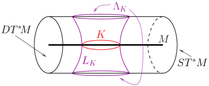
Figure 1. A schematic depiction of cotangent and conormal bundles. Only the disk bundle portion $DT^{*}M$ of $T^{*}M$ is shown, with boundary $ST^{*}M$. Note that both $L_{K}$ and the zero section $M$ are Lagrangian in $T^{*}M$, and their intersection is $K$.

By construction, if $K$ changes by smooth isotopy in $M$, then $\Lambda_{K}$ changes by Legendrian isotopy (isotopy within the class of Legendrian submanifolds) in $ST^{*}M$. One can then ask what the Legendrian isotopy type of $\Lambda_{K}$ remembers about the smooth isotopy type of $K$; see Question 1.3 below.

For the remainder of the section and article, we restrict our focus by assuming that $M=\mathbb{R}^{3}$ and $K\subset\mathbb{R}^{3}$ is a knot or link. In this case, $ST^{*}M$ is contactomorphic to the $1$-jet space $J^{1}(S^{2})=T^{*}S^{2}\times\mathbb{R}$ equipped with the contact form $dz-\lambda_{\text{can}}$, where $z$ is the coordinate on $\mathbb{R}$ and $\lambda_{\text{can}}$ is the Liouville form on $S^{2}$, via the diffeomorphism $ST^{*}\mathbb{R}^{3}\to J^{1}(S^{2})$ sending $(q,p)$ to $((p,q-\langle q,p\rangle p),\langle q,p\rangle)$ where $\langle\cdot,\cdot\rangle$ is the standard metric on $\mathbb{R}^{3}$.

In the $5$-manifold $ST^{*}\mathbb{R}^{3}$, the unit conormal bundle $\Lambda_{K}$ is topologically a $2$-torus (or a disjoint union of tori if $K$ has multiple components). This can for instance be seen in the dual picture in $TR^{3}$, where the unit normal bundle can be viewed as the boundary of a tubular neighborhood of $K$. The topological type of $\Lambda_{K}\cong T^{2}\subset S^{2}\times\mathbb{R}^{3}$ contains no information: if $K_{1},K_{2}$ are arbitrary knots, then $\Lambda_{K_{1}}$ and $\Lambda_{K_{2}}$ are smoothly isotopic. (Choose a one-parameter family of possibly singular knots $K_{t}$ joining $K_{1}$ to $K_{2}$, and perturb $\Lambda_{K_{t}}$ slightly when $K_{t}$ is singular to eliminate double points.)

However, there is no reason for $\Lambda_{K_{1}}$ and $\Lambda_{K_{2}}$ to be Legendrian isotopic. This suggests the following question.

Question 1.3.

How much of the topology of $K\subset\mathbb{R}^{3}$ is encoded in the Legendrian structure of $\Lambda_{K}\subset ST^{*}\mathbb{R}^{3}$? If $\Lambda_{K_{1}}$ and $\Lambda_{K_{2}}$ are Legendrian isotopic, are $K_{1}$ and $K_{2}$ necessarily smoothly isotopic knots?

At the present, the answer to the second part of this question is unknown but could possibly be “yes”. The answer is known to be “yes” if either knot is the unknot; see below.

In order to tackle Question 1.3, it is useful to have invariants of Legendrian submanifolds under Legendrian isotopy. One particularly powerful invariant is Legendrian contact homology, which is a Floer-theoretic count of holomorphic curves associated to a Legendrian submanifold and is discussed in more detail in Section 2.

Definition 1.4.

Let $K\subset\mathbb{R}^{3}$ be a knot or link. The knot contact homology of $K$, written $HC_{*}(K)$, is the Legendrian contact homology of $\Lambda_{K}$.

Knot contact homology is the homology of a differential graded algebra associated to a knot, the knot DGA $(\mathcal{A},\partial)$. By the general invariance result for Legendrian contact homology, the knot DGA and knot contact homology are topological invariants of knots and links.

This article is a discussion of knot contact homology and its properties. Despite the fact that the original definition of knot contact homology involves holomorphic curves, there is a purely combinatorial formulation of knot contact homology. The article [EENS13b], which does most of the heavy lifting for the results presented here, derives this combinatorial formula and can be viewed as the first reasonably involved computation of Legendrian contact homology in high dimensions.

Viewed from a purely knot theoretic perspective, knot contact homology is a reasonably strong knot invariant. For instance, it detects the unknot (see Corollaries 4.10 and 5.10): if $K$ is a knot such that $HC_{*}(K)\cong HC_{*}(O)$ where $O$ is the unknot, then $K=O$. This implies in particular that the answer to Question 1.3 is yes if one of the knots is unknotted. It is currently an open question whether knot contact homology is a complete knot invariant.

Connections between knot contact homology and other knot invariants are gradually beginning to appear. It is known that $HC_{*}(K)$ determines the Alexander polynomial (Theorem 3.18). A portion of the homology also has a natural topological interpretation, via an object called the cord algebra that is closely related to string topology. In addition, one can use $HC_{*}(K)$ to define a three-variable knot invariant, the augmentation polynomial, which is closely related to the $A$-polynomial and conjecturally determines a specialization of the HOMFLY-PT polynomial. Very recently, a connection between knot contact homology and string theory has been discovered, and this suggests that the augmentation polynomial may in fact determine many known knot invariants, including the HOMFLY-PT polynomial and certain knot homologies, and may also be determined by a recursion relation for colored HOMFLY-PT polynomials.

Knot contact homology also produces a strong invariant of transverse knots, which are knots that are transverse to the standard contact structure on $\mathbb{R}^{3}$. For a transverse knot, the knot contact homology of the underlying topological knot contains an additional filtered structure, transverse homology, which is invariant under transverse isotopy. This has been shown to be an effective transverse invariant (Theorem 6.9), one of two that are currently known (the other comes from Heegaard Floer theory).

Figure 2. The knot invariants and interconnections described in this article.

In the rest of the article, we expand on the properties of knot contact homology mentioned above; see Figure 2 for a schematic chart. In Section 2, we review the general definition of Legendrian contact homology. We apply this to knots and conormal bundles in Section 3 to give a combinatorial definition of knot contact homology and present a few of its properties. In Section 4, we discuss the cord algebra, which gives a topological interpretation of knot contact homology in degree $0$. Section 5 defines the augmentation polynomial and relates it to other knot invariants; this includes a speculative discussion of the relation to string theory. In Section 6, we present transverse homology and consider its effectiveness as an invariant of transverse knots. Some technical details (a definition of the “fully noncommutative” version of knot contact homology, and a comparison of the conventions used in this article to conventions in the literature) are included in the Appendix.

As this is a survey article, many details will be omitted in favor of what we hope is an accessible exposition of the subject. (For more introductory material on knot contact homology, the reader is referred to two papers [EE05, Ng06]; note however that these do not contain recent developments.) There are exercises scattered through the text as a concrete, hands-on complement to the main discussion. There is not much new mathematical content in this article beyond what has already appeared in the literature, particularly [EENS13a, EENS13b] on the geometric side and [Ng05a, Ng05b, Ng08, Ng11] on the combinatorial/topological side. One exception is a representation-theoretic interpretation of some factors of the augmentation polynomial that do not appear in the $A$-polynomial; see Theorem 5.11. We have also introduced a number of conventions for combinatorial knot contact homology in this article that are new and, in the author’s opinion, more natural than previous conventions.

Acknowledgments

I am grateful to the organizers and participants of the 2012 Contact and Symplectic Topology Summer School in Budapest, and particularly Chris Cornwell and Tobias Ekholm, for a great deal of helpful feedback, and to Dan Rutherford for catching a typo in an earlier draft. This work was partially supported by NSF CAREER grant DMS-0846346.

2. Legendrian Contact Homology

In this section, we give a cursory introduction to Legendrian contact homology and augmentations, essentially the minimum necessary to motivate the construction of knot contact homology in Section 3. The reader interested in further details is referred to the various references given in this section.

Legendrian contact homology (LCH), introduced by Eliashberg and Hofer in [Eli98], is an invariant of Legendrian submanifolds in suitable contact manifolds. This invariant is defined by counting certain holomorphic curves in the symplectization of the contact manifold, and is a part of the (much larger) Symplectic Field Theory package of Eliashberg, Givental, and Hofer [EGH00]. LCH is the homology of a differential graded algebra (DGA) that we now describe, and in some sense the DGA (up to an appropriate equivalence relation), rather than the homology, is the “true” invariant of the Legendrian submanifold.

In this section, we will work exclusively in a contact manifold of the form $V=J^{1}(M)=T^{*}M\times\mathbb{R}$ with the standard contact form $\alpha=dz-\lambda_{\text{can}}$. LCH can be defined for much more general contact manifolds, but the proof of invariance in general has not been fully carried out, and even the definition is more complicated than the one given below when the contact manifold has closed Reeb orbits. Note that for $V=J^{1}(M)$, the Reeb vector field $R_{\alpha}$ is $\partial/\partial z$ and thus $J^{1}(M)$ has no closed Reeb orbits.

Let $\Lambda\subset V$ be a Legendrian submanifold. We assume for simplicity that $\Lambda$ has trivial Maslov class (e.g., for Legendrian knots in $\mathbb{R}^{3}=J^{1}(\mathbb{R})$, this means that $\Lambda$ has rotation number $0$), and that $\Lambda$ has finitely many Reeb chords, integral curves for the Reeb field $R_{\alpha}$ with endpoints on $\Lambda$. We label the Reeb chords formally as $a_{1},\ldots,a_{n}$. Finally, let $R$ denote (here and throughout the article) the coefficient ring $R=\mathbb{Z}[H_{2}(V,\Lambda)]$, the group ring of the relative homology group $H_{2}(V,\Lambda)$.

Definition 2.1.

The LCH differential graded algebra associated to $\Lambda$ is $(\mathcal{A},\partial)$, defined as follows:

1. Algebra: $\mathcal{A}=R\langle a_{1},\ldots,a_{n}\rangle$ is the free noncommutative unital algebra over $R$ generated by $a_{1},\ldots,a_{n}$. As an $R$-module, $\mathcal{A}$ is generated by all words $a_{i_{1}}\cdots a_{i_{k}}$ for $k\geq 0$ (where $k=0$ gives the empty word $1$).

2. Grading: Define $|a_{i}|=CZ(a_{i})-1$, where $CZ$ denotes Conley–Zehnder index (see [EES07] for the definition in this context) and $|r|=0$ for $r\in R$. Extend the grading to all of $\mathcal{A}$ in the usual way: $|xy|=|x|+|y|$.

3. Differential: Define $\partial(r)=0$ for $r\in R$ and

   $$\partial(a_{i})=\sum_{\dim\mathcal{M}(a_{i};a_{j_{1}},\ldots,a_{j_{k}})/\mathbb{R}=0}~{}~{}\sum_{\Delta\in\mathcal{M}/\mathbb{R}}(\textrm{sgn}(\Delta))e^{[\Delta]}a_{j_{1}}\cdots a_{j_{k}}$$

   where $\mathcal{M}(a_{i};a_{j_{1}},\ldots,a_{j_{k}})$ is the moduli space defined below, $\text{sgn}(\Delta)$ is an orientation sign associated to $\Delta$, and $[\Delta]$ is the homology class of $\Delta$ in $H_{2}(V,\Lambda)$.

   Extend the differential to all of $\mathcal{A}$ via the signed Leibniz rule: $\partial(xy)=(\partial x)y+(-1)^{|x|}x(\partial y)$.

The key to Definition 2.1 is the moduli space $\mathcal{M}(a_{i};a_{j_{1}},\ldots,a_{j_{k}})$. To define this, let $J$ be a (suitably generic) almost complex structure on the symplectization $(\mathbb{R}\times V,d(e^{t}\alpha))$ of $V$ (where $\alpha$ is the contact form on $V$ and $t$ is the $\mathbb{R}$ coordinate) that is compatible with the symplectization in the following sense: $J$ is $\mathbb{R}$-invariant, $J(\partial/\partial t)=R_{\alpha}$, and $J$ maps $\xi=\ker\alpha$ to itself. With respect to this almost complex structure, $\mathbb{R}\times a_{i}$ is a holomorphic strip for any Reeb chord $a_{i}$ of $\Lambda$.

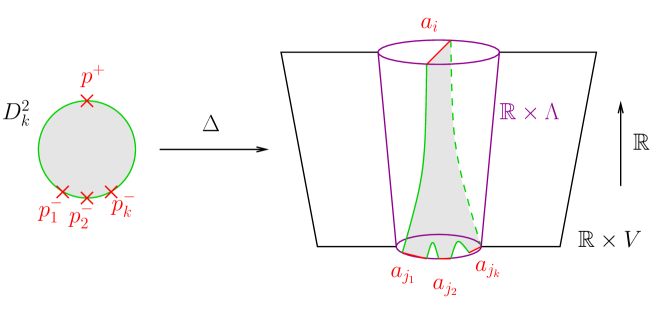
Figure 3. A holomorphic disk $\Delta:\thinspace(D^{2}_{k},\partial D^{2}_{k})\to(\mathbb{R}\times V,\mathbb{R}\times\Lambda)$ contributing to $\mathcal{M}(a_{i};a_{j_{1},\ldots,a_{j_{k}}})$ and the differential $\partial(a_{i})$.

Let $D^{2}_{k}=D^{2}\setminus\{p^{+},p_{1}^{-},\ldots,p_{k}^{-}\}$ be a closed disk with $k+1$ punctures on its boundary, labeled $p^{+},p_{1}^{-},\ldots,p_{k}^{-}$ in counterclockwise order around $\partial D^{2}$. For (not necessarily distinct) Reeb chords $a_{i}$ and $a_{j_{1}},\ldots,a_{j_{k}}$ for some $k\geq 0$, let $\mathcal{M}(a_{i};a_{j_{1}},\ldots,a_{j_{k}})$ be the moduli space of $J$-holomorphic maps

$$\Delta:\thinspace(D^{2}_{k},\partial D^{2}_{k})\to(\mathbb{R}\times V,\mathbb{R}\times\Lambda)$$

up to domain reparametrization, such that:

• near $p^{+}$, $\Delta$ is asymptotic to a neighborhood of the Reeb strip $\mathbb{R}\times a_{i}$ near $t=+\infty$;

• near $p_{l}^{-}$ for $1\leq l\leq k$, $\Delta$ is asymptotic to a neighborhood of $\mathbb{R}\times a_{j_{l}}$ near $t=-\infty$.

See Figure 3.

When everything is suitably generic, $\mathcal{M}(a_{i};a_{j_{1}},\ldots,a_{j_{k}})$ is a manifold of dimension $|a_{i}|-\sum_{l}|a_{j_{l}}|$. The moduli space also has an $\mathbb{R}$ action given by translation in the $\mathbb{R}$ direction, and the differential $\partial(a_{i})$ counts moduli spaces $\mathcal{M}(a_{i};a_{j_{1}},\ldots,a_{j_{k}})$ that are rigid after quotienting by this $\mathbb{R}$ action.

Remark 2.2.

If $H_{2}(V,\Lambda)\cong H_{2}(V)\oplus H_{1}(\Lambda)$, as is true in the case that we will consider, one can “improve” the DGA $(\mathcal{A},\partial)$ to a DGA that we might call the fully noncommutative DGA $(\widetilde{\mathcal{A}},\partial)$, defined as follows. For simplicity, assume that $\Lambda$ is connected; there is a similar but slightly more involved construction otherwise. The algebra $\widetilde{\mathcal{A}}$ is the tensor algebra over the group ring $\mathbb{Z}[H_{2}(V)]$, generated by the Reeb chords $a_{1},\ldots,a_{n}$ along with elements of $\pi_{1}(\Lambda)$, with no relations except for the ones inherited from $\pi_{1}(\Lambda)$. Thus $\widetilde{\mathcal{A}}$ is generated as a $\mathbb{Z}[H_{2}(V)]$-module by words of the form

$$\gamma_{0}a_{i_{1}}\gamma_{1}a_{i_{2}}\gamma_{2}\cdots\gamma_{k-1}a_{i_{k}}\gamma_{k}$$

where $a_{i_{1}},\ldots,a_{i_{k}}$ are Reeb chords of $\Lambda$, $\gamma_{0},\ldots,\gamma_{k}\in\pi_{1}(\Lambda)$, and $k\geq 0$. Note that $\mathcal{A}$ is a quotient of $\widetilde{\mathcal{A}}$: just abelianize $\pi_{1}(\Lambda)$ to $H_{1}(\Lambda)$, and allow Reeb chords $a_{i}$ to commute with homology classes $\gamma\in H_{1}(\Lambda)$.

To define the differential, let $\Delta$ be a disk in $\mathcal{M}(a_{i};a_{j_{1}},\ldots,a_{j_{k}})$. The projection map $\pi:\thinspace H_{2}(V,\Lambda)\to H_{2}(V)$ gives a class $\pi([\Delta])\in H_{2}(V)$. The boundary of the image of $\Delta$ consists of an ordered collection of $k+1$ paths in $\Lambda$ joining endpoints of Reeb chords. By fixing paths in $\Lambda$ joining each Reeb chord endpoint to a fixed point on $\Lambda$, one can close these $k+1$ paths into $k+1$ loops in $\Lambda$. Let $\gamma_{0}(\Delta),\ldots,\gamma_{k}(\Delta)$ denote the homotopy classes of these loops in $\pi_{1}(\Lambda)$, where the loops are ordered in the order that they appear in the image of $\partial D^{2}$, traversed counterclockwise. Finally, define $\partial(\gamma)=0$ for $\gamma\in\pi_{1}(\Lambda)$ and

$$\partial(a_{i})=\sum_{\dim\mathcal{M}(a_{i};a_{j_{1}},\ldots,a_{j_{k}})/\mathbb{R}=0}~{}~{}\sum_{\Delta\in\mathcal{M}/\mathbb{R}}(\textrm{sgn}(\Delta))e^{\pi([\Delta])}\gamma_{0}(\Delta)a_{j_{1}}\gamma_{1}(\Delta)\cdots a_{j_{k}}\gamma_{k}(\Delta),$$

and extend the differential to $\widetilde{\mathcal{A}}$ by the Leibniz rule.

Note that the quotient that sends $\widetilde{\mathcal{A}}$ to $\mathcal{A}$ also sends the differential on $\widetilde{\mathcal{A}}$ to the differential on $\mathcal{A}$. The fully noncommutative DGA $(\widetilde{\mathcal{A}},\partial)$ satisfies the same properties as $(\mathcal{A},\partial)$ (Theorem 2.3 below), with a suitable alteration of the definition of stable tame isomorphism. For the majority of this article, we will stick to the usual LCH DGA $(\mathcal{A},\partial)$, which is enough for most purposes, because it simplifies notation; see however the discussion after Theorem 4.8, as well as the Appendix.

We now state some fundamental properties of the LCH DGA $(\mathcal{A},\partial)$. These began with the work of Eliashberg–Hofer [Eli98]; Chekanov [Che02] wrote down the precise statement and gave a combinatorial proof for the case $V=\mathbb{R}^{3}$ (see also [ENS02]). The formulation given here is due to, and proven by, Ekholm–Etnyre–Sullivan [EES07].

Theorem 2.3 ([Eli98, Che02, EES07]).

Given suitable genericity assumptions:

1. $\partial$ decreases degree by 1;

2. $\partial^{2}=0$;

3. up to stable tame isomorphism, $(\mathcal{A},\partial)$ is independent of all choices (of contact form for the contact structure on $V$, and of $J$), and is an invariant of $\Lambda$ up to Legendrian isotopy;

4. up to isomorphism, $H_{*}(\mathcal{A},\partial)=:HC_{*}(V,\Lambda)$ is also an invariant of $\Lambda$ up to Legendrian isotopy.

Here “stable tame isomorphism” is an equivalence relation between DGAs defined in Definition 2.4 below, which is a special case of quasi-isomorphism; thus item 3 in Theorem 2.3 directly implies item 4. The homology $HC_{*}(V,\Lambda)$ is called the Legendrian contact homology of $\Lambda$.

Definition 2.4 ([Che02], see also [ENS02]).

1. Let $\mathcal{A}=R\langle a_{1},\ldots,a_{n}\rangle$. An elementary automorphism of $\mathcal{A}$ is an algebra map $\phi:\thinspace\mathcal{A}\to\mathcal{A}$ of the form: for some $i$, $\phi(a_{j})=a_{j}$ for all $j\neq i$, and $\phi(a_{i})=a_{i}+v$ for some $v\in R\langle a_{1},\ldots,a_{i-1},a_{i+1},\ldots,a_{n}\rangle$.

2. A tame automorphism of $\mathcal{A}$ is a composition of elementary automorphisms.

3. DGAs $(\mathcal{A}=R\langle a_{1},\ldots,a_{n}\rangle,\partial)$ and $(\mathcal{A}^{\prime}=R\langle a_{1}^{\prime},\ldots,a_{n}^{\prime}\rangle,\partial^{\prime})$ are tamely isomorphic if there is an algebra isomorphism $\psi=\phi_{2}\circ\phi_{1}$ such that $\phi_{1}:\thinspace\mathcal{A}\to\mathcal{A}$ is a tame automorphism and $\phi_{2}:\thinspace\mathcal{A}\to\mathcal{A}^{\prime}$ is given by $\phi_{2}(a_{i})=a_{i}^{\prime}$ for all $i$, and $\psi$ intertwines the differentials: $\psi\circ\partial=\partial^{\prime}\circ\psi$.

4. A stabilization of $(\mathcal{A}=R\langle a_{1},\ldots,a_{n}\rangle,\partial)$ is $(S(\mathcal{A}),\partial)$, where $S(\mathcal{A})=R\langle a_{1},\ldots,a_{n},e_{1},e_{2}\rangle$ with grading inherited from $\mathcal{A}$ along with $|e_{1}|=|e_{2}|+1$, and $\partial$ is induced on $S(\mathcal{A})$ by $\partial$ on $\mathcal{A}$ along with $\partial(e_{1})=e_{2}$, $\partial(e_{2})=0$.

5. DGAs $(\mathcal{A},\partial)$ and $(\mathcal{A}^{\prime},\partial^{\prime})$ are stable tame isomorphic if they are tamely isomorphic after stabilizing each of them some (possibly different) number of times.

Exercise 2.5.

1. Prove that $H(S(\mathcal{A}),\partial)\cong H(\mathcal{A},\partial)$ and thus stable tame isomorphism implies quasi-isomorphism.

2. Prove that if $(\mathcal{A},\partial)$ is a DGA with a generator $a$ satisfying $|a|=1$ and $\partial(a)=1$, then $H(\mathcal{A},\partial)=0$. Conclude that quasi-isomorphism does not necessarily imply stable tame isomorphism.

3. If all generators of $\mathcal{A}$ are in degree $\geq 0$, and $S$ is a unital ring, show that there is a one-to-one correspondence between augmentations of $(\mathcal{A},\partial)$ to $S$ (see Definition 2.6 below) and ring homomorphisms $H_{0}(\mathcal{A},\partial)\to S$. Find an example to show that this is not true in general without the degree condition.

4. Find the stable tame isomorphism in Example 3.13 below.

We conclude this section by introducing the notion of an augmentation, which is an important algebraic tool for studying DGAs.

Definition 2.6.

Let $(\mathcal{A},\partial)$ be a DGA over $R$, and let $S$ be a unital ring. An augmentation of $(\mathcal{A},\partial)$ to $S$ is a graded ring homomorphism

$$\epsilon:\thinspace\mathcal{A}\to S$$

sending $\partial$ to $0$; that is, $\epsilon\circ\partial=0$, $\epsilon(1)=1$, and $\epsilon(a)=0$ unless $|a|=0$.

Note that augmentations use the multiplicative structure on the DGA $(\mathcal{A},\partial)$. An augmentation allows one to construct a linearized version of the homology of $(\mathcal{A},\partial)$.

Exercise 2.7.

Let $(\mathcal{A},\partial)$ be the LCH DGA for a Legendrian $\Lambda$, and let $\epsilon$ an augmentation of $(\mathcal{A},\partial)$ to $S$.

1. Write $\mathcal{A}=R\langle a_{1},\ldots,a_{n}\rangle$. The augmentation $\epsilon$ induces an augmentation $\epsilon_{S}:\thinspace S\langle a_{1},\ldots,a_{n}\rangle\to S$ that acts as the identity on $S$ and as $\epsilon$ on the $a_{i}$’s. Prove that $(\ker\epsilon_{S})/(\ker\epsilon_{S})^{2}$ is a finitely generated, graded $S$-module.

2. Prove that $\partial$ descends to a map here: then

   $$HC_{*}^{\text{lin}}(\Lambda,\epsilon):=H_{*}((\ker\epsilon)/(\ker\epsilon)^{2},\partial)$$

   is a graded $S$-module, the linearized Legendrian contact homology of $\Lambda$ with respect to the augmentation $\epsilon$.

Remark 2.8.

Here is a less concise, but possibly more illuminating, description of linearized contact homology. We can define a differential $\partial_{S}$ on $\mathcal{A}_{S}:=S\langle a_{1},\ldots,a_{n}\rangle$ by composing $\partial$ by the map $R\to S$ induced by $\epsilon$ (this map fixes all $a_{i}$’s). Define an $S$-algebra automorphism $\phi_{\epsilon}:\thinspace\mathcal{A}_{S}\to\mathcal{A}_{S}$ by $\phi_{\epsilon}(a_{i})=a_{i}+\epsilon(a_{i})$ for all $i$ and $\phi_{\epsilon}(s)=s$ for all $s\in S$. Then the map

$$\partial_{S,\epsilon}:=\phi_{\epsilon}\circ\partial_{S}\circ\phi_{\epsilon}^{-1}$$

is a differential on $\mathcal{A}_{S}$. Furthermore, if we define $\mathcal{A}_{S}^{+}$ to be the subalgebra of $\mathcal{A}_{S}$ generated by $a_{1},\ldots,a_{n}$, so that $\mathcal{A}_{S}\cong S\oplus A_{S}^{+}$ as $S$-modules, then $\partial_{S,\epsilon}$ restricts to a map from $\mathcal{A}_{S}^{+}$ to itself, and so it induces a differential from $\mathcal{A}_{S}^{+}/(\mathcal{A}_{S}^{+})^{2}$ to itself. The homology of the complex $(\mathcal{A}_{S}^{+}/(\mathcal{A}_{S}^{+})^{2},\partial_{S,\epsilon})$ is the linearized contact homology of $\Lambda$ with respect to $\epsilon$.

Remark 2.9.

Let $\Lambda\subset V$ have LCH DGA $(\mathcal{A},\partial)$, and write $R=\mathbb{Z}[H_{2}(V,\Lambda)]$ as usual. Any augmentation $\epsilon$ of $(\mathcal{A},\partial)$ to a ring $S$ induces a map $\epsilon|_{R}:\thinspace R\to S$, since $R\subset\mathcal{A}$. This motivates the following definition: define the augmentation variety of $\Lambda$ to $S$ to be

$$\operatorname{Aug}(\Lambda,S) =\{\varphi:\thinspace R\to S\,|\,\varphi=\epsilon|_{R}\text{ for some augmentation }\epsilon\text{ from }(\mathcal{A},\partial)\text{ to }S\}$$

$$\qquad\subset\operatorname{Hom}(R,S).$$

It follows from Theorem 2.3 that $\operatorname{Aug}(\Lambda,S)$ is an invariant of $\Lambda$ under Legendrian isotopy.

In the simplest case, when $V=\mathbb{R}^{3}$ and $\Lambda$ is a Legendrian knot, one can consider the augmentation variety

$$\operatorname{Aug}(\Lambda,S)\subset\operatorname{Hom}(\mathbb{Z}[\mathbb{Z}],S)\cong S^{\times}$$

where $S^{\times}$ is the multiplicative group of units in $S$. It can then be shown (by upcoming work of Caitlin Leverson) that $\operatorname{Aug}(\Lambda,S)$ is either $\{-1\}$ if $\Lambda$ has a (graded) ruling, or $\emptyset$ otherwise; the augmentation variety contains fairly minimal information about $\Lambda$. However, in the main case of interest in this article, where $V=J^{1}(S^{2})$ and $\Lambda=\Lambda_{K}$, the augmentation variety contains a great deal of information about $\Lambda_{K}$. See Section 5.

Remark 2.10.

A geometric motivation for augmentations comes from exact Lagrangian fillings. Here is a somewhat imprecise description. Suppose that the contact manifold $V$ is a convex end of an open exact symplectic manifold $(W,\omega)$; for instance, $W$ could be the symplectization of $V$, or an exact symplectic filling of $V$. Let $L\subset W$ be an oriented exact Lagrangian submanifold whose boundary is the Legendrian $\Lambda\subset V$. Then $L$ induces an augmentation $\epsilon$ of the LCH DGA of $\Lambda$, to the ring $S=\mathbb{Z}[H_{2}(W,L)]$, which restricts on the coefficient ring to the usual map $\mathbb{Z}[H_{2}(V,\Lambda)]\to\mathbb{Z}[H_{2}(W,L)]$. This augmentation is defined as follows: $\epsilon(a_{i})$ is the sum of all rigid holomorphic disks in $W$ with boundary on $L$ and positive boundary puncture limiting to the Reeb chord $a_{i}$ of $\Lambda$, where each holomorphic disk contributes its homology class in $H_{2}(W,L)$. The fact that $\epsilon$ is an augmentation is established by an argument similar to the proof that $\partial^{2}=0$ in Theorem 2.3 above, which involves two-story holomorphic buildings.

3. Knot Contact Homology

In this section, we present a combinatorial calculation of knot contact homology, which is Legendrian contact homology in the particular case where the contact manifold is $ST^{*}\mathbb{R}^{3}\cong J^{1}(S^{2})$ and the Legendrian submanifold is the unit conormal bundle $\Lambda_{K}$ to some link $K\subset\mathbb{R}^{3}$. The version of knot contact homology we give here is a theory over the coefficient ring $\mathbb{Z}[\lambda^{\pm 1},\mu^{\pm 1},U^{\pm 1}]$, and has appeared in the literature in several places and guises, up to various changes of variables (see the Appendix). Our presentation corresponds to what is called the “infinity” version of transverse homology in [EENS13a, Ng11], and is the most general (as of now) version of knot contact homology for topological knots and links. Setting $U=1$, one obtains an invariant called “framed knot contact homology” in [Ng08] and simply “knot contact homology” in [EENS13b]. If we set $U=\lambda=1$ and $\mu=-1$, we obtain the original version of knot contact homology from [Ng05a, Ng05b].

For simplicity, we assume that $K\subset\mathbb{R}^{3}$ is an oriented knot; see Remark 3.2 below for the case of a multi-component link. The unit conormal bundle $\Lambda_{K}\subset J^{1}(S^{2})$ is a Legendrian $T^{2}$. As discussed in the previous section, the LCH DGA of $\Lambda_{K}$ is a topological link invariant. The coefficient ring for this DGA is

$$R=\mathbb{Z}[H_{2}(J^{1}(S^{2}),\Lambda_{K})]\cong\mathbb{Z}[\lambda^{\pm 1},\mu^{\pm 1},U^{\pm 1}],$$

where $\lambda,\mu$ correspond to the longitude and meridian generators of $H_{1}(\Lambda_{K})$ and $U$ corresponds to the generator of $H_{2}(J^{1}(S^{2}))=H_{2}(S^{2})$. Note that the choice of $\lambda,\mu$ relies on a choice of (orientation and) framing for $K$; we choose the Seifert framing for definiteness.

Definition 3.1.

$K\subset\mathbb{R}^{3}$ knot. The knot DGA of $K$ is the LCH differential graded algebra of $\Lambda_{K}\subset J^{1}(S^{2})$, an algebra over the ring $R=\mathbb{Z}[\lambda^{\pm 1},\mu^{\pm 1},U^{\pm 1}]$. The homology of this DGA is the knot contact homology of $K$, $HC_{*}(K)=HC_{*}(ST^{*}\mathbb{R}^{3},\Lambda_{K})$.

Remark 3.2.

If $K$ is an oriented $r$-component link, one can similarly define the “knot DGA”, now an algebra over

$$\mathbb{Z}[H_{2}(J^{1}(S^{2}),\Lambda_{K})]\cong\mathbb{Z}[\lambda_{1}^{\pm 1},\ldots,\lambda_{r}^{\pm 1},\mu_{1}^{\pm 1},\ldots,\mu_{r}^{\pm 1},U^{\pm 1}].$$

Here, as in the knot case, we choose the $0$-framing on each link component to fix the above isomorphism. The combinatorial description for the DGA in the link case is a bit more involved than for the knot case; see the Appendix for details.

We now return to the case where $K$ is a knot. It follows directly from Theorem 2.3 that knot contact homology $HC_{*}(K)$ is an invariant up to $R$-algebra isomorphism, as is the knot DGA up to stable tame isomorphism. What we describe next is a combinatorial form for the knot DGA, given a braid presentation of $K$; this follows the papers [EENS13a, Ng11], which build on previous work [EENS13b, Ng05a, Ng05b, Ng08]. The fact that the combinatorial DGA agrees with the holomorphic-curve DGA described in Section 2 is a rather intricate calculation and the subject of [EENS13b].

Let $B_{n}$ be the braid group on $n$ strands. Define $\mathcal{A}_{n}$ to be the free noncommutative unital algebra over $\mathbb{Z}$ generated by $n(n-1)$ generators $a_{ij}$ with $1\leq i,j\leq n$ and $i\neq j$. We consider the following representation of $B_{n}$ as a group of automorphisms of $\mathcal{A}_{n}$, which was first introduced (in a slightly different form) in [Mag80].

Definition 3.3.

The braid homomorphism $\phi:\thinspace B_{n}\to\operatorname{Aut}\mathcal{A}_{n}$ is the map defined on generators $\sigma_{k}$ ($1\leq k\leq n-1$) of $B_{n}$ by:

$$\phi_{\sigma_{k}}:\thinspace\begin{cases}a_{ij}\mapsto a_{ij},&i,j\neq k,k+1\\ a_{k+1,i}\mapsto a_{ki},&i\neq k,k+1\\ a_{i,k+1}\mapsto a_{ik},&i\neq k,k+1\\ a_{k,k+1}\mapsto-a_{k+1,k}&\\ a_{k+1,k}\mapsto-a_{k,k+1}&\\ a_{ki}\mapsto a_{k+1,i}-a_{k+1,k}a_{ki},&i\neq k,k+1\\ a_{ik}\mapsto a_{i,k+1}-a_{ik}a_{k,k+1},&i\neq k,k+1.\\ \end{cases}$$

This extends to a map on $B_{n}$ (see the following exercise).

Exercise 3.4.

1. Check that $\phi_{\sigma_{k}}$ is invertible.

2. Check that $\phi$ respects the braid relations: $\phi_{\sigma_{k}}\phi_{\sigma_{k+1}}\phi_{\sigma_{k}}=\phi_{\sigma_{k+1}}\phi_{\sigma_{k}}\phi_{\sigma_{k+1}}$ and $\phi_{\sigma_{i}}\phi_{\sigma_{j}}=\phi_{\sigma_{j}}\phi_{\sigma_{i}}$ for $|i-j|\geq 2$.

3. For the braid $B=(\sigma_{1}\cdots\sigma_{n-1})^{m}\in B_{n}$ for $m\geq 1$, calculate $\phi_{B}$. (The answer is quite simple.)

Remark 3.5.

As a special case of Exercise 3.4(3), when $B$ is a full twist $(\sigma_{1}\cdots\sigma_{n-1})^{n}$, $\phi_{B}$ is the identity map; thus $\phi:\thinspace B_{n}\to\operatorname{Aut}\mathcal{A}_{n}$ is not a faithful representation. However, one can create a faithful representation of $B_{n}$ from $\phi$, as follows. Embed $B_{n}$ into $B_{n+1}$ by adding an extra (noninteracting) strand to any braid in $B_{n}$; then the composition

$$B_{n}\hookrightarrow B_{n+1}\stackrel{{\scriptstyle\phi}}{{\to}}\operatorname{Aut}\mathcal{A}_{n+1}$$

is a faithful representation of $B_{n}$ as a group of algebra automorphisms of $\mathcal{A}_{n+1}$. See [Ng05b].

Before we proceed with the combinatorial definition of the knot DGA, we present a possibly illustrative reinterpretation of $\phi$ that begins by viewing $B_{n}$ as the mapping class group of $D^{2}\setminus\{p_{1},\ldots,p_{n}\}$; this will be useful in Section 4. To this end, let $p_{1},\ldots,p_{n}$ be a collection of $n$ points in $D^{2}$, which we arrange in order in a horizontal line.

Definition 3.6.

An arc is a continuous path $\gamma:\thinspace[0,1]\to D^{2}$ such that $\gamma^{-1}(\{p_{1},\ldots,p_{n}\})=\{0,1\}$; that is, the path begins at some $p_{i}$, ends at some $p_{j}$ (possibly the same point), and otherwise does not pass through any of the $p$’s. We consider arcs up to endpoint-fixing homotopy through arcs: two arcs are identified if, except at their endpoints, they are homotopic in $D^{2}\setminus\{p_{1},\ldots,p_{n}\}$. Let $\widetilde{\mathcal{A}}$ denote the tensor algebra over $\mathbb{Z}$ generated by arcs, modulo the (two-sided ideal generated by the) relations:

1. $(\raisebox{-10.84006pt}{\includegraphics[width=43.36243pt]{skein31.eps}})-(\raisebox{-10.84006pt}{\includegraphics[width=43.36243pt]{skein32.eps}})-(\raisebox{-10.84006pt}{\includegraphics[width=43.36243pt]{skein33.eps}})\cdot(\raisebox{-10.84006pt}{\includegraphics[width=43.36243pt]{skein34.eps}})=0$,
   where each of these dots indicates the same point $p_{i}$;

2. any contractible arc with both endpoints at some $p_{i}$ is equal to $0$.

Remark 3.7.

There is a notion of a framed arc that generalizes Definition 3.6, and a corresponding version of $\widetilde{\mathcal{A}}$ in which $0$ is replaced by $1-\mu$. Framed arcs are used to relate knot contact homology to the cord algebra (see Section 4), but we omit their definition here in the interest of simplicity. See [Ng08] for more details.

One can now relate the homomorphism $\phi$ with the algebra $\widetilde{\mathcal{A}}$ generated by arcs.

Theorem 3.8 ([Ng05b]).

1. For $i\neq j$, let $\gamma_{ij}$ denote the arc depicted below (left diagram for $i<j$, right for $i>j$):

   

   Then the map sending $a_{ij}$ to $\gamma_{ij}$ for $i<j$ and $-\gamma_{ij}$ for $i>j$ induces an algebra isomorphism $\Phi:\thinspace\mathcal{A}_{n}\stackrel{{\scriptstyle\cong}}{{\to}}\widetilde{\mathcal{A}}$.

2. For any $B\in B_{n}$ and any $i,j$, we have

   $$\Phi(\phi_{B}(a_{ij}))=B\cdot\Phi(a_{ij}),$$

   where $B$ acts on $\widetilde{\mathcal{A}}$ by the mapping class group action: if $a$ is an arc, then $B\cdot a$ is the arc obtained by applying to $a$ the diffeomorphism of $D^{2}\setminus\{p_{1},\ldots,p_{n}\}$ given by $B$.

As an illustration of Theorem 3.8(2), the braid $B=\sigma_{k}$ sends the arc $\gamma_{ki}$ for $i>k+1$ to

$$\raisebox{-13.00806pt}{\includegraphics[width=72.26999pt]{arcskein1.eps}}=\left(\raisebox{-13.00806pt}{\includegraphics[width=72.26999pt]{arcskein2.eps}}\right)+\left(\raisebox{-13.00806pt}{\includegraphics[width=72.26999pt]{arcskein3.eps}}\right)\cdot\left(\raisebox{-13.00806pt}{\includegraphics[width=72.26999pt]{arcskein4.eps}}\right),$$

where the equality is in $\widetilde{\mathcal{A}}$ and uses the skein relation in Definition 3.6; the right hand side is the image under $\Phi$ of $a_{k+1,i}-a_{k+1,k}a_{ki}=\phi_{\sigma_{k}}(a_{ki})$.

We now proceed with the definition of the knot DGA. We will need two $n\times n$ matrices $\mathbf{\Phi}^{L}_{B},\mathbf{\Phi}^{R}_{B}$ that arise from the representation $\phi$ (or, more precisely, its extension as described in Remark 3.5).

Definition 3.9 ([Ng05a]).

Let $B\in B_{n}\hookrightarrow B_{n+1}$, and label the additional strand in $B_{n+1}$ by $*$. Define $\mathbf{\Phi}^{L}_{B},\mathbf{\Phi}^{R}_{B}\in\operatorname{Mat}_{n\times n}(\mathcal{A}_{n})$ by:

$$\phi_{B}(a_{i*}) =\sum_{j=1}^{n}(\mathbf{\Phi}^{L}_{B})_{ij}a_{j*}$$

$$\phi_{B}(a_{*i}) =\sum_{i=1}^{n}a_{*j}(\mathbf{\Phi}^{R}_{B})_{ji}$$

for $1\leq i\leq n$.

Exercise 3.10.

1. For $B=\sigma_{1}^{3}\in B_{3}$, use arcs and Theorem 3.8 to check that

   $$\phi_{B}(a_{13})=-2a_{21}a_{13}+a_{21}a_{12}a_{21}a_{13}+a_{23}-a_{21}a_{12}a_{23}.$$

2. Now view $B=\sigma_{1}^{3}$ as living in $B_{2}$. Verify:

   $$\mathbf{\Phi}^{L}_{B} =\left(\begin{matrix}-2a_{21}+a_{21}a_{12}a_{21}&1-a_{21}a_{12}\\ 1-a_{12}a_{21}&a_{12}\end{matrix}\right)$$

   $$\mathbf{\Phi}^{R}_{B} =\left(\begin{matrix}-2a_{12}+a_{12}a_{21}a_{12}&1-a_{12}a_{21}\\ 1-a_{21}a_{12}&a_{21}\end{matrix}\right).$$

3. For general $B$, $\mathbf{\Phi}^{L}_{B}$ and $\mathbf{\Phi}^{R}_{B}$ can be thought of as “square roots” of $\phi_{B}$, in the following sense. Let $\mathbf{A}$ and $\phi_{B}(\mathbf{A})$ be the $n\times n$ matrices defined in Definition 3.11 below; roughly speaking, $\mathbf{A}$ is the matrix of the $a_{ij}$’s and $\phi_{B}(\mathbf{A})$ is the matrix of the $\phi_{B}(a_{ij})$’s. Then we have

   (1) $$\phi_{B}(\mathbf{A})=\mathbf{\Phi}^{L}_{B}\cdot\mathbf{A}\cdot\mathbf{\Phi}^{R}_{B};$$

   see [Ng08, Ng11] for the proof. Verify (1) for $B=\sigma_{1}^{3}$.

Definition 3.11 ([Ng11, EENS13b]).

Let $K$ be a knot given by the closure of a braid $B\in B_{n}$. The (combinatorial) knot DGA for $K$ is the differential graded algebra $(\mathcal{A},\partial)$ over $R=\mathbb{Z}[\lambda^{\pm 1},\mu^{\pm 1},U^{\pm 1}]$ given as follows.

1. Generators: $\mathcal{A}=R\langle a_{ij},b_{ij},c_{ij},d_{ij},e_{ij},f_{ij}\rangle$ with generators

   • $a_{ij}$, where $1\leq i,j\leq n$ and $i\neq j$, of degree $0$ ($n(n-1)$ of these)

   • $b_{ij}$, where $1\leq i,j\leq n$ and $i\neq j$, of degree $1$ ($n(n-1)$ of these)

   • $c_{ij}$ and $d_{ij}$, where $1\leq i,j\leq n$, of degree $1$ ($n^{2}$ of each)

   • $e_{ij}$ and $f_{ij}$, where $1\leq i,j\leq n$, of degree $2$ ($n^{2}$ of each).

2. Differential: assemble the generators into $n\times n$ matrices $\mathbf{A},\hat{\mathbf{A}},\mathbf{B},\hat{\mathbf{B}},\mathbf{C},\mathbf{D},\mathbf{E},\mathbf{F}$, defined as follows. For $1\leq i,j\leq n$, the $ij$ entry of the matrices $\mathbf{C},\mathbf{D},\mathbf{E},\mathbf{F}$ is $c_{ij},d_{ij},e_{ij},f_{ij}$, respectively. The other matrices $\mathbf{A},\hat{\mathbf{A}},\mathbf{B},\hat{\mathbf{B}}$ are given by:

   $$\mathbf{A}_{ij} =\begin{cases}a_{ij}&i<j\\ -\mu a_{ij}&i>j\\ 1-\mu&i=j\\ \end{cases} \mathbf{B}_{ij} =\begin{cases}b_{ij}&i<j\\ -\mu b_{ij}&i>j\\ 0&i=j\\ \end{cases}$$

   $$(\hat{\mathbf{A}})_{ij} =\begin{cases}Ua_{ij}&i<j\\ -\mu a_{ij}&i>j\\ U-\mu&i=j\\ \end{cases} (\hat{\mathbf{B}})_{ij} =\begin{cases}Ub_{ij}&i<j\\ -\mu b_{ij}&i>j\\ 0&i=j.\\ \end{cases}$$

   Also define a matrix $\mathbf{\Lambda}$ as the diagonal matrix $\mathbf{\Lambda}=\operatorname{diag}(\lambda\mu^{w}U^{-(w-n+1)/2},1,\ldots,1)$, where $w$ is the writhe of $B$ (the sum of the exponents in the braid word).

   The differential is given in matrix form by:

   $$\partial(\mathbf{A}) =0$$

   $$\partial(\mathbf{B}) =\mathbf{A}-\mathbf{\Lambda}\cdot\phi_{B}(\mathbf{A})\cdot\mathbf{\Lambda}^{-1}$$

   $$\partial(\mathbf{C}) =\hat{\mathbf{A}}-\mathbf{\Lambda}\cdot\mathbf{\Phi}^{L}_{B}\cdot\mathbf{A}$$

   $$\partial(\mathbf{D}) =\mathbf{A}-\hat{\mathbf{A}}\cdot\mathbf{\Phi}^{R}_{B}\cdot\mathbf{\Lambda}^{-1}$$

   $$\partial(\mathbf{E}) =\hat{\mathbf{B}}-\mathbf{C}-\mathbf{\Lambda}\cdot\mathbf{\Phi}^{L}_{B}\cdot\mathbf{D}$$

   $$\partial(\mathbf{F}) =\mathbf{B}-\mathbf{D}-\mathbf{C}\cdot\mathbf{\Phi}^{R}_{B}\cdot\mathbf{\Lambda}^{-1}.$$

   Here $\partial(\mathbf{A})$ is the matrix whose $ij$ entry is $\partial(\mathbf{A}_{ij})$, $\phi_{B}(\mathbf{A})$ is the matrix whose $ij$ entry is $\phi_{B}(\mathbf{A}_{ij})$, and similarly for $\partial(\mathbf{B})$, etc. (For $U=1$ as in the setting of [Ng08], we can omit the hats.)

   The homology of $(\mathcal{A},\partial)$ is the (combinatorial) knot contact homology $HC_{*}(K)$.

Remark 3.12.

Combinatorial knot DGAs and related invariants are readily calculable by computer. There are a number of Mathematica packages to this end available at

http://www.math.duke.edu/~ng/math/programs.html

Example 3.13.

For the unknot, the knot DGA is the algebra over $\mathbb{Z}[\lambda^{\pm 1},\mu^{\pm 1},U^{\pm 1}]$ generated by four generators, $c,d$ in degree $1$ and $e,f$ in degree $2$, with differential:

$$\partial c =U-\lambda-\mu+\lambda\mu$$

$$\partial d =1-\mu-\lambda^{-1}U+\lambda^{-1}\mu$$

$$\partial e =-c-\lambda d$$

$$\partial f =-d-\lambda^{-1}c.$$

Up to stable tame isomorphism, this is the same as the DGA generated by $c$ and $e$ with differential $\partial c=U-\lambda-\mu+\lambda\mu$, $\partial e=0$. See Exercise 2.5(4).

The main result of [EENS13b] is that the combinatorial knot DGA of $K$, described above, agrees with the LCH DGA of $\Lambda_{K}$, after one changes $\Lambda_{K}$ by Legendrian isotopy in $J^{1}(S^{2})$ in a particular way and makes other choices that do not affect LCH. The proof of this result is far outside the scope of this article, but we will try to indicate the strategy; see also [EE05] for a nice summary with a bit more detail.

Theorem 3.14 ([EENS13b, EENS13a]).

The combinatorial knot DGA of $K$ in the sense of Definition 3.11 is the LCH DGA of $\Lambda_{K}$ in the sense of Definition 3.1.

Idea of proof.

Braid $K$ around an unknot $U$. Then $\Lambda_{K}$ is contained in a neighborhood of $\Lambda_{U}\cong T^{2}$, and so we can view

$$\Lambda_{K}\subset J^{1}(T^{2})\subset J^{1}(S^{2})$$

by the Legendrian neighborhood theorem. Reeb chords for $\Lambda_{K}$ split into two categories: “small” chords lying in $J^{1}(T^{2})$, corresponding to the $a_{ij}$’s and $b_{ij}^{\prime}s$, and “big” chords that lie outside of $J^{1}(T^{2})$, corresponding to the $c_{ij},d_{ij},e_{ij},f_{ij}$ generators (which themselves correspond to four Reeb chords for $\Lambda_{U}$). Holomorphic disks similarly split into small disks lying in $J^{1}(T^{2})$, and big disks that lie outside of $J^{1}(T^{2})$. The small disks produce the subalgebra of the knot DGA generated by the $a_{ij}$’s and $b_{ij}$’s. The big disks produce the rest of the differential, and can be computed in the limit degeneration when $K$ approaches $U$. These disk counts use gradient flow trees in the manner of [Ekh07]. ∎

It follows from Theorem 3.14 that the combinatorial knot DGA, up to stable tame isomorphism, is a knot invariant, as is its homology $HC_{*}(K)$. Alternatively, one can prove this directly without counting holomorphic curves, just by using algebraic properties of the representation $\phi$ and the matrices $\mathbf{\Phi}^{L}_{B},\mathbf{\Phi}^{R}_{B}$.

Theorem 3.15 ([Ng08] for $U=1$, [Ng11] in general).

For the combinatorial knot DGA:

1. $\partial^{2}=0$ (see Exercise 3.16);

2. $(\mathcal{A},\partial)$ is a knot invariant: up to stable tame isomorphism, it is invariant under Markov moves.

Exercise 3.16.

1. Use (1) from Exercise 3.10 to prove that $\partial^{2}=0$ for the combinatorial knot DGA.

2. Show that the two-sided ideal in $\mathcal{A}$ generated by the entries of any two of the three matrices $\mathbf{A}-\mathbf{\Lambda}\cdot\phi_{B}(\mathbf{A})\cdot\mathbf{\Lambda}^{-1}$, $\hat{\mathbf{A}}-\mathbf{\Lambda}\cdot\mathbf{\Phi}^{L}_{B}\cdot\mathbf{A}$, $\mathbf{A}-\hat{\mathbf{A}}\cdot\mathbf{\Phi}^{R}_{B}\cdot\mathbf{\Lambda}^{-1})$ contains the entries of the third. (Note that these three matrices are the matrices of differentials $\partial(\mathbf{B})$, $\partial(\mathbf{C})$, $\partial(\mathbf{D})$ in the knot DGA.) This fact will appear later; see Remark 4.2.

It is natural to ask how effective the knot DGA is as a knot invariant. In order to answer this, one needs to find practical ways of distinguishing between stable tame isomorphism classes of DGAs. One way, outlined in the following exercise, is by linearizing, as in Exercise 2.7; another, which we will employ and discuss extensively later, is by considering the space of augmentations, as in Remark 2.9.

Exercise 3.17.

1. Show that the knot DGA has an augmentation to $\mathbb{Z}[\lambda^{\pm 1}]$ that sends $\mu,U$ to $1$, and another augmentation to $\mathbb{Z}[\mu^{\pm 1}]$ that sends $\lambda,U$ to $1$. (In general there are many more augmentations, but these are “canonical” in some sense.) Hint: this is easiest to do using the cord algebra (see Section 4) rather than the knot DGA directly.

2. Consider the right-handed trefoil $K$, expressed as the closure of $\sigma_{1}^{3}\in B_{2}$. If we further compose the second augmentation from the previous part with the map $\mathbb{Z}[\mu^{\pm 1}]\to\mathbb{Z}$ that sends $\mu$ to $-1$, then we obtain an augmentation of the knot DGA of $K$ to $\mathbb{Z}$. This is explicitly given as the map $\epsilon:\mathcal{A}\to\mathbb{Z}$ with $\epsilon(\lambda)=1$, $\epsilon(\mu)=-1$, $\epsilon(U)=1$, $\epsilon(a_{12})=\epsilon(a_{21})=-2$.

   For this augmentation, show that the linearized contact homology (see Exercise 2.7) $HC^{\text{lin}}_{*}(\Lambda_{K},\epsilon)$ is given as follows:

   $$HC^{\text{lin}}_{*}\cong\begin{cases}\mathbb{Z}_{3}&*=0\\ \mathbb{Z}\oplus(\mathbb{Z}_{3})^{3}&*=1\\ \mathbb{Z}&*=2\\ 0&\text{otherwise}.\end{cases}$$

3. By contrast, check that for the unknot (whose DGA is given at the end of Example 3.13), there is a unique augmentation to $\mathbb{Z}$ with $\epsilon(\lambda)=1$, $\epsilon(\mu)=-1$, $\epsilon(U)=1$, with respect to which $HC^{\text{lin}}_{0}\cong 0$, $HC^{\text{lin}}_{1}\cong\mathbb{Z}$, $HC^{\text{lin}}_{2}\cong\mathbb{Z}$. It can be shown (see [Che02]) that the collection of all linearized homologies over all possible augmentations is an invariant of the stable tame isomorphism class of a DGA. Thus the knot DGAs for the unknot and right-handed trefoil are not stable tame isomorphic.

We close this section by discussiong some properties of the knot DGA, which are proved using the combinatorial formulation from Definition 3.11.

Theorem 3.18 ([Ng08]).

1. Knot contact homology encodes the Alexander polynomial: there is a canonical augmentation of the knot DGA $(\mathcal{A},\partial)$ to $\mathbb{Z}[\mu^{\pm 1}]$ (see Exercise 3.17), with respect to which the linearized contact homology $HC_{*}^{\text{lin}}(K)$, as a module over $\mathbb{Z}[\mu^{\pm 1}]$, is such that $HC_{1}^{\text{lin}}(K)$ determines the Alexander module of $K$ (see [Ng08] for the precise statement).

2. Knot contact homology detects mirrors and mutants: counting augmentations to $\mathbb{Z}_{3}$ shows that the knot DGAs for the right-handed and left-handed trefoils and the Kinoshita–Terasaka and Conway mutants are all distinct.

Remark 3.19.

Since the knot DGA $(\mathcal{A},\partial)$ is supported in nonnegative degree, augmentations to $\mathbb{Z}_{3}$ (or arbitrary rings) are the same as ring homomorphisms from $HC_{0}(K)$ to $\mathbb{Z}_{3}$; see Exercise 2.5. Thus the number of such augmentations is a knot invariant. Counting augmentations to finite fields is easy to do by computer.

Remark 3.20.

It is not known if there are nonisotopic knots $K_{1},K_{2}$ whose knot contact homologies are the same. Thus at present it is conceivable that any of the following are complete knot invariants, in decreasing order of strength of the invariant (except possibly for the last two items, which do not determine each other in any obvious way):

• the Legendrian isotopy class of $\Lambda_{K}\subset ST^{*}\mathbb{R}^{3}$;

• the knot DGA $(\mathcal{A},\partial)$ up to stable tame isomorphism;

• degree $0$ knot contact homology $HC_{0}(K)$ over $R=\mathbb{Z}[\lambda^{\pm 1},\mu^{\pm 1},U^{\pm 1}]$;

• the cord algebra (see Section 4);

• the augmentation polynomial $\operatorname{Aug}_{K}(\lambda,\mu,U)$ (see Section 5).

Even if these are not complete invariants, they are rather strong. For instance, physics arguments suggest that the augmentation polynomial may be at least as strong as the HOMFLY-PT polynomial and possibly some knot homologies; see Section 5.

4. Cord Algebra

In the previous section, we introduced the (combinatorial) knot DGA. The fact that the knot DGA is a topological invariant can be shown in two ways: computation of holomorphic disks and an appeal to the general theory of Legendrian contact homology as in Section 2 [EENS13b], or combinatorial verification of invariance under the Markov moves [Ng11]. The first approach is natural but difficult, while the second is technically easier but somewhat opaque from a topological viewpoint, a bit like the usual proofs that the Jones polynomial is a knot invariant.

In this section, we present a direct topological interpretation for a significant part (though not the entirety) of knot contact homology, namely the degree $0$ homology $HC_{0}(K)$ with $U=1$, in terms of a construction called the “cord algebra”. Our aim is to give some topological intuition for what knot contact homology measures as a knot invariant. It is currently an open problem to extend this interpretation to all of knot contact homology.

We begin with the observation that $HC_{*}(K)$ is supported in degree $*\geq 0$, and that for $*=0$ it can be written fairly explicitly:

Theorem 4.1.

Let $R=\mathbb{Z}[\lambda^{\pm 1},\mu^{\pm 1},U^{\pm 1}]$. Then

$$HC_{0}(K)\cong(\mathcal{A}_{n}\otimes R)\,/\,(\text{entries of }\mathbf{A}-\mathbf{\Lambda}\cdot\phi_{B}(\mathbf{A})\cdot\mathbf{\Lambda}^{-1},~{}\hat{\mathbf{A}}-\mathbf{\Lambda}\cdot\mathbf{\Phi}^{L}_{B}\cdot\mathbf{A},~{}\mathbf{A}-\hat{\mathbf{A}}\cdot\mathbf{\Phi}^{R}_{B}\cdot\mathbf{\Lambda}^{-1}).$$

Proof.

Since the knot DGA $(\mathcal{A},\partial)$ is supported in degree $\geq 0$, all degree $0$ elements of $\mathcal{A}$, i.e., elements of $\mathcal{A}_{n}\otimes R$, are cycles. The ideal of $\mathcal{A}_{n}\otimes R$ consisting of boundaries is precisely the ideal generated by the entries of the three matrices. ∎

Remark 4.2.

In fact, one can drop any single one of the matrices $\mathbf{A}-\linebreak\mathbf{\Lambda}\cdot\phi_{B}(\mathbf{A})\cdot\mathbf{\Lambda}^{-1}$, $\hat{\mathbf{A}}-\mathbf{\Lambda}\cdot\mathbf{\Phi}^{L}_{B}\cdot\mathbf{A}$, $\mathbf{A}-\hat{\mathbf{A}}\cdot\mathbf{\Phi}^{R}_{B}\cdot\mathbf{\Lambda}^{-1}$ in the statement of Theorem 4.1. See Exercise 3.16(2).

Remark 4.3.

It does not appear to be an easy task to find an analogue of Theorem 4.1 for $HC_{*}(K)$ with $*\geq 1$, in part because not all elements of $\mathcal{A}$ of the appropriate degree are cycles.

Although the expression for $HC_{0}(K)$ from Theorem 4.1 is computable in examples, it has a particularly nice interpretation if we set $U=1$, as we will do for the rest of this section. With $U=1$, the coefficient ring for the knot DGA becomes $R_{0}=\mathbb{Z}[\lambda^{\pm 1},\mu^{\pm 1}]$, and we can express $HC_{0}(K)|_{U=1}$ as an algebra over $R_{0}$ generated by “cords”.

Definition 4.4 ([Ng05b, Ng08]).

1. Let $(K,*)\subset S^{3}$ be an oriented knot with a basepoint. A cord of $(K,*)$ is a continuous path $\gamma:\thinspace[0,1]\to S^{3}$ with $\gamma^{-1}(K)=\{0,1\}$ and $\gamma^{-1}(\{*\})=\emptyset$.

2. Define $\mathcal{A}_{K}$ to be the tensor algebra over $R_{0}$ freely generated by homotopy classes of cords (note: the endpoints of the cord can move along the knot, as long as they avoid the basepoint $*$).

3. The cord algebra of $K$ is the algebra $\mathcal{A}_{K}$ modulo the relations:

   1. $\raisebox{-12.28577pt}{\includegraphics[width=28.90755pt]{skein21.eps}}=1-\mu$

   2. $\raisebox{-12.28577pt}{\includegraphics[width=28.90755pt]{skein31framed.eps}}=\lambda\raisebox{-12.28577pt}{\includegraphics[width=28.90755pt]{skein32framed.eps}}$ and $\raisebox{-12.28577pt}{\includegraphics[width=28.90755pt]{skein32-mod.eps}}=\lambda\raisebox{-12.28577pt}{\includegraphics[width=28.90755pt]{skein31-mod.eps}}$

   3. $\raisebox{-12.28577pt}{\includegraphics[width=28.90755pt]{skein12.eps}}-\mu\raisebox{-12.28577pt}{\includegraphics[width=28.90755pt]{skein11.eps}}-\raisebox{-12.28577pt}{\includegraphics[width=28.90755pt]{skein13.eps}}\cdot\raisebox{-12.28577pt}{\includegraphics[width=28.90755pt]{skein14.eps}}=0$.

The “skein relations” in Definition 4.4 are understood to be depictions of relations in $\mathbb{R}^{3}$, and not just relations as planar diagrams. For instance, relation (3c) is equivalent to:

$$\raisebox{-12.28577pt}{\includegraphics[width=28.90755pt]{skein11-mod.eps}}-\mu\raisebox{-12.28577pt}{\includegraphics[width=28.90755pt]{skein12-mod.eps}}-\raisebox{-12.28577pt}{\includegraphics[width=28.90755pt]{skein13-mod.eps}}\cdot\raisebox{-12.28577pt}{\includegraphics[width=28.90755pt]{skein14-mod.eps}}=0.$$

It is then evident that the cord algebra is a topological knot invariant.

Exercise 4.5.

One can heuristically think of cords as corresponding to Reeb chords of $\Lambda_{K}$. More precisely:

1. Let $K\subset\mathbb{R}^{3}$ be a smooth knot. A binormal chord of $K$ is an oriented (nontrivial) line segment with endpoints on $K$ that is orthogonal to $K$ at both endpoints. Show that binormal chords are exactly the same as Reeb chords of $\Lambda_{K}$.

2. For generic $K$, all binormal chords are cords in the sense of Definition 4.4. Show that any element of the cord algebra of $K$ can be expressed in terms of just binormal chords, i.e., in terms of Reeb chords of $\Lambda_{K}$.

3. Prove that the cord algebra of a $m$-bridge knot has a presentation with (at most) $m(m-1)$ generators. (It is currently unknown whether this also holds for $HC_{0}$ if we do not set $U=1$.)

4. Prove that the cord algebra of the torus knot $T(m,n)$ has a presentation with at most $\min(m,n)-1$ generators, as indeed does $HC_{0}(T(m,n))$ without setting $U=1$. (For this last statement, see Exercise 3.4(3).)

Exercise 4.6.

Here we calculate the cord algebra in two simple examples.

1. Prove that the cord algebra of the unknot is $R_{0}/((\lambda-1)(\mu-1))$.

2. Next consider the right-handed trefoil $K$, shown below with five cords labeled:

   

   In the cord algebra of $K$, denote $\gamma_{1}$ by $x$. Show that $\gamma_{2}=\gamma_{5}=x$, $\gamma_{4}=\lambda x$, and $\gamma_{3}=1-\mu$. Conclude the relation

   $$\lambda x^{2}-x+\mu-\mu^{2}=0.$$

3. Use the skein relations in another way to derive another relation in the cord algebra of $K$:

   $$\lambda x^{2}+\lambda\mu x+\mu-1=0.$$

4. Prove that the cord algebra of $K$ is generated by $x$.

5. It can be shown that the above two relations generate all relations: the cord algebra of the right-handed trefoil is

   $$R_{0}[x]\,/\,\left(\lambda x^{2}-x+\mu-\mu^{2},~{}\lambda x^{2}+\lambda\mu x+\mu-1\right).$$

   Suppose that there is a ring homomorphism from the cord algebra of $K$ to $\mathbb{C}$, mapping $\lambda$ to $\lambda_{0}$ and $\mu$ to $\mu_{0}$. Show that

   $$(\lambda_{0}-1)(\mu_{0}-1)(\lambda_{0}\mu_{0}^{3}+1)=0.$$

   The left hand side is the two-variable augmentation polynomial for the right-handed trefoil (see Section 5 and Example 5.8).

We now present the relation between the cord algebra and knot contact homology.

Theorem 4.7 ([Ng05b, Ng08]).

The cord algebra of $K$ is isomorphic as an $R_{0}$-algebra to $HC_{0}(K)|_{U=1}$.

Idea of proof.

Let $K$ be the closure of a braid $B\in B_{n}$, and embed $B$ in $S^{3}$ with braid axis $L$. A page of the resulting open book decomposition of $S^{3}$ is $D^{2}$ with $\partial D^{2}=L$, and $D^{2}$ intersects $B$ in $n$ points $p_{1},\ldots,p_{n}$. Any arc in $D^{2}\subset S^{3}$ in the sense of Definition 3.6 is a cord of $K$. Under this identification, skein relations (3c) and (3a) from Definition 4.4 become relations 1 and 2 from Definition 3.6 (at least when $\mu=1$; for general $\mu$, one needs to use a variant of Definition 3.6 involving framed cords, cf. Remark 3.7).

Any cord of $K$ is homotopic to a cord lying in the $D^{2}$ slice of $S^{3}$. It then follows from Theorem 3.8 that there is a surjective $R_{0}$-algebra map from $\mathcal{A}_{n}\otimes R_{0}$ to the cord algebra. Thus the cord algebra is the quotient of $\mathcal{A}_{n}\otimes R_{0}$ by relations that arise from considering homotopies between arcs in $D^{2}$ given by one-parameter families of cords that do not lie in the $D^{2}$ slice. If this family avoids intersecting $L$, we obtain the relations given by the entries of $\partial(\mathbf{B})=\mathbf{A}-\mathbf{\Lambda}\cdot\phi_{B}(\mathbf{A})\cdot\mathbf{\Lambda}^{-1}$. Considering families that pass through $L$ once gives the entries of $\partial(\mathbf{C})=\hat{\mathbf{A}}-\mathbf{\Lambda}\cdot\mathbf{\Phi}^{L}_{B}\cdot\mathbf{A}$ and $\partial(\mathbf{D})=\mathbf{A}-\hat{\mathbf{A}}\cdot\mathbf{\Phi}^{R}_{B}\cdot\mathbf{\Lambda}^{-1}$ as relations in the cord algebra. ∎

For various purposes, it is useful to reformulate the cord algebra of a knot $K$ in terms of homotopy-group information. In particular, this gives a proof that knot contact homology detects the unknot (Corollary 4.10); in Section 5, we will also use this to relate the augmentation polynomial to the $A$-polynomial. Here we give a brief description of this perspective and refer the reader to [Ng08] for more details.

We can view cords of $K$ as elements of the knot group $\pi_{1}(S^{3}\setminus K)$ by pushing the endpoints slightly off of $K$ and joining them via a curve parallel to $K$. One can then present the cord algebra entirely in terms of the knot group $\pi$ and the peripheral subgroup $\hat{\pi}=\pi_{1}(\partial(\text{nbd}(K)))\cong\mathbb{Z}^{2}$. Write $l,m$ for the longitude, meridian generators of $\hat{\pi}$.

Theorem 4.8 ([Ng08]).

The cord algebra of $K$ is isomorphic to the tensor algebra over $R_{0}$ freely generated by elements of $\pi_{1}(S^{3}\setminus K)$ (denoted with brackets), quotiented by the relations:

1. $[e]=1-\mu$, where $e$ is the identity element;

2. $[\gamma l]=[l\gamma]=\lambda[\gamma]$ and $[\gamma m]=[m\gamma]=\mu[\gamma]$ for $\gamma\in\pi_{1}(S^{3}\setminus K)$;

3. $[\gamma_{1}\gamma_{2}]-[\gamma_{1}m\gamma_{2}]-[\gamma_{1}][\gamma_{2}]=0$ for any $\gamma_{1},\gamma_{2}\in\pi_{1}(S^{3}\setminus K)$.

If $(\mathcal{A},\partial)$ is the knot DGA of $K$, then Theorem 4.8 (along with Theorem 4.7) gives an expression for $HC_{0}(K)|_{U=1}=H_{0}(\mathcal{A}|_{U=1},\partial)$ as an $R_{0}$-algebra. One can readily “improve” this result to give an analogous expression for the degree $0$ homology of the fully noncommutative knot DGA $(\widetilde{\mathcal{A}},\partial)$ of $K$ (see Remark 2.2 and the Appendix), which we write as

$$\widetilde{HC}_{0}(K)|_{U=1}=H_{0}(\widetilde{\mathcal{A}}|_{U=1},\partial);$$

note that this is a $\mathbb{Z}$-algebra rather than a $R_{0}$-algebra, but contains $R_{0}$ as a subalgebra. Details are contained in joint work in progress with K. Cieliebak, T. Ekholm, and J. Latschev, which is also the reference for Theorem 4.9 and Corollary 4.10 below.

Theorem 4.9.

Write $\pi=\pi_{1}(S^{3}\setminus K)$ and $\hat{\pi}=\pi_{1}(\partial(\text{nbd}(K)))=\langle m,l\rangle$. There is an injective ring homomorphism

$$\widetilde{HC}_{0}(K)|_{U=1}\hookrightarrow\mathbb{Z}[\pi_{1}(S^{3}\setminus K)]$$

under which $\widetilde{HC}_{0}(K)|_{U=1}$ maps isomorphically to the subring of $\mathbb{Z}[\pi]$ generated by $\hat{\pi}$ and elements of the form $\gamma-m\gamma$ for $\gamma\in\pi$. This map sends $\lambda$ to $l$ and $\mu$ to $m$.

Idea of proof.

The homomorphism is induced by the map sending $\lambda$ to $l$, $\mu$ to $m$, and $[\gamma]$ to $\gamma-m\gamma$ for $\gamma\in\pi$. ∎

Corollary 4.10.

Knot contact homology, in its fully noncommutative form, detects the unknot.

Idea of proof.

Use the Loop Theorem and consider the action of multiplication by $\lambda$ on the cord algebra. ∎

For a proof that ordinary (not fully noncommutative) knot contact homology detects the unknot, see the next section.

5. Augmentation Polynomial

In this section, we describe how knot contact homology can be used to produce a three-variable knot invariant, the augmentation polynomial. We then discuss the relation of a two-variable version of the augmentation polynomial to the $A$-polynomial, and of the full augmentation polynomial to the HOMFLY-PT polynomial and to mirror symmetry and physics.

The starting point is the space of augmentations from the knot DGA $(\mathcal{A},\partial)$ to $\mathbb{C}$, as in Remark 2.9.

Definition 5.1 ([Ng08, Ng11]).

Let $(\mathcal{A},\partial)$ be the knot DGA of a knot $K$, with the usual coefficient ring $\mathbb{Z}[\lambda^{\pm 1},\mu^{\pm 1},U^{\pm 1}]$. The augmentation variety of $K$ is

$$V_{K}=\{(\epsilon(\lambda),\epsilon(\mu),\epsilon(U))\,|\,\epsilon\text{ an augmentation from }(\mathcal{A},\partial)\text{ to }\mathbb{C}\}\subset(\mathbb{C}^{*})^{3}.$$

When the maximal-dimension part of the Zariski closure of $V_{K}$ is a codimension $1$ subvariety of $(\mathbb{C}^{*})^{3}$, this variety is the vanishing set of a reduced polynomial $\operatorname{Aug}_{K}(\lambda,\mu,U)$, the augmentation polynomial of $K$.

Remark 5.2.

The augmentation polynomial is well-defined only up to units in $\mathbb{C}[\lambda^{\pm 1},\mu^{\pm 1},U^{\pm 1}]$. However, because the differential on the knot DGA involves only integer coefficients, we can choose $\operatorname{Aug}_{K}(\lambda,\mu,U)$ to have integer coefficients with overall $\gcd$ equal to $1$. We can further stipulate that $\operatorname{Aug}_{K}(\lambda,\mu,U)$ contains no negative powers of $\lambda,\mu,U$, and that it is divisible by none of $\lambda,\mu,U$. The result is an augmentation polynomial $\operatorname{Aug}_{K}(\lambda,\mu,U)\in\mathbb{Z}[\lambda,\mu,U]$, well-defined up to an overall $\pm$ sign.

Conjecture 5.3.

The condition about the Zariski closure in Definition 5.1 holds for all knots $K$; the augmentation polynomial is always defined.

A fair number of augmentation polynomials for knots have been been computed and are available at

http://www.math.duke.edu/~ng/math/programs.html;

see also Exercise 5.5 below. We note in passing some symmetries of the augmentation polynomial:

Theorem 5.4.

Let $K$ be a knot and $m(K)$ its mirror. Then

$$\operatorname{Aug}_{K}(\lambda,\mu,U)\doteq\operatorname{Aug}_{K}(\lambda^{-1}U,\mu^{-1}U,U)$$

and

$$\operatorname{Aug}_{m(K)}(\lambda,\mu,U)\doteq\operatorname{Aug}_{K}(\lambda U^{-1},\mu^{-1},U^{-1}),$$

where $\doteq$ denotes equality up to units in $\mathbb{Z}[\lambda^{\pm 1},\mu^{\pm 1},U^{\pm 1}]$.

The first equation in Theorem 5.4 follows from [Ng11, Propositions 4.2,4.3], while the second can be proved using the results from [Ng11, §4].

Exercise 5.5.

Here are a couple of computations of augmentation polynomials.

1. Show that the augmentation polynomial for the unknot is

   $$\operatorname{Aug}_{O}(\lambda,\mu,U)=U-\lambda-\mu+\lambda\mu.$$

2. The cord algebra $HC_{0}|_{U=1}$ for the right-handed trefoil was computed in Exercise 4.6. It can be checked directly from the definition of the knot DGA that the full degree $0$ knot contact homology is

   $$HC_{0}(\text{RH trefoil})\cong R[a_{12}]\,/\,(Ua_{12}^{2}-\mu Ua_{12}+\lambda\mu^{3}(1-\mu),Ua_{12}^{2}+\lambda\mu^{2}a_{12}+\lambda\mu^{2}(\mu-U)).$$

   Use resultants to deduce the augmentation polynomial:

   $$\operatorname{Aug}_{\text{RH trefoil}}(\lambda,\mu,U) =(U^{3}-\mu U^{2})+(-U^{3}+\mu U^{2}-2\mu^{2}U+2\mu^{2}U^{2}$$

   $$\qquad+\mu^{3}U-\mu^{4}U)\lambda+(-\mu^{3}+\mu^{4})\lambda^{2}.$$

   From Theorem 5.4, we can then also deduce the polynomial for the left-handed trefoil:

   $$\operatorname{Aug}_{\text{LH trefoil}}(\lambda,\mu,U) =(\mu^{3}U^{2}-\mu^{4}U)+(U^{2}-\mu U^{2}-2\mu^{2}U+2\mu^{2}U^{2}$$

   $$\qquad-\mu^{3}U+\mu^{4})\lambda+(-U^{2}+\mu U^{2})\lambda^{2}.$$

We next turn to the two-variable augmentation polynomial.

Definition 5.6 ([Ng08]).

If the $U=1$ slice of the augmentation variety, $V_{K}\cap\{U=1\}\subset(\mathbb{C}^{*})^{2}$, is such that the maximal-dimensional part of its Zariski closure is a (co)dimension $1$ subvariety of $(\mathbb{C}^{*})^{2}$, then this subvariety is the vanishing set of a reduced polynomial $\operatorname{Aug}_{K}(\lambda,\mu)$, the two-variable augmentation polynomial of $K$. As in Remark 5.2, $\operatorname{Aug}_{K}(\lambda,\mu)$ can be chosen to lie in $\mathbb{Z}[\lambda,\mu]$.

Conjecture 5.7.

The two-variable augmentation polynomial $\operatorname{Aug}_{K}(\lambda,\mu)$ is always defined, and the two augmentation polynomials are related in the obvious way:

$$\operatorname{Aug}_{K}(\lambda,\mu)=\operatorname{Aug}_{K}(\lambda,\mu,U=1).$$

The two-variable augmentation polynomial has a number of interesting factors. For instance, it follows from Exercise 3.17 that

$$(\lambda-1)(\mu-1)\,|\,\operatorname{Aug}_{K}(\lambda,\mu)$$

for all knots $K$.

Example 5.8.

For the unknot and trefoils, the two-variable augmentation polynomials are

$$\operatorname{Aug}_{O}(\lambda,\mu) =(\lambda-1)(\mu-1)$$

$$\operatorname{Aug}_{\text{RH trefoil}}(\lambda,\mu) =(\lambda-1)(\mu-1)(\lambda\mu^{3}+1)$$

$$\operatorname{Aug}_{\text{LH trefoil}}(\lambda,\mu) =(\lambda-1)(\mu-1)(\lambda+\mu^{3}).$$

The polynomial for the right-handed trefoil follows from Exercise 4.6, while the polynomial for the left-handed trefoil follows from the behavior of the polynomial (and knot contact homology generally) under mirroring, cf. Theorem 5.4.

The observant reader may notice that the two-variable augmentation polynomials for the unknot and trefoils are essentially the same as another knot polynomial, the $A$-polynomial. Recall that the $A$-polynomial is defined as follows. Given an $SL_{2}\mathbb{C}$ representation of the knot group

$$\rho:\thinspace\pi_{1}(S^{3}\setminus K)\to SL_{2}\mathbb{C},$$

simultaneously diagonalize $\rho(l)$, $\rho(m)$ to get $\rho(l)=\left(\begin{smallmatrix}\lambda&*\\ 0&\lambda^{-1}\end{smallmatrix}\right)$, $\rho(m)=\left(\begin{smallmatrix}\mu&*\\ 0&\mu^{-1}\end{smallmatrix}\right)$. The (maximal-dimensional part of the Zariski closure of the) collection of $(\lambda,\mu)$ over all $SL_{2}\mathbb{C}$ representations is the zero set of the $A$-polynomial of $K$, $A_{K}(\lambda,\mu)$.

Theorem 5.9 ([Ng08]).

$(\mu^{2}-1)A_{K}(\lambda,\mu)$ divides $\operatorname{Aug}_{K}(\lambda,\mu^{2}).$

We outline the proof of Theorem 5.9 in Exercise 5.12 below.

Corollary 5.10.

The cord algebra detects the unknot.

Proof.

By a result of Dunfield and Garoufalidis [DG04], based on gauge-theoretic work of Kronheimer and Mrowka [KM04], the $A$-polynomial detects the unknot. It follows that when $K$ is knotted, either $\operatorname{Aug}_{K}(\lambda,\mu)$ is not defined (if the augmentation variety is $2$-dimensional), or $\operatorname{Aug}_{K}(\lambda,\mu^{2})$ has a factor besides $(\lambda-1)(\mu-1)$. In either case, the augmentation variety for $K$ is distinct from the variety for the unknot, which is $\{\lambda=1\}\cup\{\mu=1\}$ (see Example 5.8). ∎

Note that the statement of unknot detection in Corollary 5.10 differs from, and is slightly stronger than, the statement from Corollary 4.10, because of the issue of commutativity. However, the proof of Corollary 4.10 uses only the Loop Theorem, rather than the deep Kronheimer–Mrowka result that leads to Corollary 5.10.

To expand on Theorem 5.9, it is sometimes, but not always, the case that

$$\operatorname{Aug}_{K}(\lambda,\mu^{2})=(\mu^{2}-1)A_{K}(\lambda,\mu).$$

In general, the left hand side can contain factors that do not appear in the right hand side. For example,

$$A_{T(3,4)}(\lambda,\mu) =(\lambda-1)(\lambda\mu^{12}+1)(\lambda\mu^{12}-1)$$

$$\operatorname{Aug}_{T(3,4)}(\lambda,\mu) =(\lambda-1)(\mu-1)(\lambda\mu^{6}+1)(\lambda\mu^{6}-1)(\lambda\mu^{8}-1),$$

and the last factor in $\operatorname{Aug}_{T(3,4)}$ has no corresponding factor in $A_{T(3,4)}$.

An explanation for (at least some of the) extra factors in the augmentation polynomial is given by the following result, which shows that representations of the knot group besides $SU_{2}$ representations can contribute to the augmentation polynomial.

Theorem 5.11.

Suppose that $\rho:\thinspace\pi_{1}(S^{3}\setminus K)\to GL_{m}\mathbb{C}$ is a representation of the knot group of $K$ for some $m\geq 2$, such that $\rho$ sends the meridian and longitude to the diagonal matrices

$$\rho(m) =\operatorname{diag}(\mu_{0},1,1,\ldots,1)$$

$$\rho(l) =\operatorname{diag}(\lambda_{0},\ast,\ast,\ldots,\ast)$$

where the asterisks indicate arbitrary complex numbers. Then there is an augmentation of the knot DGA of $K$ sending $(\lambda,\mu,U)$ to $(\lambda_{0},\mu_{0},1)$.

This result, which has not previously appeared in the literature, is proven in the following exercise, and also implies Theorem 5.9.

Exercise 5.12.

Here we give a proof of Theorems 5.9 and 5.11.

1. Suppose $\rho:\thinspace\pi_{1}(S^{3}\setminus K)\to GL_{m}\mathbb{C}$ is a representation as in Theorem 5.11. Define a $\mathbb{C}$-valued map $\epsilon$ by

   • $\epsilon(\mu)=\mu_{0}$;

   • $\epsilon(\lambda)=\lambda_{0}$;

   • $\epsilon([\gamma])=(1-\mu_{0})\left(\rho(\gamma)\right)_{11}$, where $M_{11}$ is the $(1,1)$ entry of a matrix $M$, for all $\gamma\in\pi_{1}(S^{3}\setminus K)$.

   Show that $\epsilon$ extends to an augmentation of the cord algebra of $K$, where we use the description of the cord algebra from Theorem 4.8. Deduce Theorem 5.11.

2. If $\rho$ is an $SU_{2}$ representation of $\pi_{1}(S^{3}\setminus K)$ with $\rho(m)=\left(\begin{smallmatrix}\mu&0\\ 0&\mu^{-1}\end{smallmatrix}\right)$ and $\rho(l)=\left(\begin{smallmatrix}\lambda&0\\ 0&\lambda^{-1}\end{smallmatrix}\right)$, then show that

   $$\widetilde{\rho}(\gamma)=\mu^{\operatorname{lk}(K,\gamma)}\rho(\gamma)$$

   for $\gamma\in\pi_{1}(S^{3}\setminus K)$ defines a $GL_{2}(\mathbb{C})$ representation satisfying the condition of Theorem 5.11 with $\mu_{0}=\mu^{2}$ and $\lambda_{0}=\lambda$. (Here $\operatorname{lk}(K,\gamma)$ is the linking number of $K$ with $\gamma$, i.e., the image of $\gamma$ in $H_{1}(S^{3}\setminus K)\cong\mathbb{Z}$.) Deduce Theorem 5.9.

3. For $K=T(3,4)$ and $\lambda_{0}=\mu_{0}^{-8}$ with arbitrary $\mu_{0}\in\mathbb{C}^{*}$, find a $GL_{3}(\mathbb{C})$ representation of $\pi_{1}(S^{3}\setminus K)\cong\langle x,y\,|x^{3}=y^{4}\rangle$ satisfying the condition of Theorem 5.11. (Note that in this presentation, $m=xy^{-1}$ and $l=x^{3}m^{-12}$.) This shows that $\lambda\mu^{8}-1$ is a factor of $\operatorname{Aug}_{T(3,4)}(\lambda,\mu)$; as discussed above, this factor does not appear in the $A$-polynomial of $T(3,4)$.

We now turn to some recent developments linking the augmentation polynomial to physics. Our discussion is very sketchy and imprecise; see [AV, AENV] for more details. Recently the (three-variable) augmentation polynomial has appeared in various string theory papers [AV, FGS13], in the context of studying topological strings for $SU_{N}$ Chern–Simons theory on $S^{3}$. A very sketchy description of the idea, whose origins in the physics literature include [GV01, OV00], is as follows.

Start with a knot $K\subset S^{3}$, with conormal bundle $L_{K}\subset T^{*}S^{3}$. (Note that this differs slightly from our usual setting of $K\subset\mathbb{R}^{3}$, though not in a substantial way, either topologically or contact-geometrically.) Collapse the zero section of $T^{*}S^{3}$ to a point, resulting in a conifold singularity; we can then resolve the singularity to a $\mathbb{CP}^{1}$ to obtain the “resolved conifold” given as the total space of the bundle

$$\mathcal{O}(-1)\oplus\mathcal{O}(-1)\rightarrow\mathbb{CP}^{1}.$$

(In physics language, this conifold transition is motivated by placing $N$ branes on the zero section of $T^{*}S^{3}$ and taking the $N\to\infty$ limit.) One would like to follow $L_{K}$ through this conifold transition to obtain a special Lagrangian $\tilde{L}_{K}\subset\mathcal{O}(-1)\oplus\mathcal{O}(-1)$. In [AV], Aganagic and Vafa propose a generalized SYZ conjecture by which $\tilde{L}_{K}$ produces a mirror Calabi–Yau of $\mathcal{O}(-1)\oplus\mathcal{O}(-1)$ given by a variety of the form

$$uv=\textbf{{A}}_{K}(e^{x},e^{p},Q)$$

where $(u,v,x,p)\subset\mathbb{C}^{4}$, $Q$ is a parameter measuring the complexified Kähler class of $\mathbb{CP}^{1}$, and $\textbf{{A}}_{K}$ is a three-variable polynomial that Aganagic and Vafa [AV] refers to as the “$Q$-deformed $A$-polynomial”.

Surprisingly, we can make the following conjecture, for which there is strong circumstantial evidence [AENV]:

Conjecture 5.13 ([AV, AENV]).

The three-variable augmentation polynomial and the $Q$-deformed $A$-polynomial agree for all $K$:

$$\textbf{{A}}_{K}(e^{x},e^{p},Q)=\operatorname{Aug}_{K}(\lambda=e^{x},\mu=e^{p},U=Q).$$

Although Conjecture 5.13 has yet to be rigorously proven, it would have significant implications for the augmentation polynomial. By physical arguments (see in particular [GSV05] and [AV]), $\textbf{{A}}_{K}$ satisfies a number of interesting properties. In particular, $\textbf{{A}}_{K}$ encodes a large amount of information about the knot $K$, possibly including the HOMFLY-PT polynomial as well as Khovanov–Rozansky HOMFLY-PT homology [KR08] and other knot homologies (or some portion thereof). The knot homologies appear in studying Nekrasov deformation of topological strings and refined Chern–Simons theory [GSV05].

Thus, assuming Conjecture 5.13, one can make purely mathematical predictions about the augmentation polynomial. One such prediction begins with the observation (whose proof we omit here) that for any knot $K$,

$$\operatorname{Aug}_{K}(\lambda=0,\mu=U,U)=0$$

for all $U$. It appears that the first-order behavior of the augmentation variety near the curve $\{(0,U,U)\}\subset(\mathbb{C}^{*})^{3}$ determines a certain specialization of the HOMFLY-PT polynomial:

Conjecture 5.14.

Let $K$ be any knot in $S^{3}$. Let $f(U)$ be the polynomial such that near $(\lambda,\mu,U)=(0,U,U)$, the zeroes of the augmentation polynomial $\operatorname{Aug}_{K}$ satisfy

$$\mu=U+f(U)\lambda+O(\lambda^{2})$$

($f(U)$ can be explicitly written in terms of the $\lambda^{1}$ and $\lambda^{0}$ coefficients of $\operatorname{Aug}_{K}$). Then

$$\frac{f(U)}{U-1}=P_{K}(U^{-1/2},1),$$

where $P_{K}(a,q)$ is the HOMFLY-PT polynomial of $K$ (sometimes written as $P_{K}(a,z=q-q^{-1})$).

Conjecture 5.14 has been checked for all knots where the augmentation polynomial is currently known, including many where the $Q$-deformed $A$-polynomial has not been computed.

Exercise 5.15.

Verify Conjecture 5.14 for the unknot and the right-handed and left-handed trefoils, using the augmentation polynomials computed in Exercise 5.5. Note that the HOMFLY-PT polynomials for the unknot and the RH trefoil are $1$ and $-a^{-4}+a^{-2}q^{-2}+a^{-2}q^{2}$, respectively.

In a different direction, the physics discussion of $\textbf{{A}}_{K}$ in [AV] also predicts that the augmentation polynomial is determined by the recurrence relation for the colored HOMFLY-PT polynomials:

Conjecture 5.16.

Let $\{P_{K;n}(a,q)\}$ denote the colored HOMFLY-PT polynomials of $K$, colored by the $n$-th symmetric power of the fundamental representation. Define operations $\widehat{\lambda}$, $\widehat{\mu}$ by $\widehat{\lambda}(P_{K;n}(a,q))=P_{K;n+1}(a,q)$ and $\widehat{\mu}(P_{K;n}(a,q))=q^{n}P_{K;n}(a,q)$. These polynomials satisfy a minimal recurrence relation of the form

$$\widehat{A}_{K}(a,q,M,L)P_{K;n}(a,q)=0,$$

where $\widehat{A}_{K}$ is a polynomial in noncommuting variables $L$, $M$ and commuting parameters $a,q$; see [Gar]. Then sending $q\to 1$ and applying an appropriate change of variables sends $\widehat{A}_{K}(a,q,M,L)$ to the augmentation polynomial $\operatorname{Aug}_{K}(\lambda,\mu,U)$.

The precise change of variables depends on the conventions used for $P_{K;n}(a,q)$. In the conventions of [FGS13] (where their $x,y$ are our $M,L$), a more exact statement is that $\operatorname{Aug}_{K}(\lambda,\mu,U)$ and

$$\widehat{A}_{K}\left(a=U,\,q=1,\,M=\mu^{-1},\,L=\frac{\mu-1}{\mu-U}\lambda\right)$$

agree up to trivial factors.

Conjecture 5.16 is a direct analogue of the AJ conjecture [Gar04] (quantum volume conjecture, in the physics literature) relating colored Jones polynomials to the $A$-polynomial, with colored HOMFLY-PT replacing colored Jones, and the augmentation polynomial replacing the $A$-polynomial. See also [FGS13] for an extended discussion of this topic.

6. Transverse Homology

In this section, we discuss a concrete application of knot contact homology to contact topology, and in particular to transverse knots. Here one obtains additional filtrations on the knot DGA that produce effective invariants of transverse knots. So far our construction of knot contact homology begins with a smooth knot in $\mathbb{R}^{3}$; we now explore what happens if the knot is assumed to be transverse to a contact structure on $\mathbb{R}^{3}$ (note that this is independent of the canonical contact structure on $ST^{*}\mathbb{R}^{3}$!).

Definition 6.1.

Let $\xi=\ker(\alpha=dz+r^{2}d\theta)$ be the standard contact structure on $\mathbb{R}^{3}$. An oriented knot $T\subset\mathbb{R}^{3}$ is transverse if $\alpha>0$ along $T$.

One usually studies transverse knots up to transverse isotopy: isotopy through transverse knots. There is a standard transverse unknot in $\mathbb{R}^{3}$ given by the unit circle in the $xy$ plane. By work of Bennequin [Ben83], any braid produces a transverse knot by gluing the closure of the braid into a neighborhood of the standard unknot. Conversely, all transverse knots are obtained in this way, up to transverse isotopy: the map from braids to transverse knots is surjective. The following theorem precisely characterizes failure of injectivity.

Theorem 6.2 (Transverse Markov Theorem [OS03, Wri]).

Two braids produce transverse knots that are transversely isotopic if and only if they are related by:

• conjugation in the braid groups

• positive Markov stabilization and destabilization: $(B\in B_{n})\longleftrightarrow(B\sigma_{n}\in B_{n+1})$.

Transverse knots have two “classical” invariants of transverse knots:

• underlying topological knot type

• self-linking number (for a braid, $sl=w-n$).

It is of considerable interest to find other, “effective” transverse invariants, which can distinguish between transverse knots with the same classical invariants. One such invariant is the transverse invariant in knot Floer homology [OST08, LOSS09]. This (more precisely, one version of it) associates, to a transverse knot $T$ of topological type $K$, an element $\widehat{\theta}(T)\in\widehat{\textit{HFK}}(m(K))$. The HFK invariant has been shown to be effective at distinguishing transverse knots; see e.g. [NOT08].

The purpose of this section is to discuss how one can refine knot contact homology to produce another effective transverse invariant. Geometrically, the idea is as follows (see [EENS13a] for details). Given a transverse knot $T\subset(\mathbb{R}^{3},\xi)$, one constructs the conormal bundle $\Lambda_{T}\subset ST^{*}R^{3}$ as usual. Now the cooriented contact plane field $\xi$ on $\mathbb{R}^{3}$ also has a conormal lift $\widetilde{\xi}\subset ST^{*}\mathbb{R}^{3}$: concretely, this is the section of $ST^{*}\mathbb{R}^{3}$ given by $\alpha/|\alpha|$ where $\alpha$ is the contact form. Since $T$ is transverse to $\xi$, $\Lambda_{T}\cap\widetilde{\xi}=\emptyset$.

One can choose an almost complex structure on the symplectization $\mathbb{R}\times ST^{*}\mathbb{R}^{3}$ (and change the metric on $\mathbb{R}^{3}$ that determines $ST^{*}\mathbb{R}^{3}$) so that $\mathbb{R}\times\widetilde{\xi}$ is holomorphic. Given a holomorphic disk with boundary on $\mathbb{R}\times\Lambda_{T}$ as in the LCH of $\Lambda_{T}$, one can then count intersections with $\mathbb{R}\times\widetilde{\xi}$, and all of these intersections are positive. Thus we can filter the LCH differential of $\Lambda_{T}$:

$$\partial(a_{i})=\sum_{\dim\mathcal{M}(a_{i};a_{j_{1}},\ldots,a_{j_{k}})/\mathbb{R}=0}~{}~{}\sum_{\Delta\in\mathcal{M}/\mathbb{R}}(\textrm{sgn})U^{\#(\Delta\cap(\mathbb{R}\times\widetilde{\xi}))}e^{[\partial\Delta]}a_{j_{1}}\cdots a_{j_{k}}.$$

Here $[\partial\Delta]$ is the homology class of $\partial\Delta$ in $H_{1}(\Lambda_{T})$ and $\#(\Delta\cap(\mathbb{R}\times\widetilde{\xi}))$ is always nonnegative. This gives a filtered version for the knot DGA for $T$, which is now a DGA over $R_{0}[U]$ (recall that $R_{0}=\mathbb{Z}[\lambda^{\pm 1},\mu^{\pm 1}]$).

Definition 6.3.

The transverse DGA $(\mathcal{A}^{-},\partial^{-})$ associated to a transverse knot $T\subset\mathbb{R}^{3}$ is the resulting DGA over $R_{0}[U]$.

The minus signs in the notation $(\mathcal{A}^{-},\partial^{-})$ are by analogy with Heegaard Floer homology.

When the transverse knot $T$ is the closure of a braid $B$, there is a straightforward combinatorial description for the transverse DGA:

Definition 6.4.

Let $B$ be a braid. The combinatorial transverse DGA for $B$ is the DGA over $R_{0}[U]$ with the same generators and differential as in Definition 3.11, but with $\mathbf{\Lambda}=\operatorname{diag}(\lambda\mu^{w},1,\ldots,1)$ rather than $\operatorname{diag}(\lambda\mu^{w}U^{-(w-n+1)/2},1,\ldots,1)$.

With this new definition of $\mathbf{\Lambda}$, the differential in Definition 3.11 contains only nonnegative powers of $U$, and we indeed obtain a DGA over $R_{0}[U]$ (versus $R_{0}[U^{\pm 1}]$ in Definition 3.11).

Theorem 6.5 ([EENS13a]).

The transverse DGA and the combinatorial transverse DGA agree.

We now have the following invariance result.

Theorem 6.6 ([EENS13a, Ng11]).

Given a braid $B$, the DGA $(\mathcal{A}^{-},\partial^{-})$ over $R_{0}[U]$, up to stable tame isomorphism, is an invariant of the transverse knot corresponding to $B$.

Theorem 6.6 follows from the general theory of Legendrian contact homology (and a few details that we omit here). Alternatively, one can prove directly that the combinatorial transverse DGA is a transverse invariant by checking invariance under braid conjugation and positive braid stabilization, and invoking the Transverse Markov Theorem; this approach is carried out in [Ng11]. In any case, the homology of $(\mathcal{A}^{-},\partial^{-})$ is also a transverse invariant and is called transverse homology.

Remark 6.7.

In fact, a transverse knot gives two filtrations on the knot DGA, given by $U$ and another parameter $V$; what we have presented is the specialization $V=1$. One can extend this to a DGA over $R_{0}[U,V]$ that, like $(\mathcal{A}^{-},\partial^{-})$, has a combinatorial description. The generators of the DGA are the usual ones from Definition 3.11, while the differential is given by:

$$\partial(\mathbf{A}) =0$$

$$\partial(\mathbf{B}) =\mathbf{A}-\mathbf{\Lambda}\cdot\phi_{B}(\mathbf{A})\cdot\mathbf{\Lambda}^{-1}$$

$$\partial(\mathbf{C}) =\hat{\mathbf{A}}-\mathbf{\Lambda}\cdot\mathbf{\Phi}^{L}_{B}\cdot\check{\mathbf{A}}$$

$$\partial(\mathbf{D}) =\check{\mathbf{A}}-\hat{\mathbf{A}}\cdot\mathbf{\Phi}^{R}_{B}\cdot\mathbf{\Lambda}^{-1}$$

$$\partial(\mathbf{E}) =\hat{\mathbf{B}}-\mathbf{C}-\mathbf{\Lambda}\cdot\mathbf{\Phi}^{L}_{B}\cdot\mathbf{D}$$

$$\partial(\mathbf{F}) =\check{\mathbf{B}}-\mathbf{D}-\mathbf{C}\cdot\mathbf{\Phi}^{R}_{B}\cdot\mathbf{\Lambda}^{-1}.$$

Here $\mathbf{\Lambda}=\operatorname{diag}(\lambda\mu^{w},1,\ldots,1)$; $\mathbf{A},\hat{\mathbf{A}},\mathbf{B},\hat{\mathbf{B}},\mathbf{C},\mathbf{D},\mathbf{E},\mathbf{F}$ are as in Definition 3.11; and $\check{\mathbf{A}},\check{\mathbf{B}}$ are defined by:

$$(\check{\mathbf{A}})_{ij} =\begin{cases}a_{ij}&i<j\\ -\mu Va_{ij}&i>j\\ 1-\mu V&i=j\\ \end{cases} (\check{\mathbf{B}})_{ij} =\begin{cases}b_{ij}&i<j\\ -\mu Vb_{ij}&i>j\\ 0&i=j.\\ \end{cases}$$

Geometrically, the powers of $V$ count intersections with the “negative” lift of $\xi$ to $ST^{*}\mathbb{R}^{3}$, given by $-\alpha/|\alpha|$. The full DGA over $R_{0}[U,V]$ has some nice formal properties, such as its behavior under transverse stabilization, but for known applications it suffices to set $V=1$ and thus ignore $V$.

We now return to the transverse DGA $(\mathcal{A}^{-},\partial^{-})$ over $R_{0}[U]$. In a manner familiar from Heegaard Floer theory, one can obtain several other flavors of transverse homology from $(\mathcal{A}^{-},\partial^{-})$. Two particularly interesting ones are:

• The “hat version”: $(\widehat{\mathcal{A}},\widehat{\partial})$, a DGA over $R_{0}=\mathbb{Z}[\lambda^{\pm 1},\mu^{\pm 1}]$, by setting $U=0$. This is a transverse invariant.

• The “infinity version”: $(\mathcal{A},\partial)$, the usual knot DGA over $R=R_{0}[U^{\pm 1}]$, by tensoring $(\mathcal{A}^{-},\partial^{-})$ with $R_{0}[U^{\pm 1}]$ and replacing $\lambda$ by $\lambda U^{-(w-n+1)/2}$. This is an invariant of the underlying topological knot, as usual.

Remark 6.8.

Independent of the fact that the infinity version is the usual knot DGA, we can see geometrically that the infinity version is a topological knot invariant, as follows. If we disregard positivity of intersection, then powers of $U$ in the differential $\partial$ merely encode homological data about the holomorphic disk $\Delta$; a bit of thought shows that $\#(\Delta\cap(\mathbb{R}\times\widetilde{\xi}))$ is equal to the class of $\Delta$ in $H_{2}(S^{2})\cong\mathbb{Z}$. Thus this indeed reduces to the usual LCH DGA of $\Lambda_{K}$.

We now have the following result.

Theorem 6.9 ([EENS13a, Ng11]).

The hat version of the transverse DGA, $(\widehat{\mathcal{A}},\widehat{\partial})$, is an effective invariant of transverse knots.

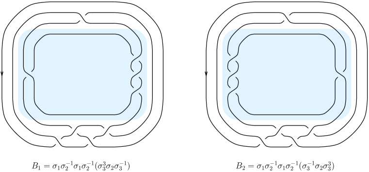
Figure 4. Two braids $B_{1},B_{2}$ whose closure is the knot $m(7_{6})$. To see that they produce the same knot, note that their closures are related by a negative flype (the shaded regions).

As one example, consider the transverse knots given by the closures of the braids $B_{1},B_{2}$ given in Figure 4, both of which are of topological type $m(7_{6})$ and have self-linking number $-1$. For each braid, one can count the number of augmentations of $(\widehat{\mathcal{A}},\widehat{\partial})$ to $\mathbb{Z}_{3}$; this augmentation number is a transverse invariant. A computer calculation shows that the augmentation number is $0$ for $B_{1}$ and $5$ for $B_{2}$. It follows that the transverse knots corresponding to $B_{1}$ and $B_{2}$ are not transversely isotopic.

One can heuristically gauge the relative effectiveness of various transverse invariants by using the Legendrian knot atlas [CN13], which provides a conjecturally complete list of all Legendrian knots representing topological knots of arc index $\leq 9$. The atlas proposes $13$ knots with arc index $\leq 9$ that have at least two transverse representatives with the same self-linking number. Of these $13$:

• $6$ ($m(7_{2})$, $m(10_{132})$, $m(10_{140})$, $m(10_{145})$, $m(10_{161})$, $12n_{591}$) have transverse representatives that can be distinguished by both the HFK invariant and by transverse homology;

• $4$ ($m(7_{6})$, $9_{44}$, $9_{48}$, $10_{136}$) can be distinguished by transverse homology but not the HFK invariant;

• $3$ ($m(9_{45})$, $10_{128}$, $10_{160}$) cannot yet be distinguished by either HFK or transverse homology.

Of these last $3$, preliminary joint work with Dylan Thurston suggests that $m(9_{45})$ and $10_{128}$ can be distinguished by naturality in conjunction with the HFK invariant, but the third cannot. It is conceivable that some or all of these last $3$ can be distinguished by transverse homology, but they are related by an operation known as “transverse mirroring” that is relatively difficult to detect by transverse homology.

It appears that the two known effective transverse invariants, the transverse HFK invariant and transverse homology, are functionally independent, but it would be very interesting to know if there is some connection between them.

Appendix: Conventions and the Fully Noncommutative DGA

In the literature on knot contact homology, a number of mutually inconsistent conventions are used. The conventions that we have adopted in this article are unfortunately different again from the existing ones, but we would like to advocate these new conventions as combining the best qualities of previous ones while avoiding some disadvantages that have become apparent in the interim.

First we describe how to extend the definition of knot contact homology from Section 3 in two directions: first, by allowing for multi-component links, and second, by extending to the fully noncommutative DGA (see Remark 2.2), in which homology classes do not commute with Reeb chords. The result is a “stronger” formulation of (combinatorial) knot contact homology than usually appears in the literature. After this, we will discuss how this definition compares to previous conventions.

If $K$ is a link given by the closure of a braid $B\in B_{n}$, we can define a slightly more complicated version of the braid homomorphism $\phi_{B}$ from Section 3 as follows. Let $\tilde{\mathcal{A}}_{n}$ denote the tensor algebra over $\mathbb{Z}$ freely generated by $a_{ij}$, $1\leq i\neq j\leq n$, and by $\tilde{\mu}_{i}^{\pm 1}$, $1\leq i\leq n$. (Here the $\tilde{\mu}_{i}$’s do not commute with the $a_{ij}$’s, or indeed with each other, and the only nontrivial relations are $\tilde{\mu}_{i}\cdot\tilde{\mu}_{i}^{-1}=\tilde{\mu}_{i}^{-1}\cdot\tilde{\mu}_{i}=1$.) For $1\leq k\leq n-1$, define $\phi_{\sigma_{k}}:\thinspace\tilde{\mathcal{A}}_{n}\to\tilde{\mathcal{A}}_{n}$ by:

$$\phi_{\sigma_{k}}:\thinspace\begin{cases}a_{ij}\mapsto a_{ij},&i,j\neq k,k+1\\ a_{k+1,i}\mapsto a_{ki},&i\neq k,k+1\\ a_{i,k+1}\mapsto a_{ik},&i\neq k,k+1\\ a_{k,k+1}\mapsto-a_{k+1,k}&\\ a_{k+1,k}\mapsto-\tilde{\mu}_{k}a_{k,k+1}\tilde{\mu}_{k+1}^{-1}&\\ a_{ki}\mapsto a_{k+1,i}-a_{k+1,k}a_{ki},&i\neq k,k+1\\ a_{ik}\mapsto a_{i,k+1}-a_{ik}a_{k,k+1},&i<k\\ a_{ik}\mapsto a_{i,k+1}-a_{ik}\tilde{\mu}_{k}a_{k,k+1}\tilde{\mu}_{k+1}^{-1},&i>k+1\\ \tilde{\mu}_{i}^{\pm 1}\mapsto\tilde{\mu}_{i}^{\pm 1},&i\neq k,k+1\\ \tilde{\mu}_{k}^{\pm 1}\mapsto\tilde{\mu}_{k+1}^{\pm 1}&\\ \tilde{\mu}_{k+1}^{\pm 1}\mapsto\tilde{\mu}_{k}^{\pm 1}.&\end{cases}$$

This extends to a group homomorphism $\phi:\thinspace B_{n}\to\operatorname{Aut}\tilde{\mathcal{A}}_{n}$ and thus defines a map $\phi_{B}\in\operatorname{Aut}\tilde{\mathcal{A}}_{n}$.

Suppose that $K$ has $r$ components, and number the components of $K$ $1,\ldots,r$. For $i=1,\ldots,n$, define $\alpha(i)\in\{1,\ldots,r\}$ to be the number of the component containing strand $i$ of the braid $B$ whose closure is $K$. If we now define $\mathcal{A}_{n}$ to be the tensor algebra over $\mathbb{Z}$ freely generated by the $a_{ij}$’s and by variables $\mu_{1}^{\pm 1},\ldots,\mu_{r}^{\pm 1}$, then it is easy to check that $\phi_{B}$ descends to an algebra automorphism of $\mathcal{A}_{n}$ by setting $\tilde{\mu}_{i}=\mu_{\alpha(i)}$ for all $1\leq i\leq n$. We can define $\Phi^{L}_{B},\Phi^{R}_{B}\in\operatorname{Mat}_{n\times n}(\mathcal{A}_{n})$ as in Definition 3.9, with the important caveat that the extra strand $\ast$ is treated as strand $0$ rather than strand $n+1$; for multi-component links, this makes a difference because of the form of the definition of $\phi_{\sigma_{k}}$ above.

Define $\mathcal{A}$ to be the tensor algebra over $\mathbb{Z}[U^{\pm 1}]$ freely generated by $\mu_{1}^{\pm 1},\ldots,\mu_{r}^{\pm 1}$ along with the generators $a_{ij},b_{ij},c_{ij},d_{ij},e_{ij},f_{ij}$ as in Definition 3.11. Assemble $n\times n$ matrices $\mathbf{A},\hat{\mathbf{A}},\mathbf{B},\hat{\mathbf{B}},\mathbf{C},\mathbf{D},\mathbf{E},\mathbf{F}$, where $\mathbf{C},\mathbf{D},\mathbf{E},\mathbf{F}$ are as in Definition 3.11, while

$$\mathbf{A}_{ij} =\begin{cases}a_{ij}&i<j\\ -a_{ij}\mu_{\alpha(j)}&i>j\\ 1-\mu_{\alpha(i)}&i=j\\ \end{cases} \mathbf{B}_{ij} =\begin{cases}b_{ij}&i<j\\ -b_{ij}\mu_{\alpha(j)}&i>j\\ 0&i=j\\ \end{cases}$$

$$(\hat{\mathbf{A}})_{ij} =\begin{cases}Ua_{ij}&i<j\\ -a_{ij}\mu_{\alpha(j)}&i>j\\ U-\mu_{\alpha(i)}&i=j\\ \end{cases} (\hat{\mathbf{B}})_{ij} =\begin{cases}Ub_{ij}&i<j\\ -b_{ij}\mu_{\alpha(j)}&i>j\\ 0&i=j.\\ \end{cases}$$

Also define a matrix $\mathbf{\Lambda}$ as follows: choose one strand of $B$ belonging to each component of the closure $K$, and call the resulting $r$ strands leading; then define

$$(\mathbf{\Lambda})_{ij}=\begin{cases}\lambda_{\alpha(i)}\mu_{\alpha(i)}^{w(\alpha(i))}U^{-(w(\alpha(i))-n(\alpha(i))+1)/2}&i=j\text{ and strand $i$ leading}\\ 1&i=j\text{ and strand $i$ not leading}\\ 0&i\neq j,\end{cases}$$

where $n(\alpha)$ is the number of strands belonging to component $\alpha$ and $w(\alpha)$ is the writhe of component $\alpha$ viewed as an $n(\alpha)$-strand braid (with the other components deleted).

With this notation, one can now define the differential $\partial$ on $\mathcal{A}$ exactly as in Definition 3.11. The resulting DGA has the same properties as in Theorem 3.15: $\partial^{2}=0$ and $(\mathcal{A},\partial)$ is an isotopy invariant of the link $K$ viewed as an oriented link with numbered components, up to stable tame isomorphisms that act as the identity on $U$ and on each of $\lambda_{1},\ldots,\lambda_{r},\mu_{1},\ldots,\mu_{r}$.

Note that the definition of the DGA given above is for the topological knot/link invariant as discussed in Sections 2 and 3. This corresponds to “infinity transverse homology” from [Ng11] (also mentioned in [EENS13a]). There is an analogous definition of transverse homology as in Section 6 or [EENS13a, Ng11] but we omit its definition here.

We now compare our definition to the two previous conventions for the knot DGA: the convention from [EENS13a, EENS13b] and the convention from [Ng11, Ng08]. Note that all versions of the DGA from these references first quotient so that homology classes $\lambda_{1},\ldots,\lambda_{r},\mu_{1},\ldots,\mu_{r}$ commute with all Reeb chords. Also, the versions from [EENS13a] and [Ng11] involve an additional variable $V$, but we set $V=1$ for this discussion; as explained in [Ng11, §4], this does not lose any information. Finally, the conventions from [EENS13b] and [Ng08] agree with the conventions from [EENS13a] and [Ng11], respectively, after setting $U=V=1$.

We claim that we can then obtain the knot DGAs in the conventions of [EENS13a] and [Ng11] from the knot DGA presented in this article, up to isomorphism, as follows:

• for [EENS13a], replace $\lambda_{\alpha}\mapsto-\lambda_{\alpha}$ and $\mu_{\alpha}\mapsto-\mu_{\alpha}$ for each component $\alpha$;

• for [Ng11], which only considers the single-component case, keep $\lambda$ as is, and replace $\mu\mapsto-\mu^{-1}$.

We check the claim for the convention of [EENS13a]; the claim for [Ng11] then follows from [Ng11, §3.4]. Note that negating each $\lambda_{\alpha}$ and $\mu_{\alpha}$ causes our definitions to line up precisely with the definitions from [EENS13a], except for $\mathbf{\Lambda}$ (denoted in [EENS13a] by -$\boldsymbol{\lambda}$), which differs by the presence or absence of a power of $U$, along with some signs. But the power of $U$ is merely a notational/framing issue (cf. [Ng11]), while the sign discrepancy disappears because it can be checked that the products of the diagonal entries of $\mathbf{\Lambda}$ and $-\boldsymbol{\lambda}$ corresponding to any particular link component are exactly equal including sign, whence the DGAs given by the two conventions are isomorphic by the argument of [Ng11, Proposition 3.1].

Remark 6.10.

Except for the $\mu\mapsto\mu^{-1}$ issue, all differences between conventions consist just of negating some subset of $\{\lambda,\mu\}$. This is explained by the fact that the signs in the differential in Legendrian contact homology depend on a choice of spin structure on the Legendrian submanifold $\Lambda$; see [EES05] for full discussion. In our setting, if $K$ is a knot, $\Lambda_{K}\cong T^{2}$ has four spin structures, and changing from one spin structure to another sends $\lambda\mapsto\pm\lambda$ and $\mu\mapsto\pm\mu$. Thus the different choices of signs arise from different choices of spin structure on $\Lambda_{K}$.

A summary of the relations between conventions in different articles is as follows:

We close by noting that our current choice of conventions allows for some cleaner results than the conventions from [EENS13a] or [Ng11]. In particular, our signs are more natural than the signs from either [EENS13a] or [Ng11] when we consider the relation to representations of the knot group as in Section 5. For instance, our two-variable augmentation polynomials are divisible by $(\lambda-1)(\mu-1)$ as opposed to $(\lambda+1)(\mu+1)$ in [EENS13a] or $(\lambda-1)(\mu+1)$ in [Ng11, Ng08], and $A_{K}(\lambda,\mu)$ divides $\operatorname{Aug}_{K}(\lambda,\mu^{2})$ in our convention rather than $\operatorname{Aug}_{K}(-\lambda,-\mu^{2})$ or $\operatorname{Aug}_{K}(\lambda,-\mu^{2})$ in the other two.

There is another technical reason for preferring our signs or those from [EENS13a] to the ones from [Ng11], or more precisely to the extrapolation of [Ng11] to the link case. In either of the first two cases but not the third, we have the following statement, which we leave as an exercise.

Proposition 6.11.

Let $K$ be a link given by the closure of braid $B$, and let $K^{\prime}\subset K$ be a sublink given by the closure of a subbraid $B^{\prime}\subset B$ obtained by erasing some strands of $B$. Then the DGA for $K^{\prime}$ is a quotient of the DGA for $K$, given by setting all Reeb chords $a_{ij},b_{ij},$ etc. to $0$ unless strands $i$ and $j$ both belong to $B^{\prime}$.

This result is used in [AENV] and is a special case of a general result relating the Legendrian contact homology of a multi-component Legendrian to the LCH of some subset of components.

References

- [Abo12] Mohammed Abouzaid. Framed bordism and Lagrangian embeddings of exotic spheres. Ann. of Math. (2), 175(1):71–185, 2012. arXiv:0812.4781.
- [AENV] Mina Aganagic, Tobias Ekholm, Lenhard Ng, and Cumrun Vafa. Topological strings, -model, and knot contact homology. arXiv:1304.5778.
- [AS06] Alberto Abbondandolo and Matthias Schwarz. On the Floer homology of cotangent bundles. Comm. Pure Appl. Math., 59(2):254–316, 2006. arXiv:math/0408280.
- [AS10] Alberto Abbondandolo and Matthias Schwarz. Floer homology of cotangent bundles and the loop product. Geom. Topol., 14(3):1569–1722, 2010. arXiv:0810.1995.
- [AV] Mina Aganagic and Cumrun Vafa. Large duality, mirror symmetry, and a Q-deformed A-polynomial. arXiv:1204.4709.
- [Ben83] Daniel Bennequin. Entrelacements et équations de Pfaff. In Third Schnepfenried geometry conference, Vol. 1 (Schnepfenried, 1982), volume 107 of Astérisque, pages 87–161. Soc. Math. France, Paris, 1983.
- [Che02] Yuri Chekanov. Differential algebra of Legendrian links. Invent. Math., 150(3):441–483, 2002.
- [CL09] Kai Cieliebak and Janko Latschev. The role of string topology in symplectic field theory. In New perspectives and challenges in symplectic field theory, volume 49 of CRM Proc. Lecture Notes, pages 113–146. Amer. Math. Soc., Providence, RI, 2009. arXiv:0706.3284.
- [CN13] Wutichai Chongchitmate and Lenhard Ng. An atlas of Legendrian knots. Exp. Math., 22(1):26–37, 2013. arXiv:1010.3997.
- [DG04] Nathan M. Dunfield and Stavros Garoufalidis. Non-triviality of the -polynomial for knots in . Algebr. Geom. Topol., 4:1145–1153 (electronic), 2004. arXiv:math/0405353.
- [EE05] Tobias Ekholm and John B. Etnyre. Invariants of knots, embeddings and immersions via contact geometry. In Geometry and topology of manifolds, volume 47 of Fields Inst. Commun., pages 77–96. Amer. Math. Soc., Providence, RI, 2005. arXiv:math/0412517.
- [EENS13a] Tobias Ekholm, John Etnyre, Lenhard Ng, and Michael Sullivan. Filtrations on the knot contact homology of transverse knots. Math. Ann., 355(4):1561–1591, 2013. arXiv:1010.0450.
- [EENS13b] Tobias Ekholm, John B. Etnyre, Lenhard Ng, and Michael G. Sullivan. Knot contact homology. Geom. Topol., 17(2):975–1112, 2013. arXiv:1109.1542.
- [EES05] Tobias Ekholm, John Etnyre, and Michael Sullivan. Orientations in Legendrian contact homology and exact Lagrangian immersions. Internat. J. Math., 16(5):453–532, 2005. arXiv:math/0408411.
- [EES07] Tobias Ekholm, John Etnyre, and Michael Sullivan. Legendrian contact homology in . Trans. Amer. Math. Soc., 359(7):3301–3335 (electronic), 2007. arXiv:math/0505451.
- [EGH00] Y. Eliashberg, A. Givental, and H. Hofer. Introduction to symplectic field theory. Geom. Funct. Anal., (Special Volume, Part II):560–673, 2000. GAFA 2000 (Tel Aviv, 1999). arXiv:math/0010059.
- [Ekh07] Tobias Ekholm. Morse flow trees and Legendrian contact homology in 1-jet spaces. Geom. Topol., 11:1083–1224, 2007. arXiv:math/0509386.
- [Eli98] Yakov Eliashberg. Invariants in contact topology. In Proceedings of the International Congress of Mathematicians, Vol. II (Berlin, 1998), number Extra Vol. II, pages 327–338 (electronic), 1998.
- [ENS02] John B. Etnyre, Lenhard L. Ng, and Joshua M. Sabloff. Invariants of Legendrian knots and coherent orientations. J. Symplectic Geom., 1(2):321–367, 2002. arXiv:math/0101145.
- [FGS13] Hiroyuki Fuji, Sergei Gukov, and Piotr Sułkowski. Super--polynomial for knots and BPS states. Nuclear Phys. B, 867(2):506–546, 2013. arXiv:1205.1515.
- [Gar] Stavros Garoufalidis. The colored HOMFLY polynomial is -holonomic. arXiv:1211.6388.
- [Gar04] Stavros Garoufalidis. On the characteristic and deformation varieties of a knot. In Proceedings of the Casson Fest, volume 7 of Geom. Topol. Monogr., pages 291–309 (electronic). Geom. Topol. Publ., Coventry, 2004. arXiv:math/0306230.
- [GSV05] Sergei Gukov, Albert Schwarz, and Cumrun Vafa. Khovanov-Rozansky homology and topological strings. Lett. Math. Phys., 74(1):53–74, 2005. arXiv:hep-th/0412243.
- [GV01] Rajesh Gopakumar and Cumrun Vafa. On the gauge theory/geometry correspondence. In Winter School on Mirror Symmetry, Vector Bundles and Lagrangian Submanifolds (Cambridge, MA, 1999), volume 23 of AMS/IP Stud. Adv. Math., pages 45–63. Amer. Math. Soc., Providence, RI, 2001. arXiv:hep-th/9811131.
- [KM04] P. B. Kronheimer and T. S. Mrowka. Dehn surgery, the fundamental group and SU. Math. Res. Lett., 11(5-6):741–754, 2004. arXiv:math/0312322.
- [Kna] Adam Knapp. Symplectic structures on the cotangent bundles of open -manifolds. arXiv:1209.3045.
- [KR08] Mikhail Khovanov and Lev Rozansky. Matrix factorizations and link homology. II. Geom. Topol., 12(3):1387–1425, 2008. arXiv:math/0505056.
- [LOSS09] Paolo Lisca, Peter Ozsváth, András I. Stipsicz, and Zoltán Szabó. Heegaard Floer invariants of Legendrian knots in contact three-manifolds. J. Eur. Math. Soc. (JEMS), 11(6):1307–1363, 2009. arXiv:0802.0628.
- [Mag80] Wilhelm Magnus. Rings of Fricke characters and automorphism groups of free groups. Math. Z., 170(1):91–103, 1980.
- [Ng05a] Lenhard Ng. Knot and braid invariants from contact homology. I. Geom. Topol., 9:247–297 (electronic), 2005. arXiv:math/0302099.
- [Ng05b] Lenhard Ng. Knot and braid invariants from contact homology. II. Geom. Topol., 9:1603–1637 (electronic), 2005. With an appendix by the author and Siddhartha Gadgil. arXiv:math/0303343.
- [Ng06] Lenhard Ng. Conormal bundles, contact homology and knot invariants. In The interaction of finite-type and Gromov-Witten invariants (BIRS 2003), volume 8 of Geom. Topol. Monogr., pages 129–144. Geom. Topol. Publ., Coventry, 2006. arXiv:math/0412330.
- [Ng08] Lenhard Ng. Framed knot contact homology. Duke Math. J., 141(2):365–406, 2008. arXiv:math/0407071.
- [Ng11] Lenhard Ng. Combinatorial knot contact homology and transverse knots. Adv. Math., 227(6):2189–2219, 2011. arXiv:1010.0451.
- [NOT08] Lenhard Ng, Peter Ozsváth, and Dylan Thurston. Transverse knots distinguished by knot Floer homology. J. Symplectic Geom., 6(4):461–490, 2008. arXiv:math/0703446.
- [OS03] S. Yu. Orevkov and V. V. Shevchishin. Markov theorem for transversal links. J. Knot Theory Ramifications, 12(7):905–913, 2003. arXiv:math/0112207.
- [OST08] Peter Ozsváth, Zoltán Szabó, and Dylan Thurston. Legendrian knots, transverse knots and combinatorial Floer homology. Geom. Topol., 12(2):941–980, 2008. arXiv:math/0611841.
- [OV00] Hirosi Ooguri and Cumrun Vafa. Knot invariants and topological strings. Nuclear Phys. B, 577(3):419–438, 2000. arXiv:hep-th/9912123.
- [Per10] Tim Perutz. The symplectic topology of cotangent bundles. Eur. Math. Soc. Newsl., (75):30–33, 2010.
- [SW06] D. A. Salamon and J. Weber. Floer homology and the heat flow. Geom. Funct. Anal., 16(5):1050–1138, 2006. arXiv:math/0304383.
- [Vit] Claude Viterbo. Functors and computations in Floer homology with applications. II. Preprint, 1996. Available at http://www.math.polytechnique.fr/ cmat/viterbo/Prepublications.html.
- [Wri] Nancy C. Wrinkle. The Markov Theorem for transverse knots. arXiv:math/0202055.