Disordered bosons in one dimension: from weak to strong randomness criticality

Abstract

We investigate the superfluid-insulator quantum phase transition of one-dimensional bosons with off-diagonal disorder by means of large-scale Monte-Carlo simulations. For weak disorder, we find the transition to be in the same universality class as the superfluid-Mott insulator transition of the clean system. The nature of the transition changes for stronger disorder. Beyond a critical disorder strength, we find nonuniversal, disorder-dependent critical behavior. We compare our results to recent perturbative and strong-disorder renormalization group predictions. We also discuss experimental implications as well as extensions of our results to other systems.

Bosonic many-particle systems can undergo quantum phase transitions between superfluid and localized ground states due to interactions and lattice effects. These superfluid-insulator transitions occur in a wide variety of experimental systems ranging from helium in porous media, Josephson junction arrays, and granular superconductors to ultracold atomic gases Crooker et al. (1983); Chan et al. (1988); Haviland et al. (1989); Hebard and Paalanen (1990); Bezryadin et al. (2000); Greiner et al. (2002); Damski et al. (2003); Fallani et al. (2007). In many of these applications, the bosons are subject to quenched disorder or randomness. Understanding the effects of disorder on the superfluid-insulator transition and on the resulting insulating phases is thus a prime question.

The case of one space dimension is especially interesting because the superfluid phase is rather subtle and displays quasi-long-range order instead of true long-range order. Moreover, the Anderson localization scenario for non-interacting bosons suggests that disorder becomes more important with decreasing dimensionality.

Giarmarchi and Schulz Giamarchi and Schulz (1987); *GiamarchiSchulz88 studied the influence of weak disorder on the interacting superfluid by means of a perturbative renormalization group analysis. They found the superfluid-insulator transition to be of Kosterlitz-Thouless (KT) type Kosterlitz and Thouless (1973), with universal critical exponents and a universal value of the Luttinger parameter $g=\pi\sqrt{\rho_{s}\kappa}$ at criticality ($\rho_{s}$ denotes the superfluid stiffness and $\kappa$ the compressibility). This analysis was recently extended to second order in the disorder strength, with unchanged conclusion Ristivojevic et al. (2012).

A different scenario emerges, however, from the real-space strong-disorder renormalization group approach. In a series of papers Altman et al. (2004); *AKPR08; *AKPR10, Altman et al. studied one-dimensional interacting lattice bosons in various types of disorder. In all cases, they found that the superfluid-insulator transition is characterized by KT-like scaling of lengths and times, but it occurs at a nonuniversal, disorder-dependent value of the Luttinger parameter. The transition is thus in a different universality class than the weak-disorder transition Giamarchi and Schulz (1987, 1988). However, Monte-Carlo simulations Balabanyan et al. (2005) did not find any evidence in favor of the strong-disorder critical point.

In view of these seemingly incompatible results, it is important to determine whether or not both types of superfluid-insulator critical points indeed exist in systems of interacting disordered bosons in one dimension. Moreover, it is important to study whether they can be reached for realistic disorder strengths.

In this Letter, we employ large-scale Monte-Carlo simulations to address these questions. We focus on the case of off-diagonal disorder at large commensurate filling; other types of disorder will be discussed in the conclusions. Our results can be summarized as follows (see Fig. 1).

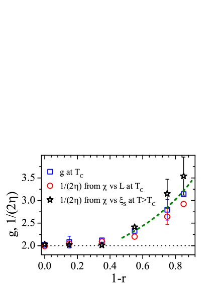
Figure 1: (Color online) Critical Luttinger parameter $g$ and exponent $\eta$ [plotted as $1/(2\eta)$] of the superfluid-insulator transition as functions of the disorder strength $1-r$. The critical behavior appears universal for weak disorder while it becomes disorder-dependent for strong disorder. The lines are guides to the eye only.

For weak disorder, we find a KT critical point in the universality class of the clean (1+1) dimensional XY model, with universal exponents and a universal value of the Luttinger parameter at the transition. This agrees with the predictions of the perturbative renormalization group. If the disorder strength is increased beyond a threshold value, the nature of the transition changes. While the scaling of length and time scales remains KT-like, the critical exponents and the Luttinger parameter become non-universal, in agreement with the strong-disorder scenario Altman et al. (2004); *AKPR08; *AKPR10. In the remainder of this Letter, we explain how these results were obtained, we discuss their generality as well as implications for experiment.

The starting point is the disordered one-dimensional quantum rotor Hamiltonian

$$H=-\sum_{j}J_{j}\cos(\hat{\phi}_{j+1}-\hat{\phi}_{j})+\frac{1}{2}\sum_{j}U_{j}(\hat{n}_{j}-\bar{n}_{j})^{2}$$ (1)

which represents, e.g., a chain of superfluid grains with Josephson couplings $J_{j}$, charging energies $U_{j}$ and offset charges $\bar{n}_{j}$. $\hat{n}_{j}$ is the charge on grain $j$ and $\hat{\phi}_{j}$ is the phase of the superfluid order parameter. This model has a superfluid ground state if the Josephson couplings dominate. With increasing charging energies it undergoes a quantum phase transition to an insulating ground state. In addition to Josephson junction arrays, the Hamiltonian (1) describes a wide variety of other systems that undergo superfluid-insulator transitions.

Within the strong-disorder approach Altman et al. (2004); *AKPR08; *AKPR10, the type of insulator depends on the symmetry properties of the offset charge distribution. In contrast, these details were found unimportant at the critical point. In the following, we therefore focus on purely off-diagonal disorder, $\bar{n}_{j}=0$. In this case, the Hamiltonian (1) can be mapped onto a classical $(1+1)$-dimensional XY model Wallin et al. (1994)

$$H_{\rm cl}=-\sum_{j,\tau}\left[J^{s}_{j}\cos(\phi_{j+1,\tau}-\phi_{j,\tau})+J^{t}_{j}\cos(\phi_{j,\tau+1}-\phi_{j,\tau})\right]$$ (2)

where $j$ and $\tau$ index the lattice sites in the space and time-like directions, respectively. The coupling constants $J^{s}_{j}/T$ and $J^{t}_{j}/T$ are determined by the parameters of the original Hamiltonian (1) with $T$ being an effective “classical” temperature, not equal to the real physical temperature which is zero. In the following, we fix $J^{s}_{j}$ and $J^{t}_{j}$ and drive the XY model (2) through the transition by tuning $T$. The interactions $J^{s}_{j}$ and/or $J^{t}_{j}$ are independent random variables drawn from probability distributions $P^{s}(J^{s})$ and $P^{t}(J^{t})$. They depend on the space coordinate $j$ only; this means the disorder is columnar (perfectly correlated in time direction).

To determine the critical behavior of the classical XY model (2), we performed large-scale Monte-Carlo simulations using the efficient Wolff cluster algorithm Wolff (1989). We studied square lattices with linear sizes up to $L=3200$ and averaged the results over large numbers (200 to 3000, depending on $L$) of disorder realizations. Each sample was equilibrated using 200 to 400 Monte-Carlo sweeps, i.e., total spin flips per site. (The actual equilibration times both above and at the critical temperature $T_{c}$ did not exceed about 20 sweeps.) During the measurement period of 5000 to 30000 sweeps, we calculated observables such as specific heat, magnetization, susceptibility, spin-wave stiffness as well as correlation functions. In most simulations, we employed a uniform $J^{s}_{j}=1$ and drew the $J^{t}_{j}$ from a binary probability distribution

$$P^{t}(J^{t})=c\delta(J^{t}-r)+(1-c)\delta(J^{t}-1)~{}.$$ (3)

Here, $c$ is the concentration of weak bonds which we fixed at $c=0.8$. The disorder strength was tuned by changing the value $r$ of the weak bonds. In addition to the clean case $r=1$ (which corresponds to the pure superfluid-Mott insulator transition), we used $r=0.85,0.65,0.45,0.25$, and 0.15. We also carried out test calculations with random $J^{s}$. All simulations were performed on the Pegasus Cluster at Missouri S&T, using about 400,000 CPU hours

We now turn to the results. To find $T_{c}$ for each disorder strength $r$, we analyzed the behavior of the correlation length $\xi_{s}$ (in the space-like direction indexed by $j$). It is calculated, as usual, from the second moment of the disorder-averaged correlation function. In the high-temperature phase but close to the transition, $\xi_{s}$ is expected to follow the form

$$\xi_{s}=A\exp\left[B(T-T_{c})^{-1/2}\right]$$ (4)

both in the clean KT universality class Kosterlitz and Thouless (1973) and in the strong-disorder scenario Altman et al. (2004); *AKPR08; *AKPR10. $A$ and $B$ are non-universal constants. For all disorder strength, our data follow this prediction with high accuracy, see Fig. 2 for an example.

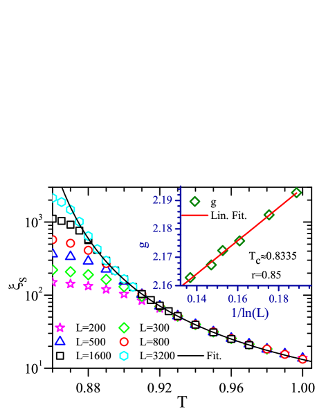
Figure 2: (Color online) Spatial correlation length $\xi_{s}$ vs. temperature $T$ for disorder strength $r=0.85$ and system sizes $L=200$ to 3200. The solid line is a fit to the KT form (4). Inset: Luttinger parameter $g$ at $T_{c}$ vs. system size $L$.

We extract $T_{c}$ from fits of the data to (4) restricted to $\xi_{s}>10$ to be in the critical region but $\xi_{s}<L/10$ to avoid finite-size effects. In the clean case ($r=1$), we obtain $T_{c}=0.8924$ in excellent agreement with high-precision values in the literature Hasenbusch (2005) .

In addition to the correlation length $\xi_{s}$ in the space-like direction, we also studied the correlation length $\xi_{t}$ in the time-like direction. We found $\xi_{t}\propto\xi_{s}$ for all disorder strengths which implies a dynamical exponent of $z=1$.

The order parameter susceptibility $\chi$ can be analyzed analogously. In the high-temperature phase close to the transition, it is predicted to behave as

$$\chi\propto\xi_{s}^{2-\eta}\propto\exp\left[D(T-T_{c})^{-1/2}\right]~{}.$$ (5)

Here, $\eta$ is the correlation function critical exponent and $D=(2-\eta)B$. Figure 3 shows that the data for all disorder strengths $r$ follow this prediction with high accuracy.

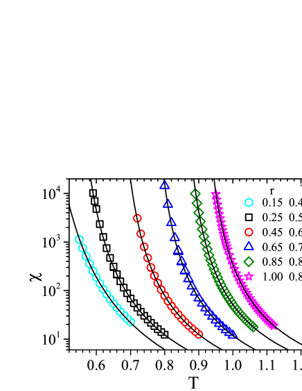
Figure 3: (Color online) Susceptibility $\chi$ vs. temperature $T$ for several disorder strengths. The maximum system sizes are at least $L=1500$. The solid lines are fits to the KT form (5). The resulting estimates of $T_{c}$ are listed in the legend.

The critical temperatures extracted from the corresponding fits are listed in the legend of the figure. Their values have small statistical errors ranging from about $3\times 10^{-4}$ for the weak disorder cases to $2\times 10^{-3}$ for strong disorder. The systematic errors due to corrections to the leading scaling form (5) are somewhat larger. We estimate them from the robustness of the fit against changing the fit interval. This yields systematic errors ranging from about $5\times 10^{-3}$ for weak disorder to $2\times 10^{-2}$ for strong disorder. Within these errors the critical temperatures extracted from $\chi$ agree well with those from the correlation lengths.

Equation (5) suggests a direct way to measure the exponent $\eta$: if one plots $\ln(\chi/\xi_{s}^{2})$ vs. $\ln(\xi_{s})$, the data should be on a straight line with slope $-\eta$. Figure 4 presents this analysis for different disorder strengths.

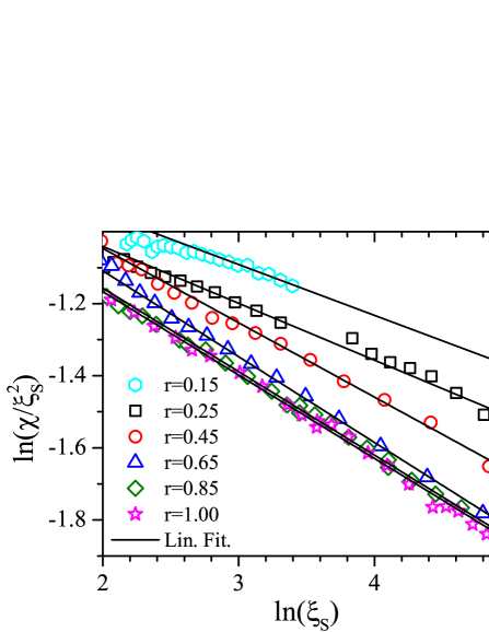
Figure 4: (Color online) $\ln(\chi/\xi^{2}_{s})$ vs. $\ln(\xi_{s})$ for several disorder strengths and maximum system size $L\geq 1500$ ($L=500$ for $r=0.15$). The solid lines are linear fits; their slopes give $-\eta$.

In the clean case, $r=1$, we find $\eta=0.243$ in good agreement with the exact value 1/4 Kosterlitz and Thouless (1973). The weak-disorder curves ($r=0.85$ and 0.65) are parallel to the clean one within their statistical errors. Fits in the range $20<\xi_{s}<L/10$ give exponents $\eta$ close to $1/4$. In contrast, the strong-disorder curves ($r=0.45$, 0.25, 0.15) are less steep, resulting in smaller $\eta$. They are also noisier which leads to larger error bars. All $\eta$ values are shown in Fig. 1. They provide evidence for universal critical behavior (in the clean 2D XY universality class) for weak disorder but nonuniversal behavior for strong disorder.

In addition to simulations in the high-temperature phase, we also studied the finite-size scaling properties of observables right at the critical temperature $T_{c}$. Let us first consider the Luttinger parameter $g=\pi\sqrt{\rho_{s}\kappa}$. Under the quantum-to-classical mapping Wallin et al. (1994), the compressibility $\kappa$ of the quantum rotor Hamiltonian (1) maps onto the spin-wave stiffness $\rho_{t}$ in the time-like direction of the classical XY model (2). In our simulations, the Luttinger parameter is thus given by

$$g=(\pi/T)\sqrt{\rho_{s}\rho_{t}}~{}.$$ (6)

The stiffnesses $\rho_{s}$ and $\rho_{t}$ are not calculated by actually applying twisted boundary conditions during the simulation but by using the relation given by Teitel and Jayaprakash Teitel and Jayaprakash (1983) (for a derivation see, e.g., Ref. Hrahsheh et al. (2011)).

Within KT theory, the Luttinger parameter close to the transition behaves as $g(T)=g(T_{c})+a(T_{c}-T)^{1/2}$ where $a$ is a constant and $T\leq T_{c}$. Together with (4), this suggests the leading finite-size corrections to $g$ at $T_{c}$ to take the form

$$g(T_{c},L)=g(T_{c},\infty)+b/\ln(L)$$ (7)

where $b$ is another constant. Calculating the Luttinger parameter at $T_{c}$ for different system sizes and extrapolating using (7) yields the infinite-system value $g(T_{c},\infty)$ . We performed this analysis for all disorder strengths $r$ and found that the $g$ vs. $1/\ln(L)$ data indeed fall onto straight lines (the inset of Fig. 2 shows an example). The resulting extrapolated values are displayed in Fig. 1. For weak disorder ($r=0.85$ and 0.65), the Luttinger parameters at $T_{c}$ agree with the clean value, $g=2$, within their error bars (which are combinations of the statistical Monte-Carlo error and the uncertainty in $T_{c}$). For stronger disorder ($r=0.45$, 0.25, 0.15), $g(T_{c},\infty)$ takes larger, disorder-dependent values.

Finally, we turn to the finite-size behavior of the susceptibility at $T_{c}$. According to finite-size scaling, the leading size-dependence should be of the form

$$\chi(T_{c},L)\sim L^{2-\eta}$$ (8)

which provides another way to measure $\eta$. Figure 5 shows plots of $\ln(\chi/L^{2})$ vs. $\ln(L)$ for all disorder strengths $r$.

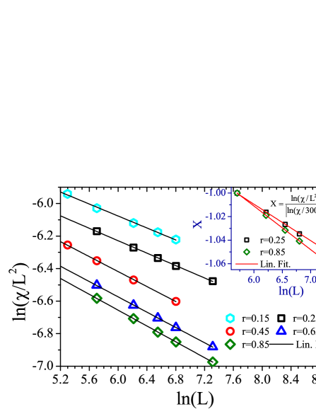
Figure 5: (Color online) Susceptibility at $T_{c}$ plotted as $\ln(\chi/L^{2}_{s})$ vs. $\ln(L)$ for several disorder strengths. The solid lines are linear fits; their slopes give $-\eta$ (values are shown in Fig. 1) . The inset demonstrates the change of slope with increasing $r$.

For weak disorder ($r=0.85$ and 0.65), the resulting values of the exponent $\eta$ are again close to the clean value $1/4$. For larger disorder ($r=0.45$, 0.25, and 0.15), we find disorder-dependent values that roughly agree with those extracted in the high-temperature phase (Fig. 4).

In summary, we used large-scale Monte-Carlo simulations to investigate the superfluid-insulator quantum phase transition of one-dimensional bosons with off-diagonal disorder. For weak disorder, our data provide evidence for a KT critical point in the universality class of the clean (1+1) dimensional classical XY model, with universal critical exponents $\eta=1/4$ and $z=1$ as well as a universal value $g=2$ of the critical Luttinger parameter. These results agree with the Harris criterion Harris (1974) which predicts weak disorder to be an irrelevant perturbation at the clean KT transition. For stronger disorder, the universality class of the transition changes. It is still of KT-type [$\xi_{s}$ and $\chi$ follow (4) and (5)] but the critical exponent $\eta$ and the critical Luttinger parameter become disorder-dependent (non-universal) . This agrees with the strong-disorder scenario Altman et al. (2004); *AKPR08; *AKPR10.

The important question of whether the boundary between the weak and strong disorder regimes is sharp or just a crossover cannot be finally decided by means of our current numerical capabilities. The data in Fig. 1 would be compatible with both scenarios within their error bars.

Earlier Monte-Carlo simulations Balabanyan et al. (2005) did not observe the strong-disorder regime. We believe that the binary disorder used in Balabanyan et al. (2005) (equivalent to disorder in $J^{s}$ with $c=0.5$ and $r=0.33$ in our model) may not have been sufficiently strong. In particular, $c=0.5$ is much less favorable for the formation of rare regions than our $c=0.8$. To test this hypothesis, we performed a few simulation using $c=0.5$ and $r=0.33$. They resulted in critical behavior compatible with the clean 2D XY universality class, in agreement with Ref. Balabanyan et al. (2005) .

It is interesting to ask whether the different critical behaviors in the weak and strong-disorder regimes are accompanied by qualitative differences in the bulk phases. In particular, are there two different insulating phases or are the weak and strong-disorder regimes continuously connected? A detailed analysis of the insulating phase(s) will also shed light on the mechanism that destroys the superfluid stiffness above $T_{c}$. Is it due to the proliferation of single quantum phase slips as at a clean KT transition or due to the formation of phase slip “dipoles” as suggested in Ref. Altman et al. (2004); *AKPR08; *AKPR10? Simulations to address these questions are under way.

All our explicit results are for off-diagonal disorder and large commensurate filling. They do not directly apply to the generic dirty-boson problem with diagonal disorder considered in Giamarchi and Schulz (1987); *GiamarchiSchulz88 . Note, however, that the critical behavior does not depend on the disorder type within the strong-disorder scenario Altman et al. (2004); *AKPR08; *AKPR10. Simulating the generic case would require a different approach (such as the link-current formulation Wallin et al. (1994)) because the mapping onto a classical XY model is not valid for diagonal disorder.

Finally, we turn to the experimental accessibility of the weak and strong-disorder regimes. Our results show that the transition between them occurs at a moderate disorder strengths. We therefore expect both regimes to be accessible in principle in experiments on systems such as ultracold atoms or Josephson junction chains (see also Ref. Vosk and Altman (2012)).

We acknowledge discussions with Ehud Altman, David Pekker, Nikolay Prokof’ev, Gil Refael, and Zoran Ristivojevic. This work has been supported by the NSF under Grant Nos. DMR-0906566 and DMR-1205803.

References

- Crooker et al. (1983) B. C. Crooker, B. Hebral, E. N. Smith, Y. Takano, and J. D. Reppy, Phys. Rev. Lett. 51, 666 (1983).
- Chan et al. (1988) M. H. W. Chan, K. I. Blum, S. Q. Murphy, G. K. S. Wong, and J. D. Reppy, Phys. Rev. Lett. 61, 1950 (1988).
- Haviland et al. (1989) D. B. Haviland, Y. Liu, and A. M. Goldman, Phys. Rev. Lett. 62, 2180 (1989).
- Hebard and Paalanen (1990) A. F. Hebard and M. A. Paalanen, Phys. Rev. Lett. 65, 927 (1990).
- Bezryadin et al. (2000) A. Bezryadin, C. N. Lau, and M. Tinkham, Nature 404, 971 (2000).
- Greiner et al. (2002) M. Greiner, O. Mandel, T. Esslinger, T. W. Hänsch, and I. Bloch, Nature 415, 39 (2002).
- Damski et al. (2003) B. Damski, J. Zakrzewski, L. Santos, P. Zoller, and M. Lewenstein, Phys. Rev. Lett. 91, 080403 (2003).
- Fallani et al. (2007) L. Fallani, J. E. Lye, V. Guarrera, C. Fort, and M. Inguscio, Phys. Rev. Lett. 98, 130404 (2007).
- Giamarchi and Schulz (1987) T. Giamarchi and H. J. Schulz, EPL (Europhysics Letters) 3, 1287 (1987).
- Giamarchi and Schulz (1988) T. Giamarchi and H. J. Schulz, Phys. Rev. B 37, 325 (1988).
- Kosterlitz and Thouless (1973) J. M. Kosterlitz and D. J. Thouless, J. Phys. C 6, 1181 (1973).
- Ristivojevic et al. (2012) Z. Ristivojevic, A. Petković, P. Le Doussal, and T. Giamarchi, Phys. Rev. Lett. 109, 026402 (2012).
- Altman et al. (2004) E. Altman, Y. Kafri, A. Polkovnikov, and G. Refael, Phys. Rev. Lett. 93, 150402 (2004).
- Altman et al. (2008) E. Altman, Y. Kafri, A. Polkovnikov, and G. Refael, Phys. Rev. Lett. 100, 170402 (2008).
- Altman et al. (2010) E. Altman, Y. Kafri, A. Polkovnikov, and G. Refael, Phys. Rev. B 81, 174528 (2010).
- Balabanyan et al. (2005) K. G. Balabanyan, N. Prokof’ev, and B. Svistunov, Phys. Rev. Lett. 95, 055701 (2005).
- Wallin et al. (1994) M. Wallin, E. S. Sorensen, S. M. Girvin, and A. P. Young, Phys. Rev. B 49, 12115 (1994).
- Wolff (1989) U. Wolff, Phys. Rev. Lett. 62, 361 (1989).
- Hasenbusch (2005) M. Hasenbusch, J. Phys. A 38, 5869 (2005).
- Note (1) The remaining small difference can be attributed to logarithmic corrections to (4) which we did not account for.
- Teitel and Jayaprakash (1983) S. Teitel and C. Jayaprakash, Phys. Rev. B 27, 598 (1983).
- Hrahsheh et al. (2011) F. Hrahsheh, H. Barghathi, and T. Vojta, Phys. Rev. B 84, 184202 (2011).
- Note (2) The extrapolation of to is nontrivial as shows a singular temperature dependence and a jump to for . The data must be in the critical region, , which appears to be fulfilled in our case.
- Harris (1974) A. B. Harris, J. Phys. C 7, 1671 (1974).
- Note (3) Fig. 1 suggests that not just at the clean KT critical point but also at the strong disorder critical point. To the best of our knowledge, the latter has not yet been established theoretically.
- Note (4) Ref. Balabanyan et al. (2005) also studied power-law distributed interactions, but the results showed significant finite-size effects.
- Note (5) The critical value of in the perturbative theory Giamarchi and Schulz (1987) with diagonal disorder is 3/2 rather than 2.
- Vosk and Altman (2012) R. Vosk and E. Altman, Phys. Rev. B 85, 024531 (2012).